1. Introduction
The use of agricultural pesticides has the potential to result in residue detections of these products and their metabolites in water bodies which can be of concern for the environment [
1]. Models can help to predict these aquatic exposure levels, identify areas vulnerable to off-site transport, and determine the most effective mitigation measures to reduce concentrations of pesticides in non-target environments. In this context, a critical component to designing and implementing mitigation practices to aid in the reduction of pesticide concentrations in surface water is a rigorous understanding of the routes of exposure to a specific water body [
2] which can be provided through hydrologic watershed models. The principles of pesticide losses from farmland and their transport to surface water bodies are well researched and implemented into various models [
3]. The Soil and Water Assessment Tool (SWAT, [
4]) has been a leading international model for predicting the fate and transport of non-point source agrochemicals at the watershed scale. Model applications have been reported in the literature since at least 2005 and since then several studies have been published from around the world (a comprehensive overview is provided in the introduction in [
5]). In 2006 SWAT was selected from a pool of 36 models as one of three that were most appropriate for watershed-scale simulation of pesticides [
3]. However, three major challenges impede the application of SWAT for pesticide exposure assessments.
First, SWAT’s capabilities to account for spatially distributed transport processes and variability in local agricultural management practices are limited. The SWAT model typically utilizes a hydrologic response unit (HRU) approach where the watershed is divided into sub-watersheds which are further subdivided into HRUs. With the HRU approach, all areas in a sub-watershed with the same combination of soil, topography, and land use are lumped to form an HRU. The HRUs represent percentages of the sub-watershed area and are not spatially explicit. Water, sediment, and agricultural chemical yields generated in the HRUs are currently routed directly into the stream, and SWAT is not able to model flow and transport from one landscape position to another prior to entry into the stream. As an example, a farm field located 200 m from a stream would have the same potential to contribute pesticides to the stream as a farm field 20 m from a stream, assuming the soil, slope, weather, and agronomic practices were equivalent. The non-spatial character of the HRUs has been identified as a key weakness of the model [
6,
7,
8,
9] and the importance of the landscape position on erosion and transport processes was discussed by [
7,
8,
9,
10,
11].
Accounting for local characteristics of pesticide usage is another major challenge in pesticide exposure assessments at the watershed scale. The timing and location of pesticide applications have a significant effect on the timing and magnitude of potential residue concentrations detected downstream. However, farmers are typically not required to report or share where, when, and how much of which pesticide is applied. A common approach is to conservatively assume that all eligible crops are being treated each year at the same time. This assumption typically leads to a large overestimation of pesticide concentrations. A more refined approach involves constructing management operation schedules using percent crop treated (PCT), typical application rates, and application timing windows to construct pesticide operation schedules [
5]. While SWAT has a comprehensive module to represent a variety of agricultural management practices, the generation of a pesticide application schedule representing PCT together with an application window is challenging and requires developing custom software.
The third challenge involves the simulation of metabolites. The process of a parent chemical forming a daughter product is not implemented in SWAT. However, the simulation of degradation products of pesticides is mandatory for many compounds in the regulatory registration or re-registration process.
An enhanced version of SWAT, SWAT+ [
12], overcomes the challenges mentioned above. The increasing number of SWAT+ studies published in the scientific literature (e.g., see this special issue or [
13]) shows that modelers value the model’s new features for answering agricultural research questions. SWAT+ has several advantages over the currently used SWAT model for watershed scale pesticide risks assessments: (1) simulating the formation of degradation products, (2) providing a flexible spatial representation of landscape features and their interactions through landscape routing, and (3) including advanced agricultural management (e.g., rule-based probabilistic pesticide applications).
This paper presents a case study of the new features of SWAT+ as applied to the Grote Kemelbeek (GKb) catchment, a small, intensely agriculturally used watershed in Belgium. High resolution (almost daily) in-stream pesticide monitoring data were available at the watershed outlet along with detailed field-specific pesticide application data (rate and timing) over a period of 3.5 years. The commonly used herbicide, FFA, and its soil metabolite FFA-SA, were included in the monitoring data and chosen for model evaluation. According to the three challenges identified above, this study assessed (1) whether SWAT+ is capable of concurrently simulating a pesticide and its metabolite, (2) whether the new landscape level spatial representation of transport processes provides an advantage over the conventional subbasin-HRU representation, and (3) whether using the rule-based probabilistic pesticide application approach results in similar pesticide concentrations compared to what is achieved by using detailed field-level application data. A novelty of this study is the application and evaluation of SWAT+ for pesticide simulations. So far, no pesticide SWAT+ study was published in the scientific literature.
2. Methodology
2.1. SWAT+ Introduction
The SWAT+ model builds on the SWAT model’s watershed framework but redesigns some of the categories to allow for greater configuration of both spatial units and connections. As in SWAT, the building block of SWAT+ is still the hydrological response unit (HRU), which is a combination of areas that share the same soil, slope, and land use characteristics. While in SWAT the HRU is defined within a subbasin, the HRU in SWAT+ is defined within a landscape unit (LSU) and one or more of those LSUs make up a subbasin. Flow and loadings can be routed between these LSUs using a landscape routing model [
12]. This improvement was largely motivated by watershed modelers hat have put emphasis on simulating and understanding the interaction of landscape hydrologic processes that produce the streamflow and loadings signals observed at the watershed outlet [
14]. Arnold et al. [
7] developed a first version of a SWAT landscape model by dividing a watershed into three LSUs, the divide, hillslope, and valley bottom, and routed flow across a representative catena. In this study, each subbasin was divided into two landscape units, upland and floodplain areas (or hillslopes and riparian zones). Being able to simulate the interaction between those two areas is important for pesticide exposure simulations as chemical loadings generated in the upland get the opportunity to infiltrate or being trapped in the floodplain. While still not completely spatially explicit, this configuration allows for a more realistic representation of water, sediment, and agricultural chemical transport processes.
Management operations have been enhanced in SWAT+ with the introduction of decision tables that can be used to define rule sets that allow for a more flexible and realistic timing of management operations [
12,
15]. Decision tables, like flowcharts, if-then-else, and switch-case statements associate conditions with actions to perform. They are a compact way to accurately represent complex, real-world decision-making. Current SWAT+ variables that can be used in decision tables include a time period, plant and soil condition, weather, current land cover type, and probabilities. Some of those variables are particularly useful for pesticide exposure assessments because they allow the user to incorporate the percent crop treated (PCT), the probability that a crop grown in a specific year is treated with a pesticide, into decision tables. For example, the application of a pesticide on corn could have a 50% chance of occurring in 2010. An overview of decision table theory, its historic use in models, and its implementation in SWAT+ is provided by [
15].
The landscape pesticide processes in SWAT+ are still based on the GLEAMS model [
16] and the in-channel processes that simulate pesticide transformation are based on methods developed by [
17]. New to SWAT+ is the ability to simulate the process of a parent chemical forming a metabolite (daughter product). To this end, formation fractions for the foliar, soil, aquatic, and benthic degradation processes can be provided. SWAT+ simulates the formation using the parent decay rates and the molecular weight ratio adjusted formation fractions for the metabolite.
2.2. Study Area
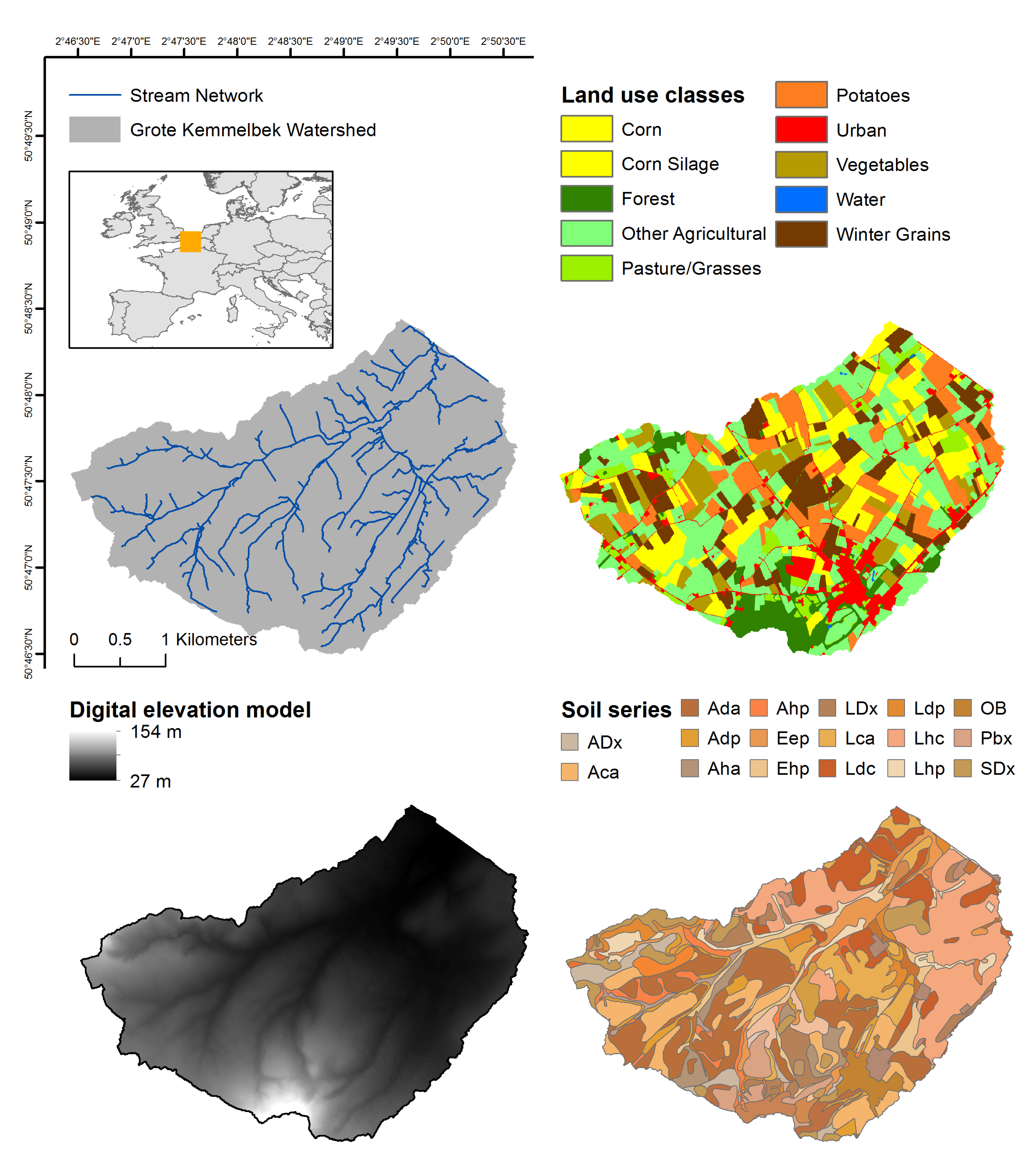
The GKb catchment is located in the Flanders region of Belgium (see
Figure 1) with an area of approximately 1030 ha. The catchment’s land use is predominantly agricultural (>85%), with some forest, farmsteads, and non-cultivated grassland. Main crops grown include corn, potato, and winter wheat. Agricultural fields are close to surface water bodies (i.e., no riparian buffers). The mean elevation of the catchment is 53 m, and ranges from a minimum of 27 m to a maximum of 154 m. Based on the years from 2010 to 2013, the average annual precipitation for the GKb catchment is 815 mm/year, with 18 mm/year (liquid equivalent) falling as snow or frozen precipitation. The watershed soils are mostly poorly to imperfectly drained loams, silts, and silt loams, and about 50% of the watershed area is tile-drained.
2.3. Input Data Sets
2.3.1. Spatial Input Data
Figure 1 gives an overview of the GKb stream network, topography, land use, and soil type distributions. A digital elevation model (DEM) with a resolution of 1 m [
19] was resampled to a resolution of 2 m and used for landscape and watershed delineation. Physical soil properties were extracted from a 1:20,000 soil survey [
18] and the Land Use and Coverage Area frame Survey (LUCAS, [
20]). A land-use data spatial data layer for the GKb catchment was developed from four years of field-specific cropping information collected as part of the monitoring and stewardship program in the catchment [
21]. The annual maps from the stewardship program were filled up with OSM (Open Street Map) land use data to provide a continuous land use layer. A spatial data layer of streams along with a survey of stream cross-section geometry was obtained from the Flemish government and the municipality Heuvelland via personal communication. The data was used to burn the channel network into the DEM and define SWAT channel parameters. An overview of the input data is provided in
Table 1.
2.3.2. Farmer Survey Application Data
Pesticide application data and other agronomic data (e.g., planted crops) were obtained by carrying out a field-level survey among the farmers within the catchment area after each growing season [
21]. Based on this survey, applied herbicides, application rates, and dates were provided for each field along with information on crop rotations. All this data was compiled into field-specific management schedules. Furthermore, the data was used to derive more generic information such as percent crop treated, average application rates, and typical application windows. An overview of the annually cropped and FFA treated acreage within the GKb catchment is provided in
Table 2.
2.3.3. Weather
Daily precipitation and temperature data (required for the Hargreaves potential evaporation method) were obtained from 4 gauges outside of the watershed area. Virtual gauges were created for each subbasin based on an inverse distance interpolation method.
2.3.4. Monitoring Data
A monitoring station measuring flow was set up at the outlet of the GKb catchment for a period of 3.5 years (May 2010 to December 2013). Two daily water samples were collected and analyzed for pesticide residues over the same period and location as the streamflow monitoring. The high-resolution flow and concentration data were aggregated to daily average values for use in calibration and evaluation of the SWAT+ model. There was one notable period of missing data (from 5–29 March 2012) when a high flow event damaged the flow monitoring equipment. Details regarding the monitoring program are provided in [
21]. The hydrograph is shown in the
Section 3.
This study focused on the herbicide flufenacet (FFA) and its metabolite FFA-SA, which both have been the objective of other pesticide exposure studies [
24]. Typical applications of FFA occurred in the GKb catchment between April and June, and significant concentrations were observed at the monitoring station in May 2010 (5.1 µg/L), and June–July 2012 (2.055 to 3.845 µg/L). FFA, with moderate mobility, tends to peak within its application period or shortly after and disappears relatively quickly after the application period. In contrast, FFA-SA is a degradate of FFA that forms through aerobic soil metabolism [
25]. It peaks about six months after the FFA application period and had its maximum observed concentrations in December 2011 (1.07 µg/L) and October 2013 (1.04 µg/L). The observed FFA and FFA-SA monitoring data is shown in the
Section 3.
2.3.5. Environmental Fate Properties
The FFA and FFA-SA environmental fate characteristics were the same as used in the EU regulatory process [
25]. These parameters include a soil adsorption coefficient (K
oc) of 221.2 mg/L, a soil half-life of 12.12 days, a foliar half-life of 3 days, no aerobic aquatic degradation, and an anaerobic aquatic half-life of 49.6 days for FFA. For the metabolite FFA-SA, a soil adsorption coefficient (K
oc) of 11.1 mg/L, a soil half-life of 31.62 days, and no aerobic and anaerobic aquatic degradation were used. FFA-SA only forms from FFA through soil metabolism processes with a formation fraction of 0.247.
2.4. FFA Point Source Contributions in the GKb
During the course of the stewardship program [
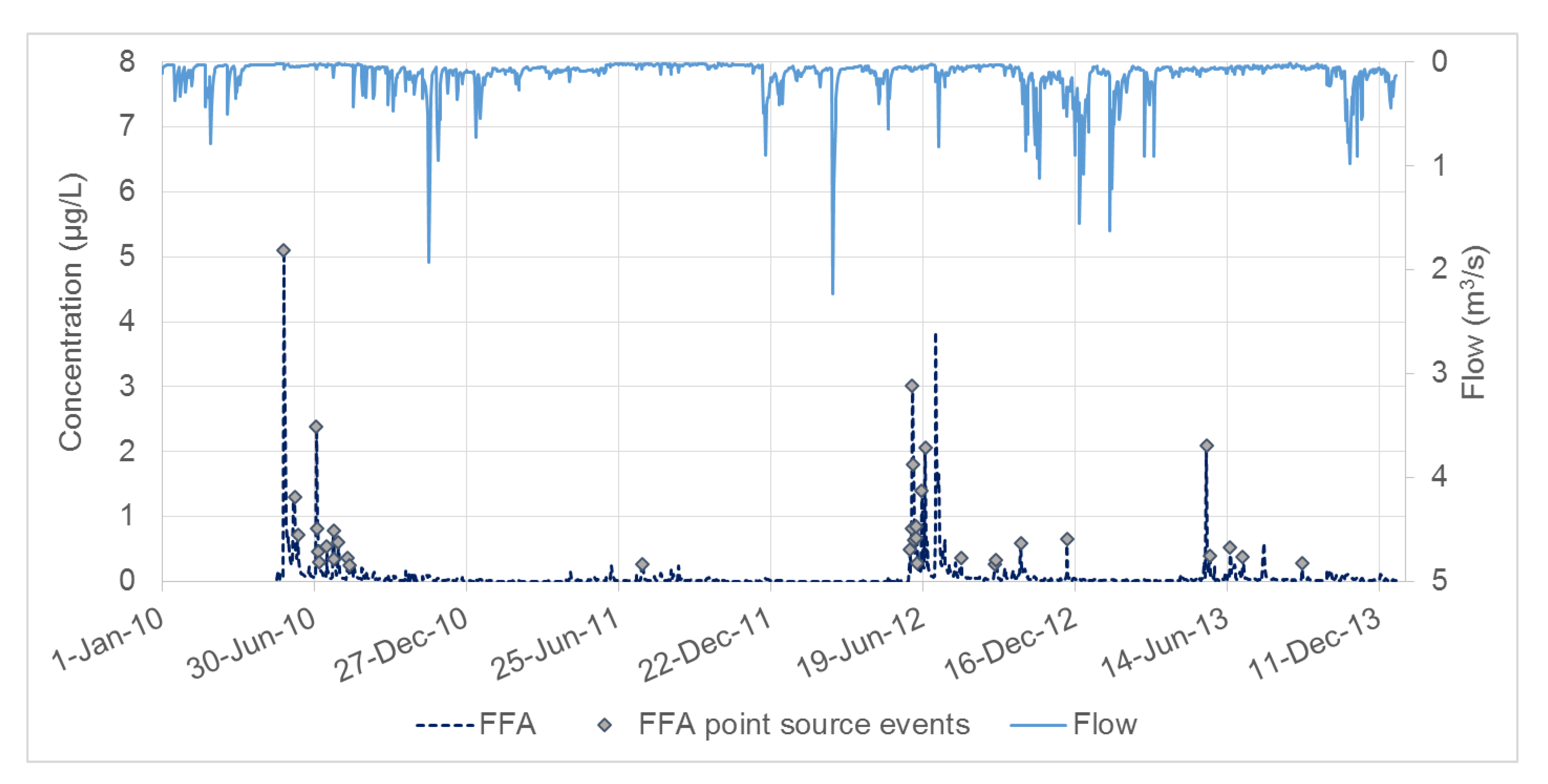
21], it was determined that misuse of the products (e.g., spillage on hard surfaces during filling or wash-off from rinsing spraying equipment) caused pesticide point source contributions to surface waters in the GKb. This was confirmed by a modelling study conducted by [
26]. The analysis found that 46% (34 of 74) of elevated FFA concentration detections (greater than 0.25 µg/L) were not likely to be caused by diffuse sources and were therefore likely to be a result of point-source contributions (see
Figure 2 below and Figure 2 in [
26]). The identification of the point source contributions is important for understanding exposure pathways and developing effective mitigation measures. From a modeling perspective, the information is crucial because without the identification of point source contributions unrealistic parameter values might be determined during the calibration process or wrong conclusions might be drawn regarding the model performance.
2.5. Baseline SWAT+ Setup and Parametrization
Several model configurations were needed to fulfill the research objectives of this study. However, in the first step, a baseline configuration was set up using the input data described above. The baseline configuration is supposed to represent the most realistic configuration and was used for model calibration. It takes advantage of the landscape-level transport processes (landscape routing) and uses the pesticide application data provided by the farmer survey. Simulations were conducted for the 4-year period from 2010 to 2013 that overlaps with the period for which monitoring data is available, plus a 2-year warm-up period from 2008 to 2009.
The QSWAT+ interface (available through the SWAT+ website) was used for watershed and landscape unit delineation. Two landscape units representing upland and floodplain areas were defined using the inverted DEM slope position method [
10] with a slope position threshold of 0.1. Among the methods and thresholds tried, this configuration resulted in floodplain areas that had the best fit with poorly to very poorly drained soils and gleysols. In total, 23.7% of the total watershed area was defined as a floodplain. Connectivity between upland, floodplain, and channel was set up according to the method suggested by [
14]. A deep aquifer was added to the default interface configuration which is an established method to better account for the complex subsurface processes in lowland catchments [
27]. The field-level land use data and detailed stream network resulted in 505 landscape units and 6419 HRUs.
Each FFA application was realized with a management operation designed specifically to replicate a foliar spray application as parametrized in the United States Environmental Protection Agency (USEPA) Pesticide Root Zone Model (PRZM) 3.12.2 [
28], which is used for US and EU regulatory pesticide exposure modeling. In this approach, the pesticide is incorporated down to 4 cm (with the incorporated mass linearly decreasing with depth). To this end, 43.75% of the chemical mass is surface applied and the remaining fraction is injected at a depth of 20 mm. An application efficiency of 99% was assumed. Off-target drift deposition onto the surface water bodies was not considered in this study.
2.6. Model Calibration
The SWAT model was calibrated to the observed flow, FFA, and FFA-SA concentration data. The calibration of the three components was conducted concurrently while the evaluation approach differed between hydrologic and chemical calibration. The hydrologic component included both a quantitative evaluation of goodness-of-fit statistics and a qualitative assessment of hydrograph attributes (shape and timing). The goodness-of-fit statistics included the PBIAS (percent bias), NSE (Nash Sutcliffe Efficiency, [
29]), logNSE (logarithm of the NSE to emphasize low flows), and KGE (Kling-Gupta Efficiency, [
30] based on [
31]). Due to the FFA point source contribution issue described above, FFA was evaluated qualitatively based on the concentration probability exceedance distribution and shape and timing of the chemograph. Because FFA-SA is not subject to the point source situation, the NSE was calculated on the probability exceedance curve using 1% increments in addition to the qualitative evaluation. The adjustment of parameters was conducted manually. A manual calibration approach was followed in favor of an automatic optimization approach to achieve a better understanding of the catchment’s hydrology and transport processes represented by SWAT+. While implementing an automatic optimization approach likely could have achieved somewhat better goodness-of-fit statistics, the benefits of the manual approach were judged to be of higher value. The entire 3.5-year record of observed data was considered to be the calibration period, and a second independent validation period was not selected. This is a common approach used for hydrologic model calibration when the observed data period is too short [
32].
The parameters selected for calibration and their final version are shown in
Table 3. It should be noted that the FFA and FFA-SA soil half-life values were adjusted to account for the difference between the laboratory and actual temperature in the watershed. To this end, the range of realistic half-life values was determined using the Q10 factor method as described in [
33]. The final values of 24.24 and 55.34 days for FFA and FFA-SA, respectively, represent a temperature-adjusted decay which is still in the range of the laboratory values reported in [
25].
2.7. Analysis Framework
The three objectives of this study were to (1) assess if SWAT+ is capable of concurrently simulating a pesticide and one of its metabolites, (2) evaluate and estimate the impact of the new landscape level spatial representation of pesticide transport processes, and (3) evaluate the rule-based probabilistic pesticide application approach. To this end, two watershed configurations with landscape routing (LR) and without landscape routing (NR) were created along with five different pesticide application schedule realizations based on the farmer survey (FS) or SWAT+’s conditional management approach (C1 to C3B).
The application scenarios were developed to evaluate whether the SWAT+ rule-based probabilistic pesticide application approach results in similar pesticide concentrations compared to what is achieved using detailed field-level application data available from a farmer survey. The conditional scenarios assumed that only basic information regarding pesticide applications is available. This includes the typical number of applications within the growing season, the average application rate per crop, the percent crop treated (PCT), and a range of dates on which the pesticide is applied (an application window). The conditional applications include a random component and require running and evaluating an ensemble of simulations (e.g., 100 runs) to avoid biases. In this study, the evaluation showed no systematic bias, and a random run was selected for a detailed evaluation which is presented here.
The list below describes the seven setups designed to address the three research objectives of this study. Each configuration is labeled by a letter code in the form of XX-YY, where XX specifies the landscape configuration (NL or LR) and YY indicates which agricultural management scenario was used, farmer survey-based (FS) or conditional operations (C1 to C3B). The different configurations are summarized in
Table 4.
LR-FS—Landscape routing with farmer survey-based pesticide applications. This configuration is the baseline simulation used for calibration and represents the highest degree of realism in terms of transport processes and pesticide applications. Evaluation of the landscape pesticide transport processes and the metabolite formation and transport is conducted based on this setup.
NL-FS—No landscape routing with farmer survey-based pesticide applications. This configuration is a clone of LR-FS but without considering interactions between upland and floodplain landscape units. Flow and loadings originating in the upland are routed directly to the channel system. This setup represents the classic SWAT-HRU configuration. A comparison between this setup and LR-FS is used to assess the impact of landscape routing for pesticide exposure assessments.
LR-C1—Landscape routing with conditional pesticide applications 1. The following configurations represent different complexities of conditional management operations, where a pesticide application is triggered by certain rules. More realism is incorporated into the rules in a stepwise approach to assess the impact of individual refinement steps. The C1 scenario represents the simplest ruleset where 100% of the crops on the FFA label are treated (PCT of 100%) on a single day (mid-point of the typical application window), with a typical application rate. Assuming a pesticide is applied to all cropped areas is a common assumption in conservative pesticide exposure modeling scenarios (e.g., screening level simulations) and when no pesticide usage data is available.
LR-C2A—Landscape routing with conditional pesticide applications 2A. The C2 scenario accounts for actual usage instead of assuming 100% PCT. In this scenario, HRUs are randomly selected by the SWAT+ conditional module for being treated with FFA based on the likelihood represented by the PCT. All applications are still made on a single day.
LR-C2B—Landscape routing with conditional pesticide applications 2B. The 2B scenario represents the actual PCT through PCT adjusted application rates. This means that all crops are treated with a PCT-adjusted application rate (i.e., the typical application rate is multiplied by the PCT). The pesticide mass applied within the watershed is the same for scenarios 2A and 2B.
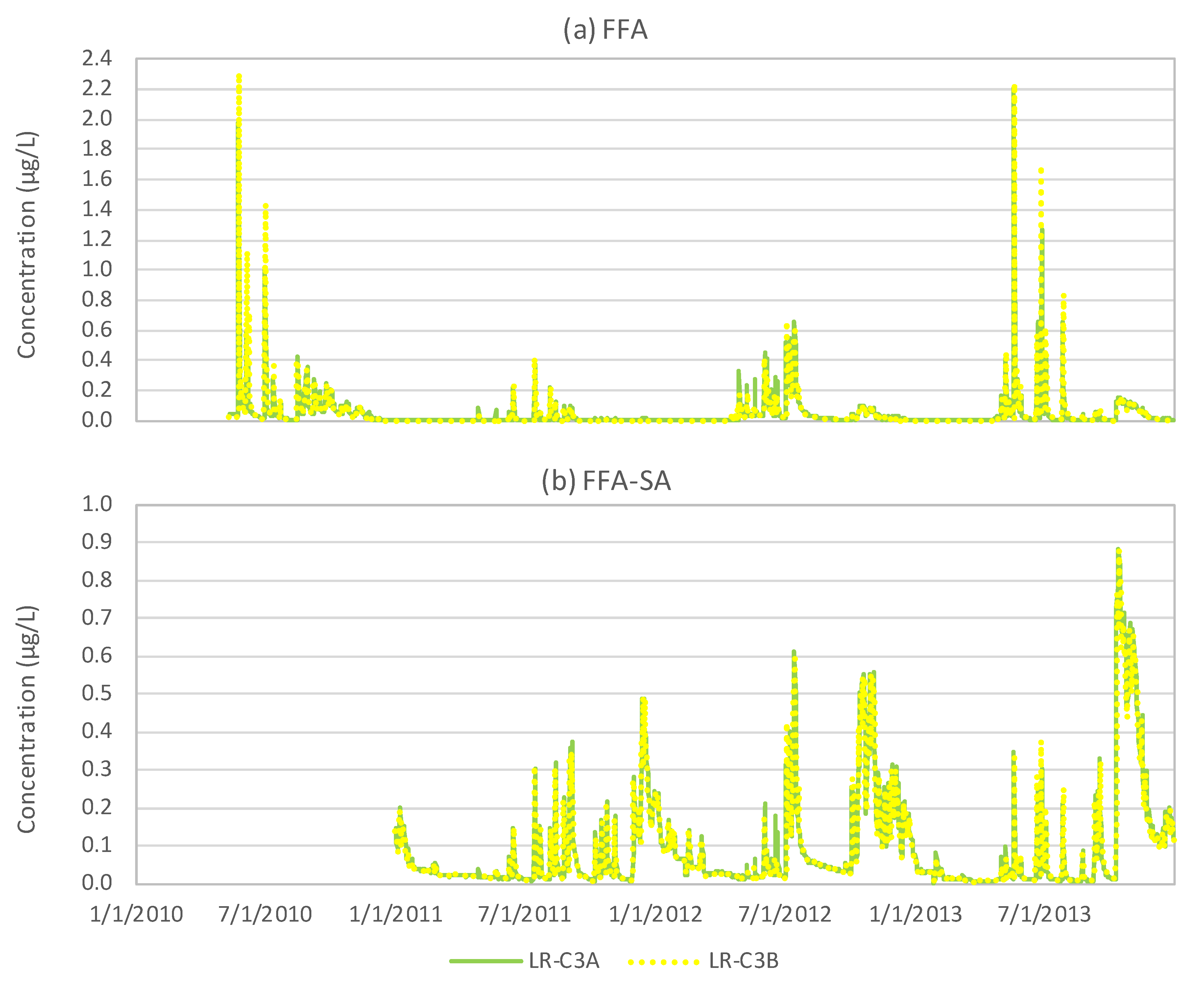
LR-C3A—Landscape routing with conditional pesticide applications 3A. This scenario uses the same configuration as in C2A, but the applications are spread out over a typical application period, resulting in applications throughout the watershed occurring on many different dates. The selection of which HRUs are treated on which date is automatically conducted by SWAT+’s conditional module by assuming a uniform distribution of the application window.
LR-C3B—Landscape routing with conditional pesticide applications 3B. This scenario uses the same configuration as in C2B, but the applications are spread out over a typical application period resulting in applications throughout the watershed occurring on many different dates. The selection of which HRUs are treated on which date is automatically conducted by SWAT+’s conditional module.
3. Results and Discussion
3.1. Model Calibration and Evaluation of Chemical Transport Processes
Table 5 shows the basin water balance and pesticide budgets. The distribution of the flow components and the relevance of these pathways for the associated FFA and FFA-SA transport indicate that tile and lateral flow in the GKb catchment contribute most to streamflow, which are also the most significant transport pathways for both, FFA and FFA-SA. Surface runoff and groundwater flow components are in a similar range. However, surface runoff has a higher relevance for FFA transport and groundwater flow for FFA-SA.
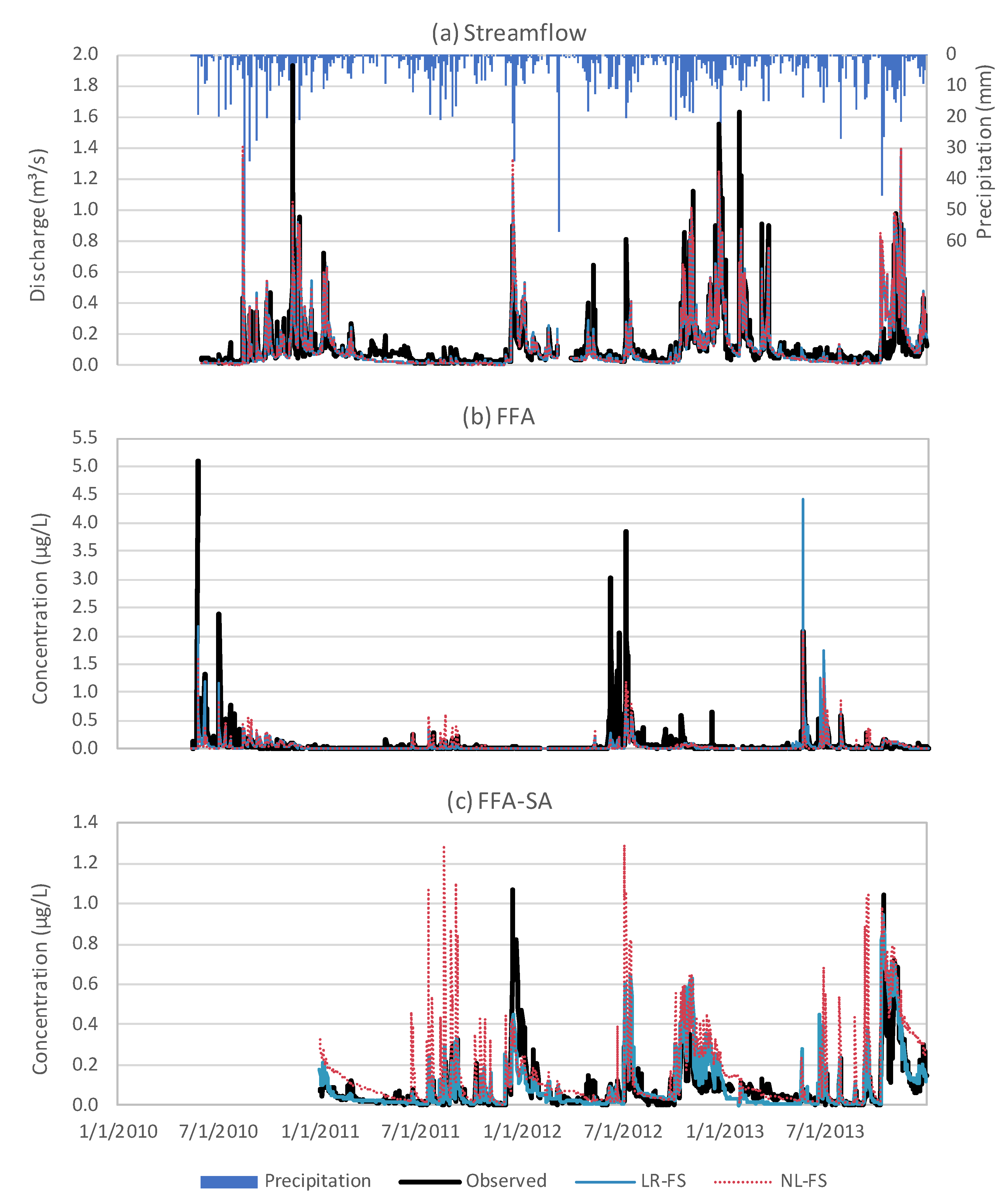
The daily hydrograph for the calibration scenario FS-LR (see
Figure 3a) indicates that the model simulates daily streamflow well in both, low and high flow conditions. The model, however, tends to underpredict discharge peaks. During the simulation period, annual precipitation in the GKb catchment varies between 634 mm (2011) and 944 mm (2012). The high variability in precipitation provides a challenge for model calibration and discrepancies in peak flows are common for SWAT in such conditions [
9]. Nevertheless, the values of typically used model performance metrics are very good according to [
34]. The PBIAS, daily NSE, and daily KGE are 3.26%, 0.63, and 0.81 over the entire simulation period and it was concluded that the hydrologic model performance provides a good foundation for evaluating chemical transport and formation processes.
Reviewing the daily FFA chemograph (
Figure 3b) shows that the model is able to accurately predict the dynamics and timing of pesticide concentrations but tends to underpredict extreme events in 2010 and 2012, while such events are overpredicted in 2013. The underprediction can be partly attributed to the fact that the model also underpredicts streamflow peaks and associated surface runoff-related transport processes. It should further be noted that the daily monitoring concentration data was calculated as the average from multiple daily samples [
21] while the simulated concentration is obtained from a daily time-step model. Thus, the model might not capture the peak concentration seen in the monitoring data due to the different time scales used for modeling and monitoring, which could further explain the underestimation of some peak events. However, for the FFA evaluation, it should be kept in mind that previous research showed that 46% of elevated FFA concentrations greater than 0.25 µg/L are likely caused by point sources [
26] as they could not be explained with diffuse physical transport processes (
Figure 2). The FFA concentration overprediction in 2013 could be caused by two consecutive high precipitation years that lead to high soil moisture conditions in the model causing an overestimation of pesticide transport into the channel via surface runoff and fast subsurface processes. Precipitation in 2012 and 2013 was 943 mm and 878 mm, respectively while the mean precipitation is 815 mm.
The ability to directly simulate the formation of metabolites was integrated into SWAT+ by the SWAT+ development team during this research effort and the evaluation of those processes was part of the scope of this study. The simulated FFA-SA daily chemograph (
Figure 3c) shows very good agreement with the observed chemograph. Considering the overall low concentrations, the predictions of the peak concentrations are accurate (with one exception in 2011). The chemograph is well represented during peak, recession, and low concentration periods, which is confirmed by the probability exceedance curve shown in
Section 3.3 (Conditional Management Operations) and the corresponding NSE of 0.99.
3.2. Impact of Landscape Routing
The differences in streamflow at the GKb outlet between the landscape (LR-FS) and no-landscape routing (NR-FS) scenario were small (see
Figure 3a) with minimal differences during low-flow periods. For some events, the peaks of the NL-FS routing scenario were greater than the peaks of the LR-FS scenario. A fraction of the runoff generated in the upland interacts with the floodplain and has the opportunity to infiltrate into the floodplain, which has a buffering effect on the peaks. However, for other events, it can be observed that the landscape routing scenario shows higher peaks. Those events mainly occur during the wet season. At that point, the soil moisture in the floodplain landscape unit is more saturated and has little capacity for infiltration of precipitation falling on the floodplain and runoff from the upland. Precipitation on the more saturated landscape results in higher surface runoff, which explains the higher peak of the landscape routing scenario during those conditions.
Comparing the observed, LR-FS, and NR-FS FFA chemograph shows that the differences between the routing schemes at the GKb outlet are small (see
Figure 3b). The LR scenario shows greater peak concentrations and is closer to the observed values than the NL configuration. However, this observation is not 100% consistent and there are some events (e.g., in July 2012) where the NL shows higher peaks. As FFA is primarily surface runoff driven, the explanation given for streamflow above also applies to FFA concentrations. The point source contribution issue described above impedes an impartial comparison between observed and simulated values. However, the spatially more realistic LR setup seems to provide more realistic results at the GKb outlet.
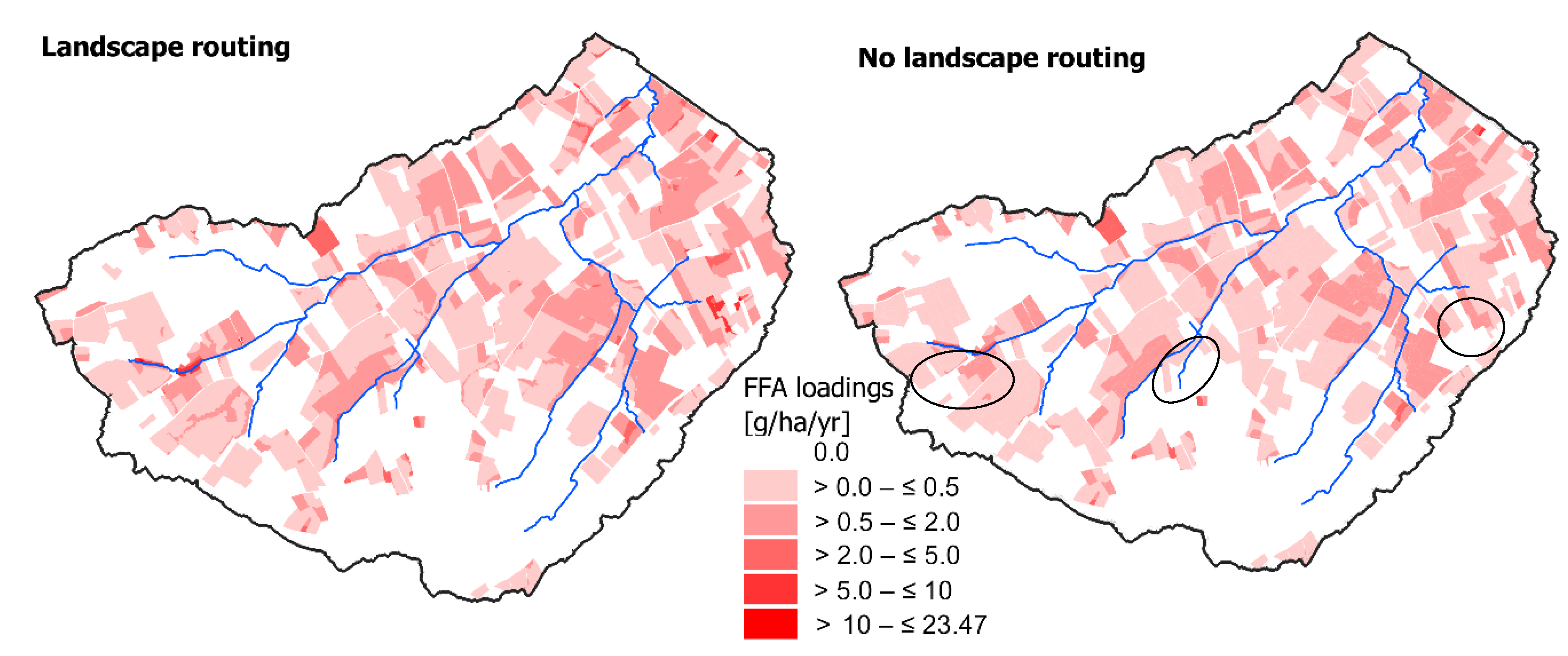
A comparison of the spatial distribution of annual average HRU-level FFA loadings between the LR-FS and NR-FS scenarios shows that the landscape routing setup provides a more realistic configuration. Some fields located in close proximity to the streams show a higher vulnerability (based on FFA loadings) compared to the no-landscape setup (
Figure 4). If the modeler’s scope is a spatial description of pesticide transport processes within a hydrologic system (e.g., detection of critical pesticide source areas), the spatially more realistic landscape routing configuration is recommended, because spatial patterns of topography and subsurface characteristics often exert significant control over hydrological processes within a watershed [
11].
Comparing the FFA-SA chemographs (see
Figure 3c) further highlights the importance of a spatially more accurate routing scheme. The LR-FS shows a good agreement between observed and simulated FFA-SA concentrations, while the NR-FS setup overpredicts most concentration peaks and shows higher discrepancies to the observed values during recession and low-flow periods. However, it should be noted that calibration was conducted on the LR-FS configuration and that outperformance of the LR-FS over the NR-FS model is expected. Nevertheless, differences between the setups at the outlet were relatively minor for streamflow and FFA concentrations, while bigger differences are observed for FFA-SA concentrations. This is confirmed by the probability exceedance distributions shown in
Figure 5d. The corresponding NSE values calculated on the exceedance curve are 0.99 and 0.90 for the LR-FS and NR-FS models, respectively. The results demonstrate that a realistic routing scheme is an important factor in pesticide risk assessments. The benefit of a more accurate simulation of the landscape and the availability of model output with a higher spatial resolution comes at the cost of increased model complexity that leads to higher computational demands.
3.3. Conditional Management Operations
An evaluation of the rule-based management applications for FFA and FFA-SA is presented in
Figure 5. For FFA (
Figure 5a) it can be seen that the rule-based management applications converge towards the most realistic (LR-FS) simulation with an increasing level of realism incorporated into the management rules (LR-C1 to LR-C3A). The rule-based management operations are able to represent the concentration dynamics well and the timing of events is similar to the farmer-survey-based applications. The simplest rule-based applications (LR-C1) overestimate peak concentrations in comparison to LR-FS. The greatest level of refinement was achieved when incorporating actual usage information in the form of annual crop-specific PCT values (LR-C2A). Spreading out the applications over a time window results in further reductions of concentrations but also leads to events that are not seen in the observed data or in the LR-FS simulations. This is expected because the conditional timing of applications includes a random component leading to applications that did not necessarily reflect reality.
The most refined conditional simulation (LR-C3A) matches the peaks predicted by LR-FS well in most cases. However, there are one major and two minor peaks in 2013 where the LR-C3A model underestimates the concentration magnitude of LR-FS. Such differences can be caused by the fact that actual location, timing, and application rates are used by LR-FS, while LR-C3A uses randomly selected fields with a random timing and an average application rate. For the conditional simulations, it was also evaluated whether it makes a difference to (a) randomly treat HRUs (or fields) according to the PCT or (b) treat all HRUs (or fields) but adjust the application rate by the PCT. The evaluation shows that there are minor differences between the two options and that both options generate feasible results (
Figure 6).
A first look at the exceedance probability plot shown in
Figure 5c unexpectedly indicates that the simple (LR-C1) scenario agrees best with the observed and farmer survey-based simulation (LR-FS). However, the good agreement between the LR-FS simulation and the observed data for the extreme event is mainly caused by an LR-FS overprediction in 2013 that matches the magnitude of an observed event in early 2010, which is under predicted. For less extreme events (from the greater 1% to 100% exceedance probability) the LR-FS, LR-C2A, and LR-C3A distributions agree very well. Overall, it can be concluded that the stepwise incorporation of realism into SWAT+ conditional management operations resulted in lower predicted exposure concentrations. The conditional simulations are able to produce concentrations similar to what can be achieved with farmer survey-based application data. However, the FFA point source contribution issue makes an evaluation challenging.
Comparing the conditional simulations for FFA-SA shows that the most refined rule-based simulation agrees best with the LR-FS scenario and observations (
Figure 5b,d). The FFA-SA concentrations are not subject to the FFA point source contribution issue. There are, however, some events with a discrepancy between LR-C3A and LR-FS FFA-SA peak concentrations (e.g., in July 2013). The FFA-SA exceedance probability curve shows a very good match between observed, LR-C2A, LR-C3A, and LR-FS simulations. The NSE calculated on the exceedance probability distribution is 0.88 for LR-C1 and 0.99 for LR-C2A, LR-C3A, and LR-FS. Similar to what was observed for FFA, the difference between using the actual PCT with an average application rate (LR-C2A and LR-C3A) and using 100% PCT with a PCT-adjusted application rate (LR-C2B and LR-C3B) are relatively minor and no difference can be seen in the NSE applied to the exceedance probability distribution. In summary, the results for FFA and FFA-SA show that rule-based applications can be used as a surrogate for field-level farmer survey-based pesticide application information. While the conditional simulation cannot predict individual events, the overall dynamics and annual magnitude of events are well represented, especially for FFA-SA.
4. Summary and Conclusions
The next generation of the SWAT model, SWAT+, was applied and evaluated in terms of its suitability for pesticide concentration time series and daily exceedance probability predictions. SWAT+ provides three main advantages for pesticide risk assessments over the SWAT model, which are (1) the ability to directly simulate the formation of degradation compounds, (2) spatially more explicit representation of hydrologic and chemical transport processes, and (3) the availability of more flexible, rule-based management operations well-suited to describing pesticide application practices at the watershed scale. This paper evaluated the functionality of the three new features and assessed their impact on pesticide exposure simulations. The GKb catchment was chosen as a study area because 3.5 years of high-resolution monitoring data were available together with a field-level farmer survey where all herbicide applications were reported. The evaluation was based on the commonly used herbicide FFA and its soil metabolite FFA-SA.
The hydrologic and chemical calibration was conducted using the spatially more explicit landscape routing configuration and FFA applications based on the field-level farmer survey. It resulted in very good hydrologic, satisfactorily FFA, and very good FFA-SA performance. Despite some challenges related to the FFA point source contribution issue in the GKb catchment, the results obtained here confirm that SWAT+ has the capability for accurate watershed-scale pesticide simulations, as has also been observed in numerous studies for the original SWAT model. SWAT+ showed very good performance in simulating the metabolite FFA-SA, demonstrating that SWAT+ is able to simulate the formation of degradation compounds which fills a gap in the currently available toolset of watershed scale pesticide exposure assessments.
Evaluation of a more accurate spatial representation of hydrologic and chemical transport processes was conducted based on two setups which were both based on the farmer survey applications. The setups were identical, except for the routing scheme used. The results showed (1) a minimal impact of the routing scheme on hydrology, (2) that more realistic pesticide concentrations could be obtained with the landscape routing setup at the watershed outlet, and (3) that the landscape routing setup provides higher resolution spatial information important for the identification of critical pesticide source areas. The benefit of the landscape routing was more significant for the metabolite FFA-SA while the FFA evaluation remained challenging due to the point source contribution issue. It should be noted that calibration was conducted on the landscape routing setup, which might have introduced a bias that caused the outperformance of the landscape routing setup over the non-landscape routing setup. However, the spatial evaluation and the higher difference of FFA-SA concentrations between the two setups shows the importance of an accurate representation of transport processes for pesticide exposure assessments. Future research should be conducted to confirm the importance of the landscape position (e.g., distance to surface water bodies) for the environmental impact of pesticide applications.
The absence of pesticide application data (location, timing, rate) is a major uncertainty in most pesticide exposure assessments. Such data is only available through farmer surveys, which are time consuming and expensive to conduct. Thus, it was evaluated whether SWAT+’s conditional management operations can provide results similar to what can be obtained from field-level application information. The most refined rules evaluated in this study require annual percent crop treated (PCT) values, a typical application rate, and a typical application window. That information is often available through market surveys and crop consultants. The results of this study indicate that individual events cannot be accurately simulated with that approach but that a similar degree of realism can be achieved if this information is used in SWAT+ rule-based management operations, which would reduce the costs for farmer surveys. However, the benefit could come at the cost of greater model uncertainty when the parameters required for rule-based scheduling (PCT, application rate, application window) are estimated. Future studies are needed to confirm the findings and develop guidance on how to derive these parameters.
It was further evaluated whether there is a difference between using actual PCT with a typical application rate or assuming a PCT of 100% with a PCT-adjusted application rate. While both setups result in the same mass of pesticide applied in the watershed, the actual PCT requires a random selection of fields being treated. The results from this study indicate that the choice of method does not have a significant impact on simulating the timing and magnitude dynamics of pesticides and their metabolite, but that there can be differences for individual events. Using the PCT-adjusted rate is recommended for a critical source area analysis as it accounts for the entire treatable area and avoids a random selection of treated areas.
The accuracy of the pesticide concentration simulations with the new features of SWAT+ in the present study demonstrates the model’s ability to provide more predictive estimates with reduced uncertainty. In addition to the extensive peer-revision and testing by the international scientific community, our evaluation of SWAT+ and its new features further supports the model viability for regulatory pesticide exposure assessment use.
Author Contributions
Conceptualization, H.R., M.W. and R.S.; Data curation, J.K., M.B.M., M.W. and R.S.; Methodology, H.R., J.K. and M.W.; Software, J.G.A.; Supervision, R.S.; Validation, J.K., H.R., M.W. and R.S.; Visualization, J.K., M.B.M. and H.R.; Funding acquisition, R.S.; Writing—original draft, H.R.; Writing—review & editing, J.K., M.W., R.S. and J.G.A. All authors have read and agreed to the published version of the manuscript.
Funding
We acknowledge and thank Bayer AG Division Crop Science for funding the work.
Institutional Review Board Statement
Not applicable.
Informed Consent Statement
Not applicable.
Data Availability Statement
The data presented in this study are available on request from the corresponding author. The data are not publicly available because some of the model input and monitoring data is proprietary.
Conflicts of Interest
The authors declare that they have no known competing financial interests or personal relationships that could have appeared to influence the work reported in this paper.
References
- Stehle, S.; Bub, S.; Schulz, R. Compilation and analysis of global surface water concentrations for individual insecticide compounds. Sci. Total Environ. 2018, 639, 516–525. [Google Scholar] [CrossRef] [PubMed]
- Willkommen, S.; Pfannerstill, M.; Ulrich, U.; Guse, B.; Fohrer, N. How weather conditions and physico-chemical properties control the leaching of flufenacet, diflufenican, and pendimethalin in a tile-drained landscape. Agric. Ecosyst. Environ. 2019, 278, 107–116. [Google Scholar] [CrossRef]
- Quilbé, R.; Rousseau, A.N.; Lafrance, P.; Leclerc, J.; Amrani, M. Selecting a Pesticide Fate Model at the Watershed Scale Using a Multi-criteria Analysis. Water Qual. Res. J. 2006, 41, 283–295. [Google Scholar] [CrossRef]
- Arnold, J.G.; Srinivasan, R.; Muttiah, R.S.; Williams, J.R. Large-area hydrologic modeling and assessment: Part I. model development. Am. Water Res. 1998, 34, 73–89. [Google Scholar] [CrossRef]
- Winchell, M.F.; Peranginangin, N.; Srinivasan, R.; Chen, W. Soil and Water Assessment Tool model predictions of annual maximum pesticide concentrations in high vulnerability watersheds. Integr. Environ. Assess. Manag. 2018, 14, 358–368. [Google Scholar] [CrossRef] [PubMed] [Green Version]
- Gassman, P.W.; Reyes, M.R.; Green, C.H.; Arnold, J.G. The Soil and Water Assessment Tool: Historical development, applications, and future research directions. Trans. ASABE 2007, 50, 1211–1250. [Google Scholar] [CrossRef] [Green Version]
- Arnold, J.; Allen, P.; Volk, M.; Williams, J.; Bosch, D. Assessment of different representations of spatial variability on SWAT model performance. Trans. ASABE 2010, 53, 1433–1443. [Google Scholar] [CrossRef]
- Bosch, D.D.; Arnold, J.G.; Volk, M.; Allen, P.M. Simulation of a low-gradient coastal plain watershed using the SWAT landscape model. Trans. ASABE 2010, 53, 1445–1456. [Google Scholar] [CrossRef]
- Rathjens, H.; Oppelt, N.; Bosch, D.D.; Arnold, J.G.; Volk, M. Development of a grid-based version of the SWAT landscape model. Hydrol. Process. 2015, 29, 900–914. [Google Scholar] [CrossRef]
- Schulz, K.; Seppelt, R.; Zehe, E.; Vogel, H.J.; Attinger, S. Importance of spatial structures in advancing hydrological sciences. Water Resour. Res. 2006, 42, 1–4. [Google Scholar] [CrossRef] [Green Version]
- Rathjens, H.; Bieger, K.; Chaubey, I.; Arnold, J.G.; Allen, P.M.; Srinivasan, R.; Bosch, D.D.; Volk, M. Delineating floodplain and upland areas for hydrologic models: A comparison of methods. Hydrol. Process. 2016, 30, 4367–4383. [Google Scholar] [CrossRef]
- Bieger, K.; Arnold, J.G.; Rathjens, H.; White, M.J.; Bosch, D.D.; Allen, P.M.; Volk, M.; Srinivasan, R. Introduction to SWAT+, A completely Restructured Version of the Soil and Water Assessment Tool. J. Am. Water Resour. Assoc. 2016, 53, 115–130. [Google Scholar] [CrossRef]
- Nkwasa, A.; Chawanda, C.J.; Jägermeyr, J.; van Griensven, A. Improved representation of agricultural land use and crop management for large-scale hydrological impact simulation in Africa using SWAT+. Hydrol. Earth Syst. Sci. 2022, 26, 71–89. [Google Scholar] [CrossRef]
- Bieger, K.; Arnold, J.G.; Rathjens, H.; White, M.J.; Bosch, D.D.; Allen, P.M. Representing the Connectivity of Upland Areas to Floodplains and Streams in SWAT+. J. Am. Water Resour. Assoc. 2019, 55, 578–590. [Google Scholar] [CrossRef]
- Arnold, J.G.; Bieger, K.; White, M.J.; Srinivasan, R.; Dunbar, J.A.; Allen, P.M. Use of Decision Tables to Simulate Management in SWAT+. Water 2018, 10, 713. [Google Scholar] [CrossRef] [Green Version]
- Leonard, R.R.; Kmisel, W.G.; Still, D.A. GLEAMS: Groundwater loading effects of agricultural management system. Trans. ASAE 1987, 30, 1403–1418. [Google Scholar] [CrossRef]
- Chapra, S.C. Surface Water-Quality Modeling; WCB.McGraw-Hill: Boston, MA, USA, 1997. [Google Scholar]
- DOV. Spatial and Tabular Soil Data Base. (Databank Ondergrond Vlaanderen). Available online: https://www.dov.vlaanderen.be (accessed on 1 June 2020).
- Geopunt. Digital Elevation Model in 1 m Resolution, Flemish Geodata Portal. Available online: https://www.geopunt.be/ (accessed on 5 May 2020).
- Joint Research Centre and Institute for Environment and Sustainability. LUCAS Topsoil Survey: Methodology, Data and Results; Montanarella, L., Jones, A., Tóth, G., Eds.; Publications Office of the European Union: Luxembourg, 2013; pp. 1–154. [Google Scholar] [CrossRef]
- Baets, D.; Sur, R.; Krebber, R.; Lembrich, D. High-Resolution Water Monitoring Program Gives Further Insights on Sources of Residues from Herbicides in Surface Water. Commun. Agric. Appl. Biol. Sci. 2019, 83, 326–335. [Google Scholar]
- Saxton, K.E.; Rawls, W.J.; Romberger, J.S.; Papendick, R.I. Estimating Generalized Soil-water Characteristics from Texture. Soil Sci. Soc. Am. J. 1986, 50, 1031–1036. [Google Scholar] [CrossRef]
- Saxton, K.; Willey, P. The SPAW model for agricultural field and pond hydrologic simulation. Model. Watershed Hydrol. 2006, 300, 401–435. [Google Scholar] [CrossRef]
- Willkommen, S.; Lange, J.; Ulrich, U.; Pfannerstill, M.; Fohrer, N. Field insights into leaching and transformation of pesticides and fluorescent tracers in agricultural soil. Sci. Total Environ. 2021, 751, 141658. [Google Scholar] [CrossRef]
- Bayer Crop Science. Flufenacet (FFA) and metabolites: Use in winter cereals in Europe. Bayer Crop Sci. Intern. Rep. 2018, 1, 144. [Google Scholar]
- Sur, R.; Winchell, M.; Rathjens, H.; Baets, D.; Krebs, F.; Lembrich, D. Identification of Herbicide Source Areas and Exposure Pathways in a Watershed Based on Landscape Modeling and High-Resolution Monitoring Data. Commun. Appl. Biol. Sci. 2018, 83, 336–340. [Google Scholar]
- Pfannerstill, M.; Guse, B.; Fohrer, N. A multi-storage groundwater concept for the SWAT model to emphasize nonlinear groundwater dynamics in lowland catchments. Hydrol. Process. 2013, 28, 5599–5612. [Google Scholar] [CrossRef]
- Suaréz, L.A. PRZM-3, a model for predicting pesticide and nitrogen fate in crop root and unsaturated zones: Users manual for release 3.12.3. Athens (GA). USEPA Natl. Expo. Res. Lab. 2005, 1, 1–430. [Google Scholar]
- Nash, J.E.; Sutcliffe, J.V. River flow forecasting through conceptual Models Part I—A discussion of Principles. J. Hydrol. 1970, 10, 282–290. [Google Scholar] [CrossRef]
- Kling, H.; Fuchs, M.; Paulin, M. Runoff conditions in the upper Danube basin under an ensemble of climate change scenarios. J. Hydrol. 2012, 424–425, 264–277. [Google Scholar] [CrossRef]
- Gupta, H.V.; Kling, H.; Yilmaz, K.K.; Martinez, G.F. Decomposition of the mean squared error and NSE performance criteria: Implications for improving hydrological modelling. J. Hydrol. 2009, 377, 80–91. [Google Scholar] [CrossRef] [Green Version]
- Daggupati, P.; Pai, N.; Ale, S.; Douglas-Mankin, K.R.; Zeckoski, R.W.; Jeong, J.; Parajuli, P.B.; Saraswat, D.; Youssef, M.A. A recommended calibration and validation strategy for hydraulic and water quality models. Trans. ASABE 2015, 58, 1705–1719. [Google Scholar]
- EFSA (European Food Safety Authority). Scientific Opinion of the Panel on Plant Protection Products and their Residues on a request from EFSA related to the default Q10 value used to describe the temperature effect on transformation rates of pesticides in soil. EFSA J. 2007, 6, 1–32. [Google Scholar] [CrossRef]
- Moriasi, D.N.; Arnold, J.G.; Liew, M.W.V.; Bingner, R.L.; Harmel, R.D.; Veith, T.L. Model evaluation guidelines for systematic quantification of accuracy in watershed simulations. Trans. ASABE 2007, 50, 885–900. [Google Scholar] [CrossRef]
| Publisher’s Note: MDPI stays neutral with regard to jurisdictional claims in published maps and institutional affiliations. |
© 2022 by the authors. Licensee MDPI, Basel, Switzerland. This article is an open access article distributed under the terms and conditions of the Creative Commons Attribution (CC BY) license (https://creativecommons.org/licenses/by/4.0/).


 ,
, 

