
Analysis of Temperature Effect on Saturated Hydraulic Conductivity of the Chinese Loess


Abstract
:1. Introduction
2. Materials and Methods
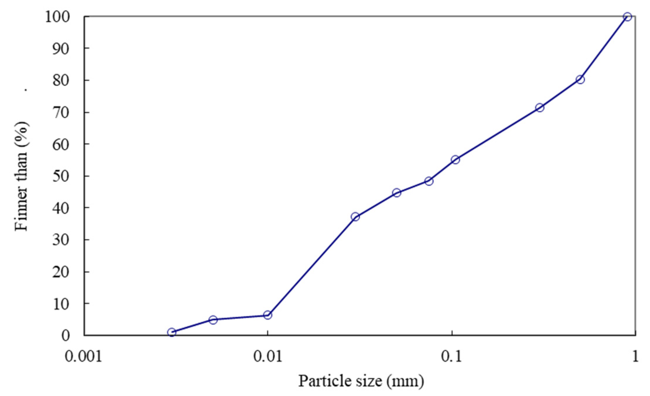
2.1. Materials
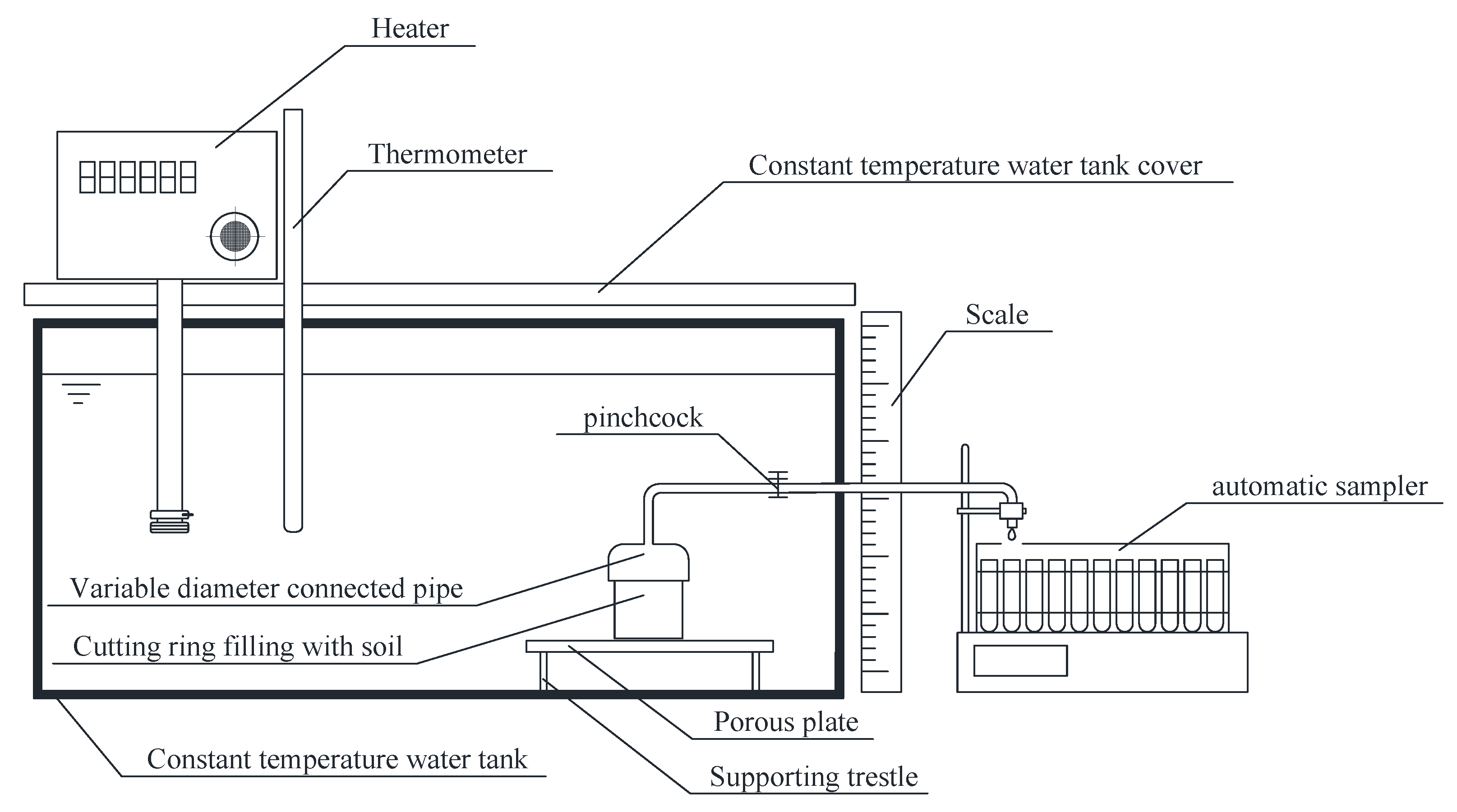
2.2. Experimental Methods
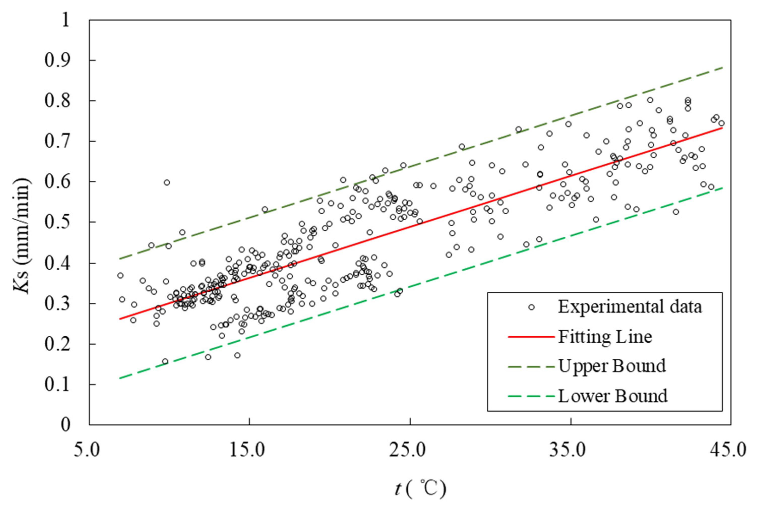
3. Results
4. Discussion
4.1. Comparison with Forest Standard of China
4.2. Comparison with Another Study Result
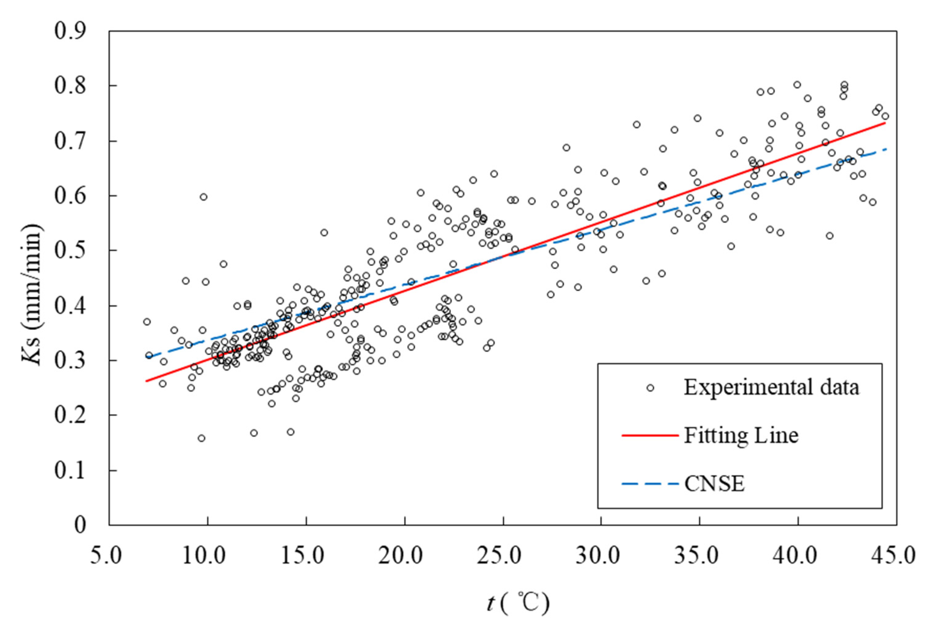
4.3. Formula Modification
5. Conclusions
Author Contributions
Funding
Institutional Review Board Statement
Informed Consent Statement
Data Availability Statement
Conflicts of Interest
References
- Mohanty, B.P.; Kanwar, R.S.; Everts, C.J. Comparison of saturated hydraulic conductivity measurement methods for a Glacial-Till soil. Soil Sci. Soc. Am. J. 1994, 58, 672–677. [Google Scholar] [CrossRef]
- Taiba, A.C.; Mahmoudi, Y.; Hazout, L.; Belkhatir, M.; Baille, W. Evaluation of hydraulic conductivity through particle shape and packing density characteristics of sand-silt mixtures. Mar. Georesour. Geotec. 2019, 37, 1175–1187. [Google Scholar] [CrossRef]
- Ye, W.; Wan, M.; Chen, B.; Chen, Y.; Cui, Y.; Wang, J. Effect of temperature on soil-water characteristics and hysteresis of compacted Gaomiaozi bentonite. J. Cent. South Univ. Technol. 2009, 16, 821–826. [Google Scholar] [CrossRef]
- Constantz, J.; Stonestrom, D.; Stewart, A.E.; Niswonger, R.; Smith, T.R. Analysis of streambed temperatures in ephemeral channels to determine streamflow frequency and duration. Water Resour. Res. 2001, 37, 317–328. [Google Scholar] [CrossRef]
- Jaynes, D.B. Temperature-variations effect on field-measured infiltration. Soil Sci. Soc. Am. J. 1990, 54, 305–312. [Google Scholar] [CrossRef]
- Cooper, C.A.; Thomas, J.M.; Lyles, B.F.; Reeves, D.M.; Pohll, G.M.; Parashar, R. A preliminary geochemical description of the geothermal reservoir at Astor Pass, Northern Pyramid Lake, Nevada. Geotherm. Resour. Counc. Trans. 2012, 36, 37–40. [Google Scholar]
- Ayenew, T.; Demlie, M.; Wohnlich, S. Application of numerical modeling for groundwater flow system analysis in the akaki catchment, central ethiopia. Math. Geosci. 2008, 40, 887–906. [Google Scholar] [CrossRef]
- Gedeon, M.; Mallants, D. Sensitivity analysis of a combined groundwater flow and solute transport model using Local-Grid refinement: A case study. Math. Geosci. 2012, 44, 881–899. [Google Scholar] [CrossRef]
- Zhang, F.; Zhang, Y.; Zhang, J. Temperature effect on soil water retention. Acta Pedol. Sin. 1997, 34, 160–169. [Google Scholar]
- Cho, W.J.; Lee, J.O.; Chun, K.S. The temperature effects on hydraulic conductivity of compacted bentonite. Appl. Clay Sci. 1999, 14, 47–58. [Google Scholar] [CrossRef]
- Cho, W.J.; Lee, J.O.; Kang, C.H. Influence of temperature elevation on the sealing performance of a potential buffer material for a high-level radioactive waste repository. Ann. Nucl. Energy 2000, 27, 1271–1284. [Google Scholar] [CrossRef]
- Fremond, M.; Nicolas, P. Macroscopic thermodynamics of porous media. Contin. Mech. Therm. 1990, 2, 119–139. [Google Scholar] [CrossRef]
- Zhang, F.C.; Zhang, R.D.; Kang, S.Z. Estimating temperature effects on water flow in variably saturated soils using activation energy. Soil Sci. Soc. Am. J. 2003, 67, 1327–1333. [Google Scholar] [CrossRef]
- Hopmans, J.W.; Dane, J.H. Temperature-Dependence of Soil-Water retention curves. Soil Sci. Soc. Am. J. 1986, 50, 562–567. [Google Scholar] [CrossRef]
- Gardner, W.R. Solutions of the flow equation for the drying of soils and other porous media. Soil Sci. Soc. Am. Proc. 1959, 23, 183–187. [Google Scholar] [CrossRef]
- Huang, Z.; Xu, H.; Bai, Y.; Yang, S. A Theoretical-empirical model to predict the saturated hydraulic conductivity of sand. Soil Sci. Soc. Am. J. 2019, 83, 64–77. [Google Scholar] [CrossRef]
- Ming, F.; Chen, L.; Li, D.; Wei, X. Estimation of hydraulic conductivity of saturated frozen soil from the soil freezing characteristic curve. Sci. Total Environ. 2020, 698, 134132. [Google Scholar] [CrossRef]
- Chen, L.; Li, D.; Ming, F.; Shi, X.; Chen, X. A fractal model of hydraulic conductivity for saturated frozen soil. Water 2019, 11, 369. [Google Scholar] [CrossRef] [Green Version]
- Delage, P.; Sultan, N.; Cui, Y.J. On the thermal consolidation of Boom clay. Can. Geotech. J. 2000, 37, 343–354. [Google Scholar] [CrossRef]
- Houston, S.L.; Lin, H.D. A thermal consolidation model for pelagic clays. Mar. Geotechnol. 1987, 7, 79–98. [Google Scholar] [CrossRef]
- Ikuo, T.; Pisit, K.; Ichiro, S.; Kanta, O. Volume change of clays induced by heating as observed in consolidation tests. Soils Found. 1993, 33, 170–183. [Google Scholar]
- Miller, C.J.; Yesiller, N.; Yaldo, K.; Merayyan, S. Impact of soil type and compaction conditions on soil water characteristic. J. Geotech. Geoenviron. 2002, 128, 733–742. [Google Scholar] [CrossRef]
- Vanapalli, S.K.; Fredlund, D.G.; Pufahl, D.E. The influence of soil structure and stress history on the soil-water characteristics of a compacted till. Geotechnique 1999, 49, 143–159. [Google Scholar] [CrossRef] [Green Version]
- Huo, L.; Qian, T.; Hao, J.; Liu, H.; Zhao, D. Effect of water content on strontium retardation factor and distribution coefficient in Chinese loess. J. Radiol. Prot. 2013, 33, 791. [Google Scholar] [CrossRef]
- Salager, S.; El Youssoufi, M.S.; Saix, C. Effect of temperature on water retention phenomena in deformable soils: Theoretical and experimental aspects. Eur. J. Soil Sci. 2010, 61, 97–107. [Google Scholar] [CrossRef]
- Huo, L.; Xie, W.; Qian, T.; Guan, X.; Zhao, D. Reductive immobilization of pertechnetate in soil and groundwater using synthetic pyrite nanoparticles. Chemosphere 2017, 174, 456–465. [Google Scholar] [CrossRef]
- Li, M.; Cao, X.; Liu, D.; Fu, Q.; Li, T.; Shang, R. Sustainable management of agricultural water and land resources under changing climate and socio-economic conditions: A multi-dimensional optimization approach. Agric. Water Manag. 2022, 259, 107235. [Google Scholar] [CrossRef]
- Yang, G.; Li, M.; Guo, P. Monte Carlo-based agricultural water management under uncertainty: A case study of Shijin irrigation district, China. J. Environ. Inf. 2022, 39, 152–164. [Google Scholar] [CrossRef]
- Huo, L.; Qian, T.; Hao, J.; Zhao, D. Sorption and retardation of strontium in saturated Chinese loess: Experimental results and model analysis. J. Environ. Radioact. 2013, 116, 19–27. [Google Scholar] [CrossRef]
- Cernicchiaro, G.; Barmak, R.; Teixeira, W.G. Digital interface device for field soil hydraulic conductivity measurement. J. Hydrol. 2019, 576, 58–64. [Google Scholar] [CrossRef]
- State Forestry Administration of China. Environmental Monitoring Method Standards-Soil Environment and Solid Waste, LY/T 1218-1999, 1st ed.; Chinese Standard Press: Beijing, China, 1999; p. 3.
- Ren, R.; Ma, J.; Sun, X.; Guo, X.; Zhang, K.; Fei, X. Experimental study on influence of system temperature and soil volume mass on saturated hydraulic conductivity under water-storage pit irrigation. Water Sav. Irrig. 2014, 3, 5–8. [Google Scholar]


| Parameter | Significance | Unit |
|---|---|---|
| Ks | Soil saturated hydraulic conductivity | mm/min |
| Kt | Soil saturated hydraulic conductivity at t °C | mm/min |
| K10 | Soil saturated hydraulic conductivity at 10 °C | mm/min |
| t | Soil water temperature | °C |
| D | Bulk density | g/cm3 |
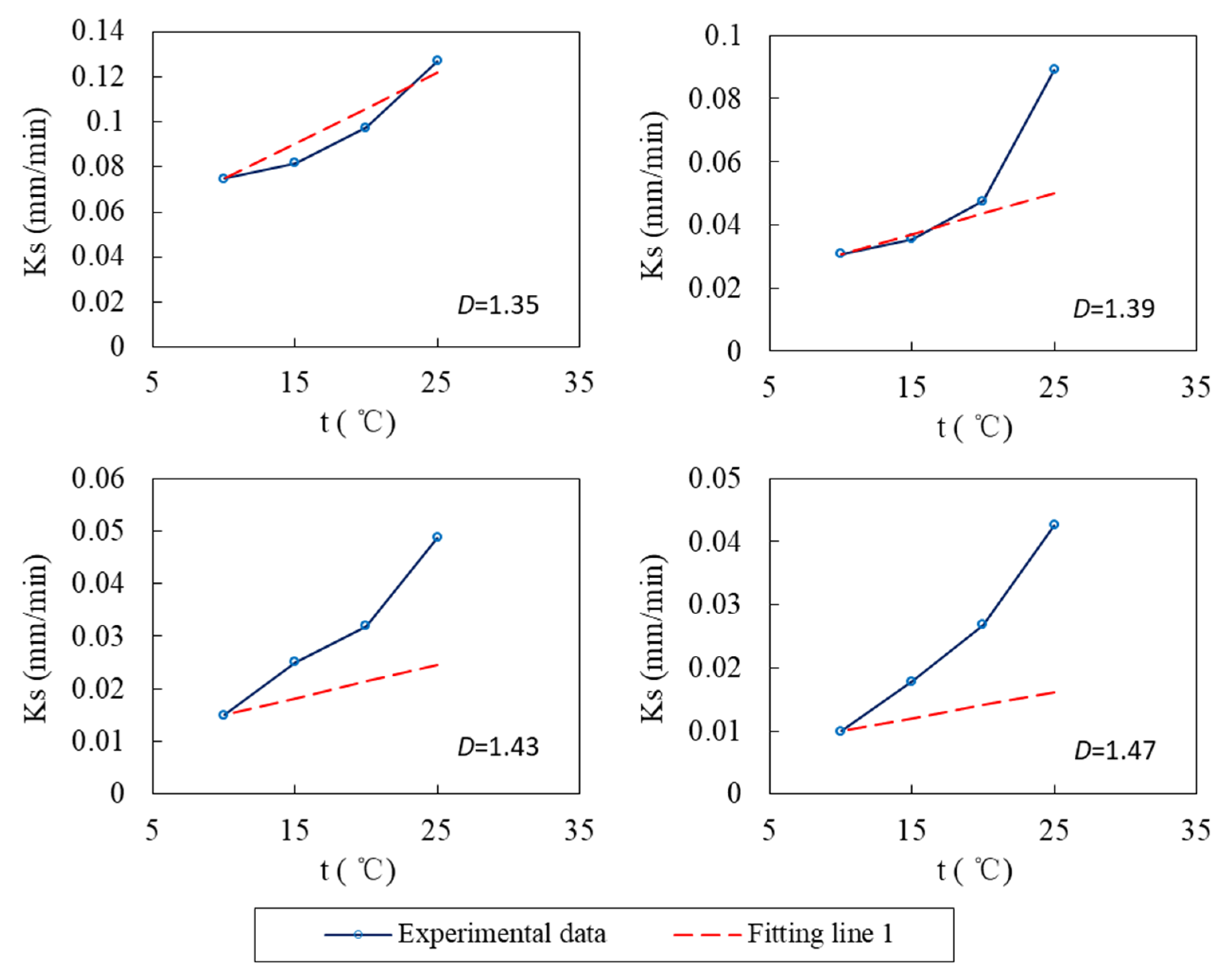
| D (g/cm3) | Fitting Line 1 | K10 (mm/min) | RMSE |
|---|---|---|---|
| 1.35 | Ks = 0.0435 + 0.0031 t | 0.0748 | 0.0095 |
| 1.39 | Ks = 0.0179 + 0.0013 t | 0.0307 | 0.0226 |
| 1.43 | Ks = 0.0088 + 0.0006 t | 0.0151 | 0.0153 |
| 1.47 | Ks = 0.0058 + 0.0004 t | 0.0100 | 0.0160 |
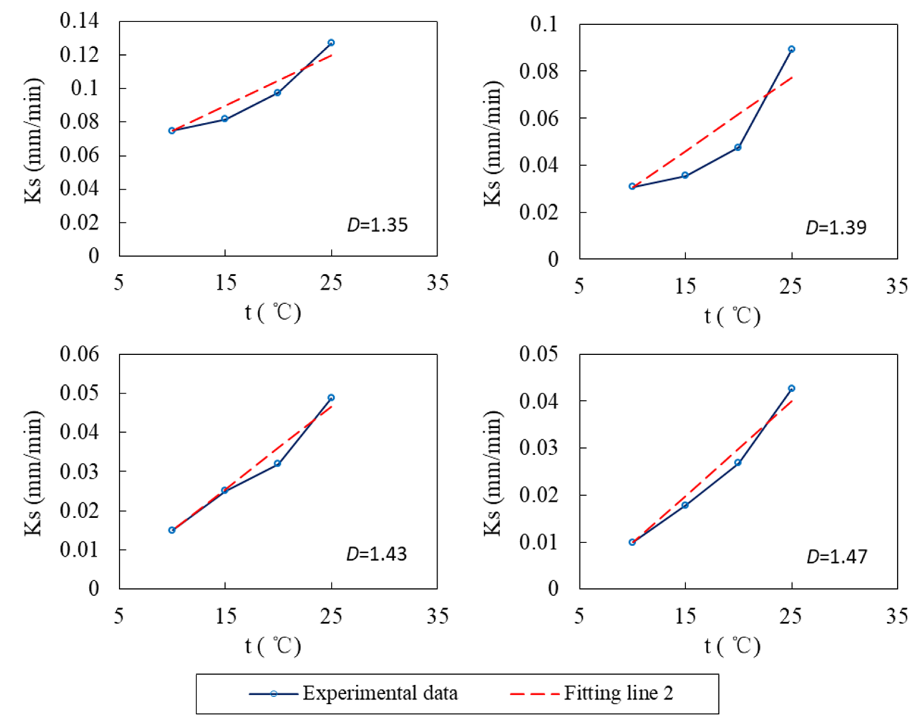
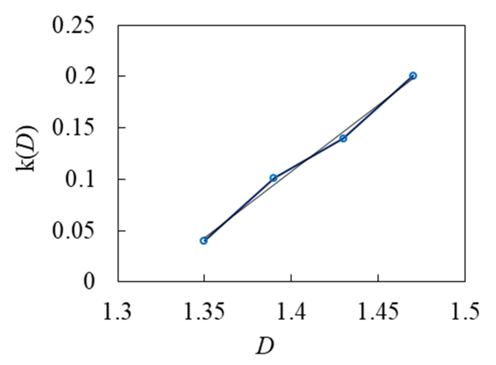
| D (g/cm3) | Fitting Line 2 | K10 (mm/min) | k(D) | RMSE |
|---|---|---|---|---|
| 1.35 | Ks = 0.0448 + 0.0030 t | 0.0748 | 0.0401 | 0.0065 |
| 1.39 | Ks = −0.0003 + 0.0031 t | 0.0307 | 0.1010 | 0.0107 |
| 1.43 | Ks = −0.0059 + 0.0021 t | 0.0151 | 0.1393 | 0.0024 |
| 1.47 | Ks = −0.0100 + 0.0020 t | 0.0100 | 0.2008 | 0.0023 |
Publisher’s Note: MDPI stays neutral with regard to jurisdictional claims in published maps and institutional affiliations. |
© 2022 by the authors. Licensee MDPI, Basel, Switzerland. This article is an open access article distributed under the terms and conditions of the Creative Commons Attribution (CC BY) license (https://creativecommons.org/licenses/by/4.0/).
Share and Cite
Yang, G.; Xu, Y.; Huo, L.; Wang, H.; Guo, D. Analysis of Temperature Effect on Saturated Hydraulic Conductivity of the Chinese Loess. Water 2022, 14, 1327. https://doi.org/10.3390/w14091327
Yang G, Xu Y, Huo L, Wang H, Guo D. Analysis of Temperature Effect on Saturated Hydraulic Conductivity of the Chinese Loess. Water. 2022; 14(9):1327. https://doi.org/10.3390/w14091327
Chicago/Turabian StyleYang, Gaiqiang, Yunfei Xu, Lijuan Huo, He Wang, and Dongpeng Guo. 2022. "Analysis of Temperature Effect on Saturated Hydraulic Conductivity of the Chinese Loess" Water 14, no. 9: 1327. https://doi.org/10.3390/w14091327
APA StyleYang, G., Xu, Y., Huo, L., Wang, H., & Guo, D. (2022). Analysis of Temperature Effect on Saturated Hydraulic Conductivity of the Chinese Loess. Water, 14(9), 1327. https://doi.org/10.3390/w14091327