Deep Learning for Streamflow Regionalization for Ungauged Basins: Application of Long-Short-Term-Memory Cells in Semiarid Regions

Abstract

Rainfall-runoff modeling in ungauged basins continues to be a great hydrological research challenge. A novel approach is the Long-Short-Term-Memory neural network (LSTM) from the Deep Learning toolbox, which few works have addressed its use for rainfall-runoff regionalization. This work aims to discuss the application of LSTM as a regional method against traditional neural network (FFNN) and conceptual models in a practical framework with adverse conditions: reduced data availability, shallow soil catchments with semiarid climate, and monthly time step. For this, the watersheds chosen were located on State of Ceará, Northeast Brazil. For streamflow regionalization, both LSTM and FFNN were better than the hydrological model used as benchmark, however, the FFNN were quite superior. The neural network methods also showed the ability to aggregate process understanding from different watersheds as the performance of the neural networks trained with the regionalization data were better with the neural networks trained for single catchments.

1. Introduction

In semiarid regions, long periods of water stress threat local populations and lead to economic losses [1], impair water quality [2], and consequently impact on local biodiversity [3]. In this scenario, efficient water resources planning and management (WRPM) are required to assure the sustainable development of the region. One strategy to provide information for WRPM is the use of rainfall-runoff models to simulate the hydrologic process in the basins, allowing to fill gaps in streamflow series and to project streamflow under different climate scenarios.

The basic structures for rainfall-runoff models are classified in (I) physically-based, (II) conceptual, and (III) empirical, according to the way they describe the natural hydrologic processes. Physically-based models rely on the physics to describe the mass and energy transfers in each cell of the basin, providing detailed information about the analyzed processes [4]. Consequently, this kind of model demands a large amount of data (e.g., boundary conditions and meteorological variables) and has high computational cost that restrains their application to lower dimension problems [5,6].

Conceptual or simplified physically-based rainfall-runoff models, in turn, make abstractions of the hydrologic processes. They simplify these processes, keeping the global dynamics, as the mass transfers between the different basin compartments, requiring a further understanding of the water movement in the hydrological cycle. A set of parameters which represents the average features in the catchment controls the mimicked dynamics in the conceptual models. Those parameters are calibrated to the targeted basin using the available rainfall and streamflow data [7]. Their simplified physics allows them to be applied with minimal data and computational costs at different scales [8].

Lastly, different from the other kinds of models, numerical rainfall-runoff models or fully data-driven approaches are not expected to describe the processes at a first moment. Instead, they are designed to find a numerical relation between the input data and the targeted streamflow output. In this kind of model, the comprehension of the modeled processes determines the input data selection. Data-driven models are also quite flexible and, although as any kind of model, their performance depends on the data availability, they require much less time for their development, allowing their application in real time and presenting efficient results for the streamflow prediction [9].

In general, the complexity of the process description in the model is limited by the data availability. In more complex models, the great number of inputs and parameters tends to result in uncertainty and inefficiency [10]. For these reasons, physically-based models have rarely practical use in data-scarce basins. However, even when conceptual or numerical models are used, a minimum of data is required for reliable streamflow estimation. Hence, streamflow simulation in ungauged basins (i.e., basins where we do not present satisfactory hydrological records) continues to be a great hydrological research challenge, since as pointed out by Sivapalan et al. [11], most basins fall under this definition.

In this aforementioned context, the International Association of Hydrological Sciences (IAHS) began the 2003–2012 decade with the elaboration of the initiative prediction in ungauged basins (PUB), which aims to formulate and implement appropriate programs to stimulate and raise awareness among the scientific community in a coordinated way, to achieve greater advances in this field [11]. The PUB is characterized by the extrapolation of information from gauged basins and, if possible, combined with the few data available of an ungauged basin, to allow the prediction of unknown or undocumented hydrological variables.

One strategy towards PUB is the regionalization of a conceptual model’s parameters, which allows to estimate the model parameters in ungauged basins through parameter values calibrated in gauged basins. Different types of regionalization techniques have been elaborated over the years and applied in different regions. Despite advances in the area, there is still no model superior to all the others, with performances varying for different regions and magnitudes [12,13,14]. At present, three types of flow regionalization are highlighted: regression-based [15,16], spatial proximity [17,18], and approach by physical proximity [17,19]. In regionalization, as the number of parameters grows, the difficulty to train a model increases, thus increasing the level of uncertainty, as the process they represent and the variables used become more conceptual and may not be physically relevant [20].

Using an appropriate framework, a data-driven approach can provide a regionalized rainfall-runoff model that simplifies the rainfall-runoff modeling and regionalization to a single step with the direct incorporation of proxy variables as input variables, having the flexibility to resemble a physical-based modeling (with the use of physical characteristics as a proxy variable) and benefiting a non-strict requirement of a complex set of physical input data. Several regression approaches, such as Multiple Regression [21], Stepwise [22], Artificial Neural Networks (ANN) [23,24,25], and Kernel-based approaches [26] are widely used in hydrological science with very robust results. In comparison to regression-based regionalization, the use of an ANN can possibly produce better results due to its ability to encompass both a linear and non-linear relationship between the proxy variables used and the streamflow series.

Recently, ANNs with sophisticated multilayer architectures have become famous with the name of Deep Learning (DL) due to their ability to solve complex computational problems [27]. To improve the ability of neural networks to learn time series, the Long-Short-Term Memory (LSTM) emerges as a State-of-Art ANN architecture that, different from the traditional Feedforward Neural Network (FFNN), is designed to learn time dependency information which is key in hydrological processes (e.g., for the storage in rainfall-runoff transformation) [28].

Few works have been done to address the application of LSTM to rainfall-runoff modeling. We highlight the works of Hu et al. [29], Xiang et al. [30], and Fan et al. [31] for individual catchments and Kratzert et al. [28] for streamflow regionalization. Hu et al. [29] and Xiang et al. [30] applied LSTM to predict hourly streamflow for flood estimation and compared its performance with widely used methods. The authors found that the LSTM models improved the accuracy of the predictions as they were superior to classical regression methods [30] and to FFNN model [29]. The results also show that the LSTM models are able to predict flood for catchments of different sizes and shapes. Fan et al. [31] compared the performance of LSTM models for daily rainfall-runoff modeling and found that the LSTMs performed better than FFNNs and the well-known SWAT model.

Kratzert et al. [28] applied LSTM to model daily streamflow in 291 catchments from the public CAMELS dataset [32] and found that the LSTMs, as individual catchment models, performed better mainly in snow-driven catchments and worse in arid basins as the long-term dependencies are more important for snow-driven processes (e.g., snow accumulation and snowmelt). The LSTM model also performed slightly better than the conceptual model used as a benchmark. As regional models, the researchers found that LSTM has competing performance against individual catchments models. However, no other regional model was used as a benchmark for comparison.

Kratzert et al. [28] is, up to now, the only work that discusses the application of LSTMs as regional models for ungagged basins. Although their results show that the performance of LSTM is better for snow-driven catchments where the long-term memory has a key role in the hydrological transformation, it is not clear if its application should be restrained to this case or if simpler ANN architectures would outperform them in situations where long-term memory is not a major factor.

The main purpose of this work is to discuss the application of LSTM as a streamflow regionalization method against traditional Feedforward ANN and conceptual models in a practical framework for the Brazilian semiarid conditions such as reduced data availability, high precipitation variability, shallow soil catchments, and intermittent rivers.

Specifically, our goal is to answer the following questions:

• Can the LSTM be used as a hydrological and/or streamflow regionalization model in a semiarid region? Does it outperform a conceptual hydrological model and the FFNN? How does their performance change with the amount of data in each catchment?
• Can simple alterations in FFNN be done to include short-term memory results in a model that outperforms the LSTM in hydrological modeling and streamflow regionalization in a semiarid region with shallow soils and intermittent rivers?

The questions in 1. are mainly related to the reduced data availability that may limit the application of both FFNN and LSTM due to their higher parameter number in comparison to conceptual hydrological models. The question in 2. arises from the short memory of the streamflow of the studied catchments due to the semiarid climate and shallow soil characteristics that cause the depletion of the soil storage during the dry season. In a short memory process, an FFNN with a simple alteration such as including streamflow lags as input variables may be more efficient (performance vs. number of parameters) than a deeper approach such as LSTM.

2. Materials and Methods

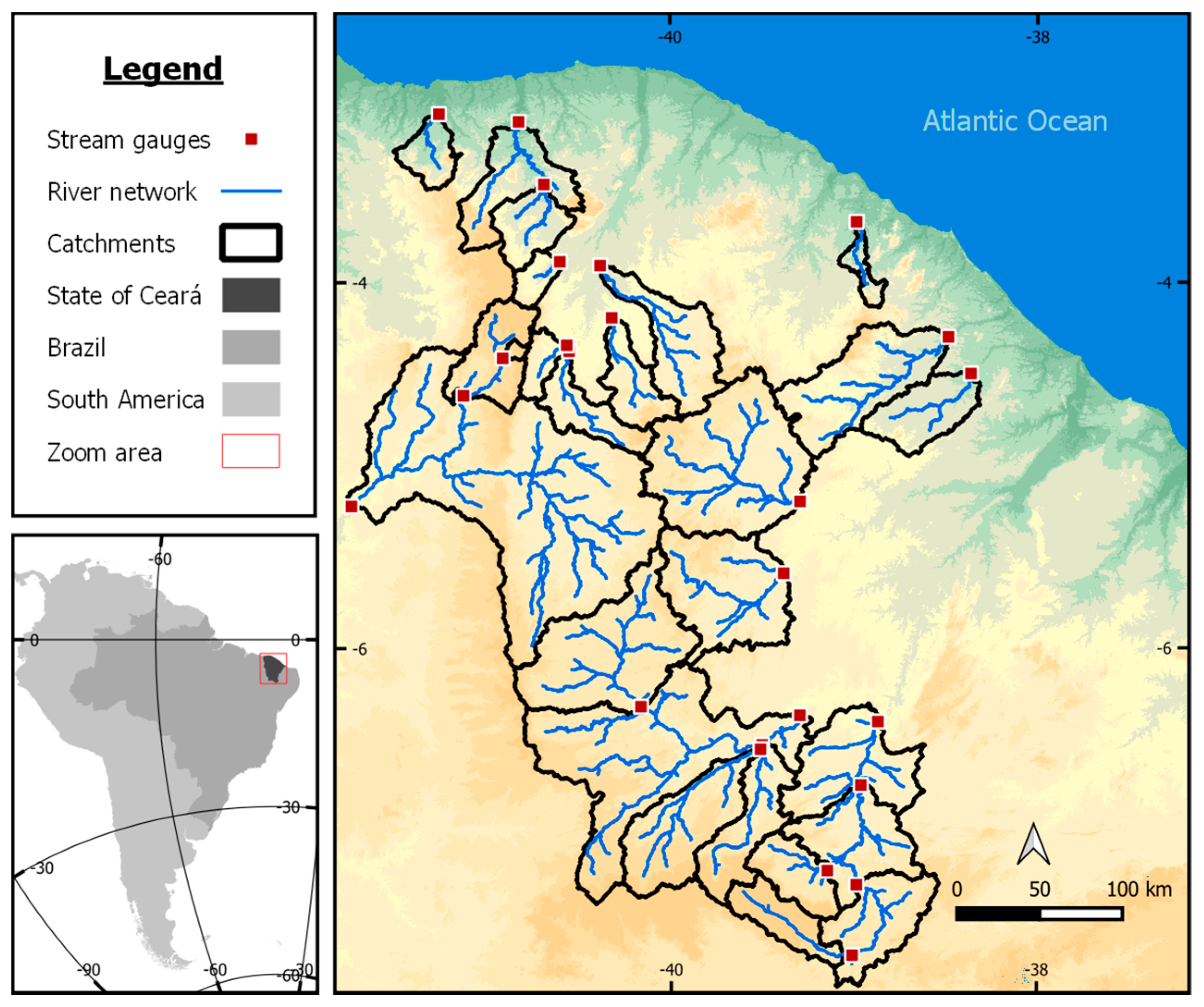
2.1. Case Study and Data

The proposed framework for PUB was applied to streamflow estimation in 25 basins in the semiarid region of the State of Ceará. The State of Ceará is located in the northeast of Brazil, its area is about 148,826 km² and a major part of the State is semiarid, which has the caatinga as the main native vegetation, a semiarid biome. The climate is predominantly semiarid, where most of the rainfall concentrates in 3 or 4 months, reaching less than 500 mm yearly in some regions. On the State coast, tropical weather predominates with an average annual rainfall around 1000 mm. In the humid and high mountains, the caatinga gives way, as the altitude rises, to the Atlantic Forest. Evapotranspiration, which is much more intense than in the Country Depression, ranges from 1000 mm to over 2000 mm annually. In these humid islands, temperatures also vary more than in the rest of the state: in colder months (particularly July), lows may reach below 15 °C, but in warmer months (notably December), temperatures can reach close to 35 °C. On the coast, the mangroves and typical coastal vegetation predominate. Even at very low altitudes, rainfall and humidity are higher than in the Country Depression. Daily average temperatures range from about 22 °C to 32 °C.

The plateaus and coasts bordering the territory of Ceará are sedimentary by formation, while the various mountain ranges found in the interior of the depression, particularly the distance from the coast, are ancient massifs of crystalline rock origin. The average coastal temperature is 24 °C to 28 °C. In the mountains, the temperature is 20 °C to 25 °C and in the Country Depression, the temperature is 26 °C to 29 °C. The state presents uniform geomorphological characteristics, almost 74% of the state has shallow soils with crystalline embasement, which results in low base flows and a reduced importance of the long-term memory of the storage process in the rainfall-runoff transformation.

Rainfall and streamflow data were collected in the HidroWeb/ANA database provided by the National Water Agency (ANA). Streamflow data were obtained from 25 stream gauges in the State of Ceará, selected from ANA dataset by avoiding gauges with large upstream dams, since they can significantly modify the natural flow regime. The observed streamflow time series are heterogeneous, and their range varies according to the beginning of each station data record, in which some stations have almost 100 years of record and less than 20 years in others. Figure 1 shows a general view of the area studied and the location of the stations.

It is expected that catchments with similar characteristics behave similarly, so it is important to pass these components into the regionalization models. All catchment characteristics used in this study can be found in

Table 1. Basins’ physical characteristics.

Stream-flow Station	Declivity—D (%)	Contribution Area of the Fluviometric Station—A (km2)	Total Drainage Length—CTD (km)	Drainage Density—DD (km−1)	Soil Water Storage Capacity (CAD) (mm)	Average Curve Number—CN (mm)	Basin Compact-ness Coefficient (Kc)—Kc	Portion of the Basin in the Crystalline Rock—Cr
34730000	0.069	897.372	528.790	0.589	59.483	56.774	1.990	0.000
34740000	0.065	2221.989	356.001	0.160	51.100	59.941	1.085	0.000
34750000	0.056	19,185.920	10,051.126	0.524	73.315	73.945	2.560	0.588
35050000	0.092	997.264	606.451	0.608	71.461	82.375	1.950	0.534
35125000	0.081	1501.237	1501.190	1.000	65.377	84.315	1.902	0.921
35170000	0.081	3967.244	3523.080	0.888	69.009	79.753	2.217	0.770
35210000	0.071	1566.680	1574.683	1.005	74.984	82.767	2.772	0.957
35223000	0.082	693.135	636.738	0.919	82.157	84.314	2.178	0.763
35240000	0.100	1532.777	1309.706	0.854	66.220	85.743	2.467	0.913
35260000	0.078	2875.183	2690.396	0.936	61.125	82.961	2.493	0.934
35263000	0.077	587.889	547.171	0.931	82.225	83.172	1.975	0.773
35668000	0.082	495.859	364.205	0.734	76.364	82.358	2.876	0.926
35880000	0.086	4085.575	3084.452	0.755	85.831	82.799	2.431	0.875
35950000	0.037	2027.716	1442.687	0.711	85.603	80.000	2.090	0.815
36020000	0.053	5852.006	4284.214	0.732	77.478	83.589	2.336	0.923
36125000	0.080	3533.321	2492.858	0.706	84.805	81.209	2.285	0.733
36130000	0.083	5996.827	3935.060	0.656	87.925	81.907	2.388	0.737
36160000	0.072	20,664.322	14,792.266	0.716	75.959	82.330	2.845	0.818
36210000	0.078	1665.995	1106.796	0.664	97.794	82.833	2.070	0.401
36220000	0.028	1564.877	355.644	0.227	88.639	84.871	2.588	0.153
36250000	0.055	4240.717	2596.731	0.612	80.005	80.765	2.680	0.457
36270000	0.070	8869.966	6943.068	0.783	77.104	81.294	2.118	0.605
36290000	0.067	12,381.522	9914.359	0.801	79.707	82.338	2.424	0.689
36470000	0.085	998.024	1332.280	1.335	66.302	78.687	2.102	0.988
36520000	0.080	7035.737	7678.188	1.091	65.151	85.408	2.169	0.978

The Declivity represents the Average Catchment Slope, and with the Drainage density (DD) and the compactness coefficient (Kc) express the water transport in the catchment. The Contribution area of the fluviometric station (A) and the Total drainage length (CTD) may provide the information about the volume of water in the Catchment. Values of Portion of the basin in the crystalline bedrock (Cr) and Average Curve Number (CN) can represent the soil storage capacity and infiltration-runoff relationships.

and have been published [33].

2.2. Methodology

This section represents the methodology used in this work and it is organized in four parts. In the first section, the models used for the rainfall-runoff modeling and streamflow regionalization are described: (i) Soil Moisture Account Modeling (SMAP) which is the benchmark conceptual model, (ii) the traditional Feedforward Neural Network (FFNN) and (iii) the Long-Short-Term Memory neural network (LSTM). The second part describes the feature selection procedure used for the ANN regional models. The third part describes the design of the experiments that will base the results and discussions. The fourth part describes the performance evaluation metrics used in the analysis of the models. All models analyzed and described in this article calculate flow with monthly time step.

In this study, we propose the application of two different ANN architectures, a Feedforward Neural Network (FFNN) and a Long-Short-Term Memory (LSTM), both regionalized in one single step. The difference between the two approaches lies in how the monthly dependency is incorporated. LSTM by construction is a recurrent neural network (RNN), incorporating explicit time dependency. In contrast, time dependency in FFNNs can be only implicitly incorporated by including streamflow and rainfall lags as proxy variables. All ANN were written using Python’s framework TensorFlow 2.0 [34].

2.3. Rainfall Runoff and Streamflow Regionalization Models

2.3.1. Soil Moisture Account Modeling (SMAP)

Soil Moisture Accounting Procedure (SMAP) [35] is a lumped conceptual model that is widely used by water resources agencies in Brazil [33,36]. SMAP, in its monthly version, tries to represent the storage and water mass balance in the basin through two fictional linear reservoirs (subsurface and ground water) and uses observations of the catchment’s average precipitation and evapotranspiration as inputs.

For each Precipitation event (P), a mass balance is made. There are 4 major parameters that must be calibrated: Soil Saturation Capacity (SAT), superficial runoff rate (PES), the recharge coefficient of the aquifer (CREC), and the depletion rate (Kkt) of the water reservoir (RSub). For basins located in the State of Ceará, only two (SAT and PES) of these parameters are useful for hydrological analysis as the shallow soils result in CREC = 0 and makes the output of the model to be without sensitivity for Kkt [37]. Other studies used SMAP in Ceará catchments [38,39] and in Brazil [40,41].

Barros et al. [33] used SMAP to calculate SAT and PES for the same catchments used in this study. Once with the calibrated parameters, they used physiographical characteristics of the basins to generate a linear equation for the regionalization of the SAT and PES parameters by three different Multiple Linear Regression approaches. The regression methods used were: (I) Generalized Linear Model (GLM) using a normal distribution to estimate the coefficients of physical-climatic variable; (II) GLM similar to (I) but using a gamma distribution, and (III) Robust Regression. They found that the best linear equations for the regionalization of the model in the State would be:

$$\mathrm{SAT}=3021.6-2026.74\times \mathrm{Cr}$$

(1)

$$\mathrm{PES}=5.405742+42.286774\times \mathrm{D} -3.803776\times \mathrm{DD} -2.51601\times \mathrm{Cr}$$

(2)

where Cr is the portion of the basin over the crystalline bedrock (%), D is the basin mean declivity (%), DD is the drainage density (km⁻¹).

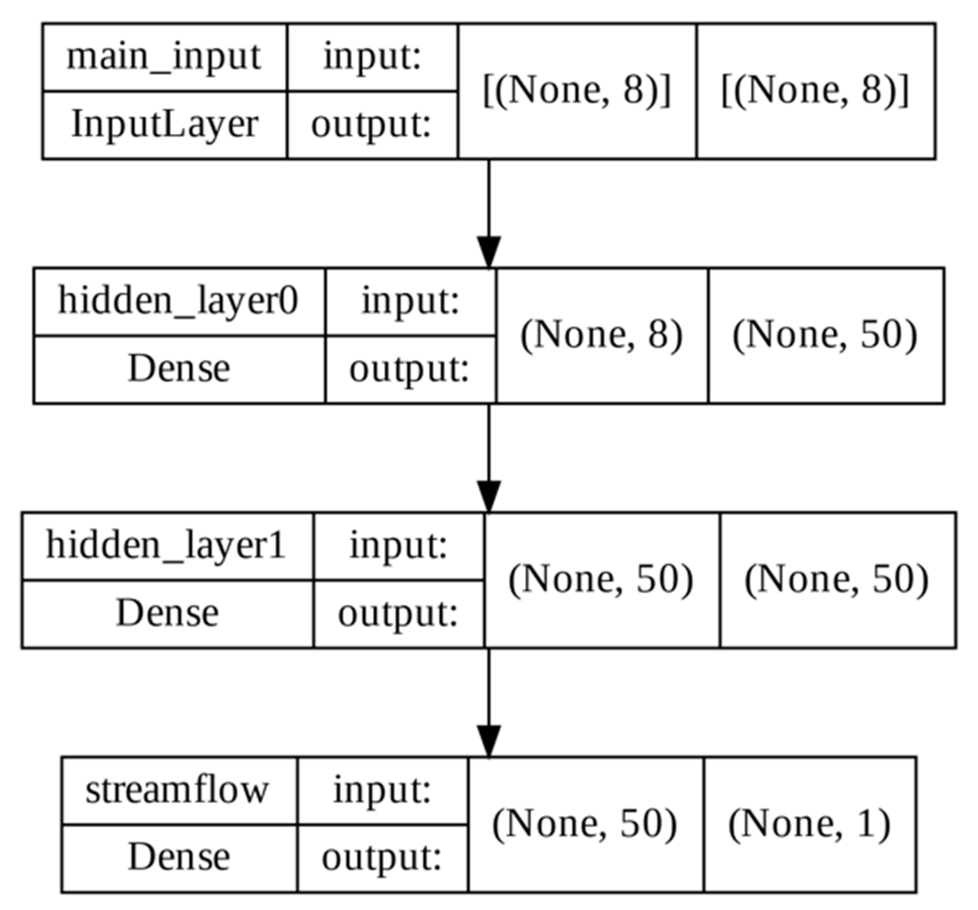
2.3.2. Feedforward Neural Network (FFNN)

Although ANNs’ basis was formulated by McCulloch and Pitts in 1943 [42], its use was only possible in the mid-1980s and 1990s with the increase of the processing power of computers and the availability of data. Its conceptualization is based on the elaboration of an algorithm that tries to mimic the functioning of the human neuron. Haykin [43] defines a neural network as a massively distributed processor in parallel that has a natural propensity for storing knowledge and making it available for use. It resembles the brain in two aspects: knowledge is acquired by the network through a learning process and the forces of the interneural connection, known as synaptic weights, are used to store knowledge. According with “universal approximation theorem” a neural network of one layer can approximate any linear function; a two layers network, with the necessary number of hidden neurons, can approximate any continuous function, and with three or more layers, it can approximate any function, including discontinuous, respecting the range of Inputs and Outputs [43]. However, it should be noted that the choice for deep networks is not always necessarily better because larger networks often lead to overfitting and have higher computational cost, justifying the choice for a simpler architecture.

Each layer has a set of nodes (neurons), nodes from one layer are fully connected to the nodes of the next through a vector of weights, and the final layer is the output known as output layer. The general form of a Feedforward Neural Network can be expressed as:

$$\mathrm{y} = \mathrm{f}\left({\displaystyle \sum }_{\mathrm{i}=1}^{\mathrm{n}}{\mathrm{x}}_{\mathrm{i}}{\mathrm{w}}_{\mathrm{i}}+{\mathrm{b}}_{\mathrm{i}} \right)$$

(3)

where $\mathrm{y}$ is the output of a node, $\mathrm{f}$ is the activation function, and ${\mathrm{x}}_{\mathrm{i}}$, ${\mathrm{w}}_{\mathrm{i}}$ and ${\mathrm{b}}_{\mathrm{i}}$ are the input, weights, and bias vectors, respectively. The role of an activate function is to decide if a neuron’s input contains relevant information for the prediction or not and to add non-linearity to the neural network.

The activation function of the hidden layers used was rectified linear unit (ReLU), since it is scale-invariant and computational efficient, as it only compares, adds, and multiplies and has fewer vanishing gradient problems if compared with other major activation functions, such as sigmoid and tanh.

$$\mathrm{f}\left(\mathrm{x}\right)={\mathrm{x}}^{+}= \max \left(0,\mathrm{x}\right)$$

(4)

The flux of information in a neural network is divided in two phases: the first is the Feedforward, where the input is processed from the layer-to-layer until the output layer and a backpropagation phase, where the error (i.e., the difference of predicted and measured values) is discounted of the synaptic weights of every node thrown at the gradient descendent algorithm.

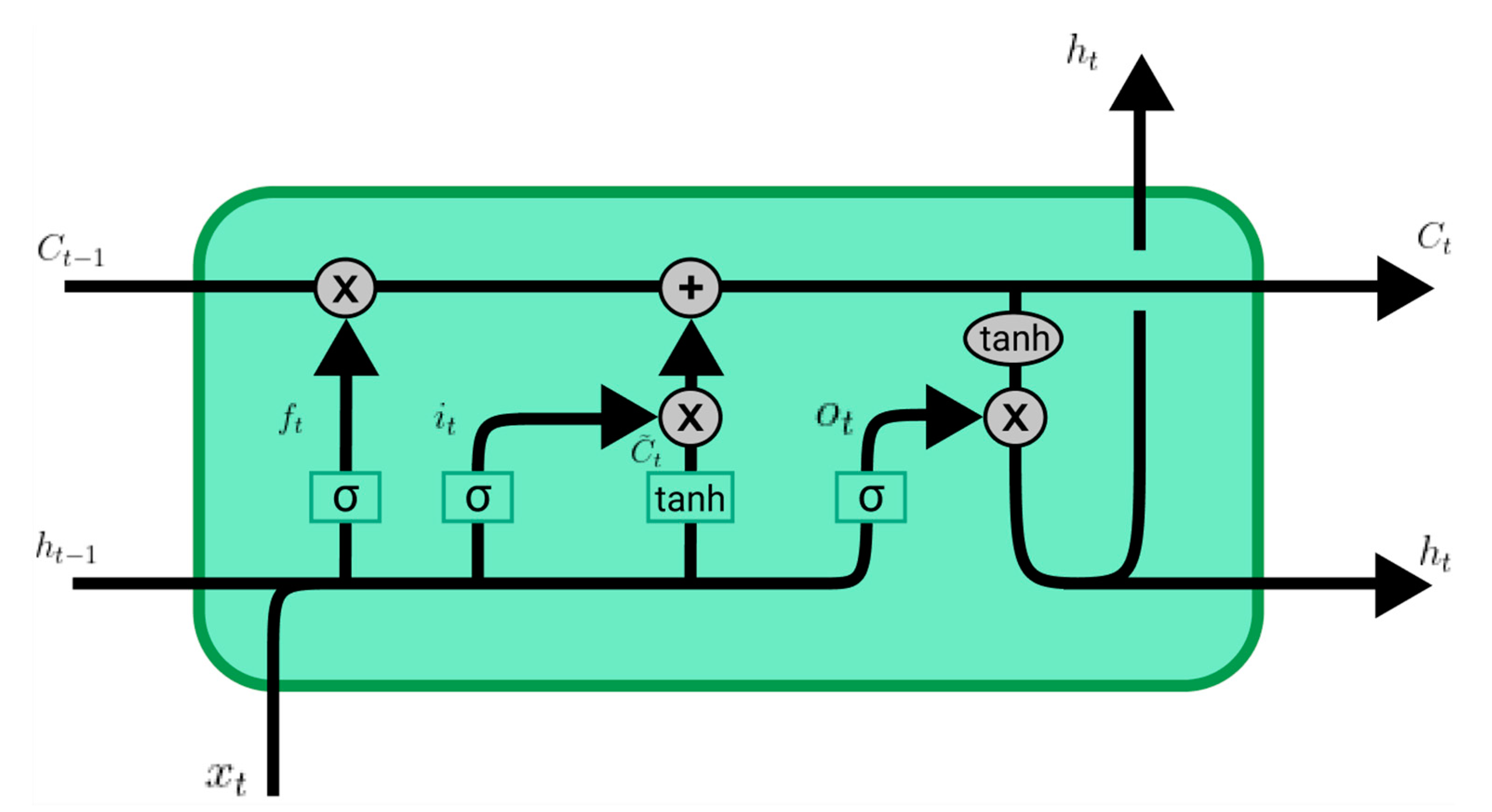
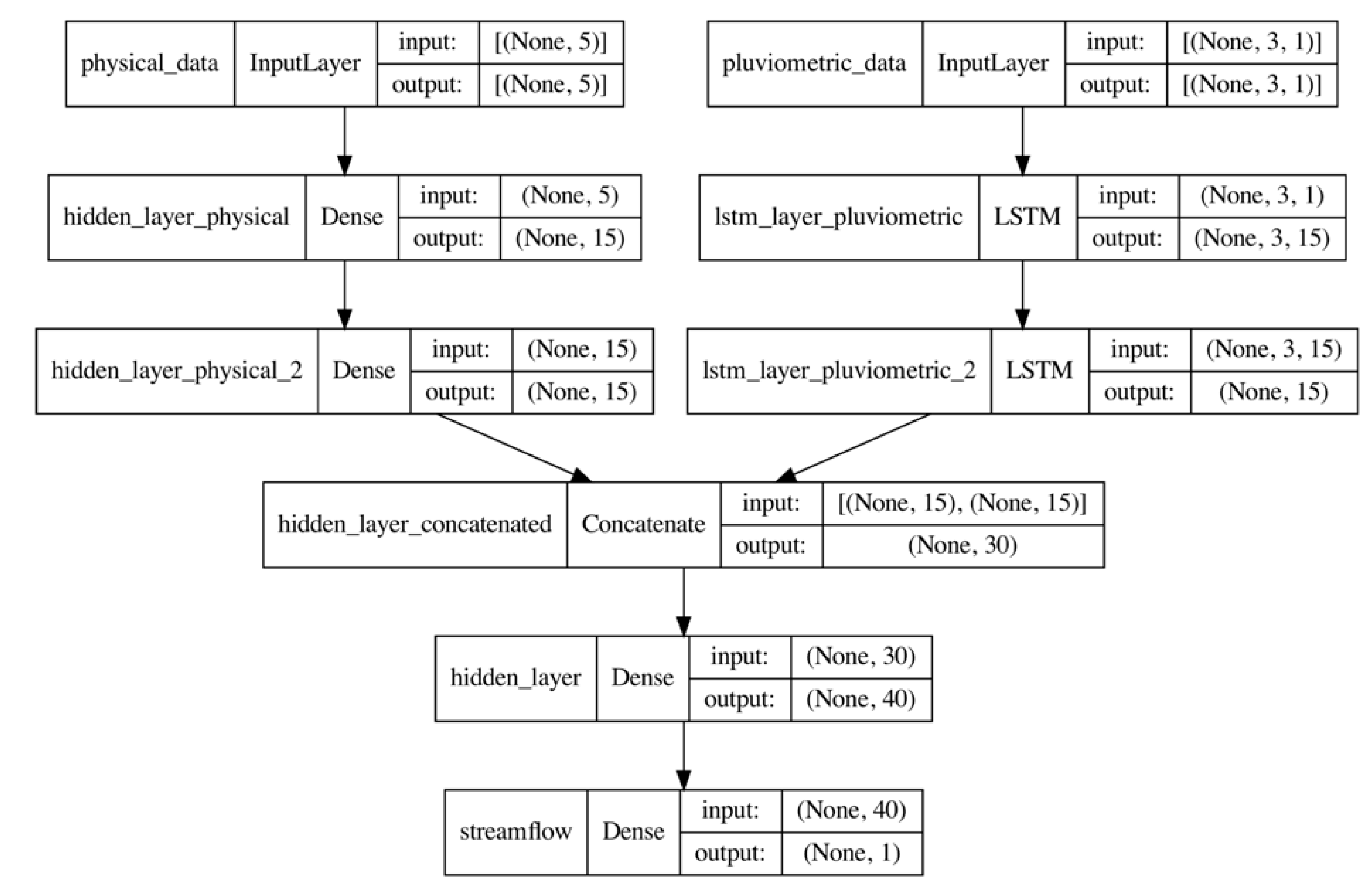
2.3.3. Long-Short-Term Memory Neural Network (LSTM)

This type of network was first introduced by Ref. [44] and was designed for sequence dependent problems, once their application became popular not only for time dependency modeling, but also for image captioning, language modeling, translation, and speech recognition.

The LSTM neural network’s main characteristic is their Long-Term Memory, that allows the network to “remember” important information for a long time when compared to simple Recurrent Neural Networks (RNN). These are also known as Elman’s Networks [45], which are subject to the vanishing Gradient Problem [46] by not being able to store lagged information through long periods of time; usually Elman’s networks do not save information for more than 10 steps. The capacity of storying Long-Term Memory is due to its internal state that, for each time step, calculates the output and contains weight parameters for it as well as for the input. The Memory Cell contains gates which are weighted functions that handle the flow of information into and out of the cell.

2.3.4. LSTM Model Explanation

Figure 2 is a graphical representation of the mathematical operations present in an LSTM Cell. Given an input vector $\mathrm{x}=\left[{\mathrm{x}}_1,{ \mathrm{x}}_2,\dots ,{\mathrm{x}}_{\mathrm{n}}\right]$, “n” being the consecutive time steps of an independent variable (in this study, we use precipitation data). The model processes the data sequentially and for a step t ($1 \le \mathrm{t} \le \mathrm{n}$), the input ${\mathrm{x}}_{\mathrm{t}}$ produces an output ${\mathrm{h}}_{\mathrm{t}}$. The model “decides” which it “saves” or “discards” information through its “gates”. In a LSTM Cell, there are three gates: the forget gate (${\mathrm{f}}_{\mathrm{t}}$), the input gate (${\mathrm{i}}_{\mathrm{t}}$), and the output gate (${\mathrm{o}}_{\mathrm{t}}$).

The forget gate concatenates the input vector ${\mathrm{x}}_{\mathrm{t}}$ and the previous output ${\mathrm{h}}_{\mathrm{t}-1}$, and defines which information is removed from the memory (cell state). ${\mathrm{W}}_{\mathrm{f}}$ and ${\mathrm{b}}_{\mathrm{f}}$ are tensors of learnable parameters. Then, a sigmoid function is applied returning a tensor of numbers between 0 and 1 that multiplies the previous cell state ${\mathrm{C}}_{\mathrm{t}-1}$. If a value outputs 0, it will be completely forgotten and if its value is 1, it will be entirely kept. In the first step, the hidden state ${\mathrm{h}}_{\mathrm{t}-1}$ is initialized by a vector of zeros with the same length of the series.

$${\mathrm{f}}_{\mathrm{t}}=\mathsf{\sigma }\left({\mathrm{W}}_{\mathrm{f}}\cdot \left[{\mathrm{h}}_{\mathrm{t}-1},{\mathrm{x}}_{\mathrm{t}}\right]+{\mathrm{b}}_{\mathrm{f}}\right)$$

(5)

Then, the next gate decides if either a value is updated (added) or not to the cell state, by multiplying it by a sigmoid and a tanh (hyperbolic tangent) function, creating the vector ${\tilde{\mathrm{C}}}_{\mathrm{t}}$ with values to be added to the state. After that, both vectors are multiplied and added to the previous cell state. Therefore, ${\mathrm{i}}_{\mathrm{t}}$ is a vector in the range (0, 1) and ${\tilde{\mathrm{C}}}_{\mathrm{t}}$ is a vector in the range (−1, 1), and ${\mathrm{W}}_{\mathrm{i}}$, ${\mathrm{b}}_{\mathrm{i}}$, ${\mathrm{W}}_{\mathrm{c}}$ and ${\mathrm{b}}_{\mathrm{c}}$ are a set of learnable parameters:

$${\mathrm{i}}_{\mathrm{t}}=\mathsf{\sigma }\left({\mathrm{W}}_{\mathrm{i}}\cdot \left[{\mathrm{h}}_{\mathrm{t}-1},{\mathrm{x}}_{\mathrm{t}}\right]+{\mathrm{b}}_{\mathrm{i}}\right)$$

(6)

$${\tilde{\mathrm{C}}}_{\mathrm{t}}=\tan \mathrm{h}\left({\mathrm{W}}_{\mathrm{c}}\cdot \left[{\mathrm{h}}_{\mathrm{t}-1},{\mathrm{x}}_{\mathrm{t}}\right]+{\mathrm{b}}_{\mathrm{c}}\right)$$

(7)

The updated cell state can be calculated with the previous results:

$${\mathrm{C}}_{\mathrm{t}}={\mathrm{f}}_{\mathrm{t}}\times {\mathrm{C}}_{\mathrm{t}-1}+{\mathrm{i}}_{\mathrm{t}}\times {\tilde{\mathrm{C}}}_{\mathrm{t}}$$

(8)

To calculate the output of the cell (i.e., hidden state), the new cell state passes through tanh to its values which fit between −1 and 1, and is multiplied by the output of the output gate (${\mathrm{O}}_{\mathrm{t}}$), being ${\mathrm{W}}_{\mathrm{o}}$ and ${\mathrm{b}}_{\mathrm{o}}$, a set of learnable parameters. This gate defines which information of the cell state is used as output.

$${\mathrm{o}}_{\mathrm{t}}=\mathsf{\sigma }\left({\mathrm{W}}_{\mathrm{o}}\cdot \left[{\mathrm{h}}_{\mathrm{t}-1},{\mathrm{x}}_{\mathrm{t}}\right]+{\mathrm{b}}_{\mathrm{o}}\right)$$

(9)

$${\mathrm{h}}_{\mathrm{t}}={\mathrm{o}}_{\mathrm{t}}\cdot \tan \mathrm{h}\left({\mathrm{C}}_{\mathrm{t}}\right)$$

(10)

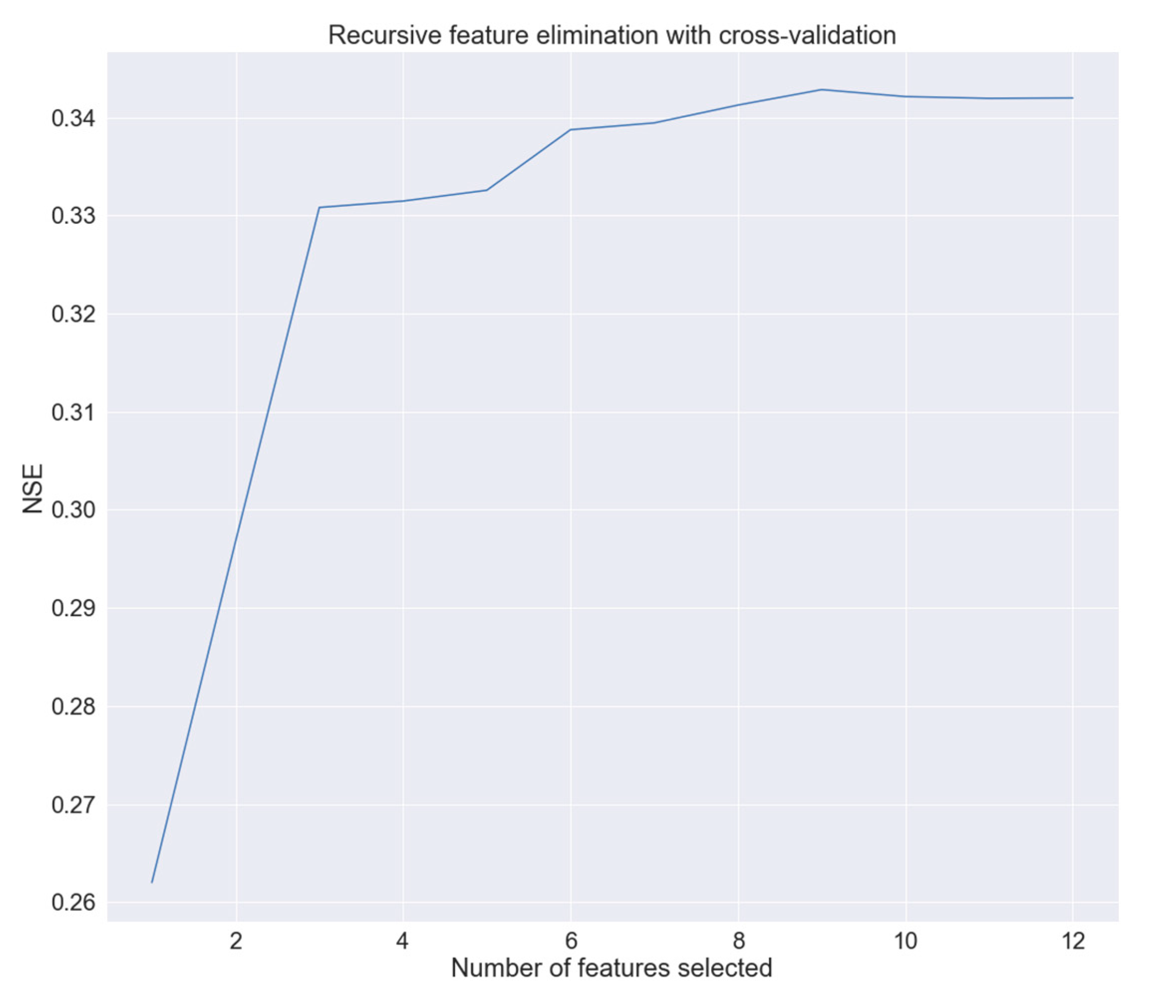
2.4. Feature Selection for the Streamflow Regionalization Models

The features were selected by Recursive Feature Elimination (RFE) [47] with cross-validation (RFECV) using a linear rainfall-runoff model that is fitted by minimizing a regularized empirical loss with Stochastic Gradient Descent (SGD). The RFE reduces the number of features by building a model with the entire set of features and computes the importance score for each feature (e.g., the coefficients of a Linear Model), then it eliminates the least important attribute. This procedure is repeated recursively on the pruned set until the desired number of features is reached. The RFECV consists of an RFE that uses a cross-validation loop to find the optimal number of features.

2.5. Experimental Design

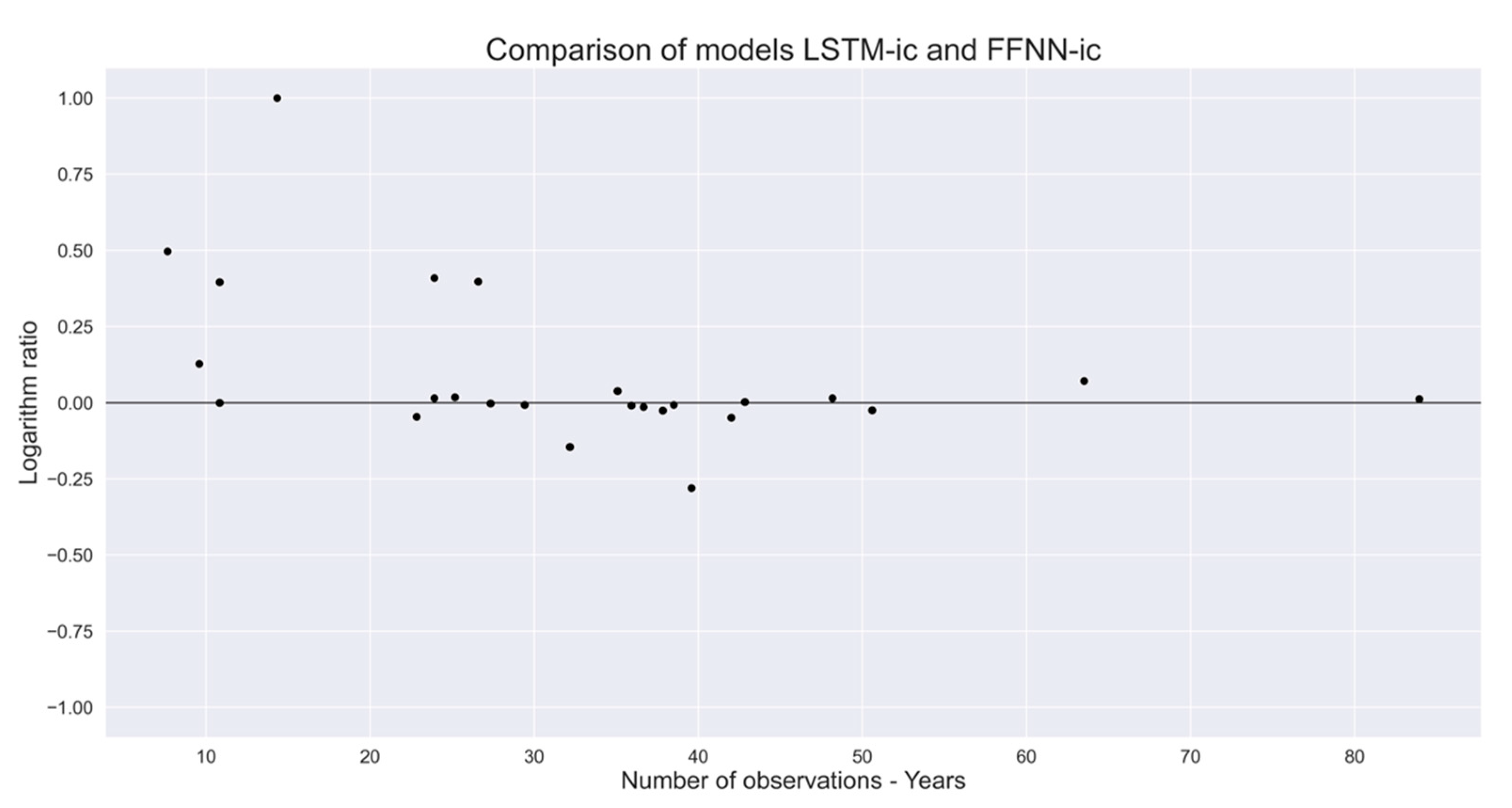
2.5.1. Experiment 1: LSTM and FFNN as Rainfall-Runoff Models

The first experiment seeks to evaluate the general skill of the LSTM and FFNN to model the monthly rainfall-runoff processes in each of the studied catchments. One LSTM network and one FFNN network are trained separately for each catchment. The Feedforward model received inputs the previous six months of Precipitation (mm), while LSTM model received three months; once its performance with three months was superior to its performance with six. The FFNN used 2 hidden layers with 30 neurons each and the recurrent model used two LSTM layers with 15 neurons and one Dense Layer with 25 neurons.

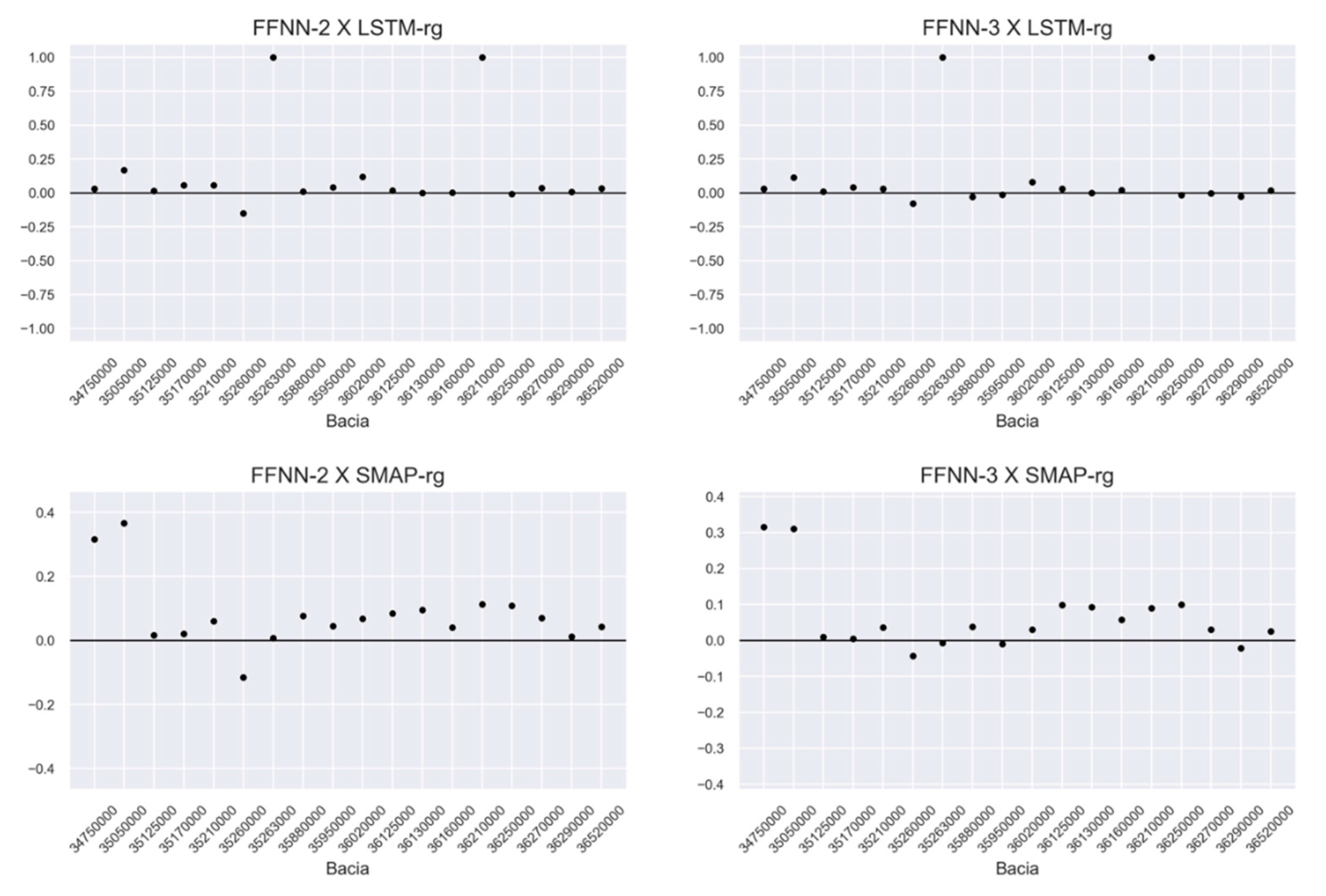
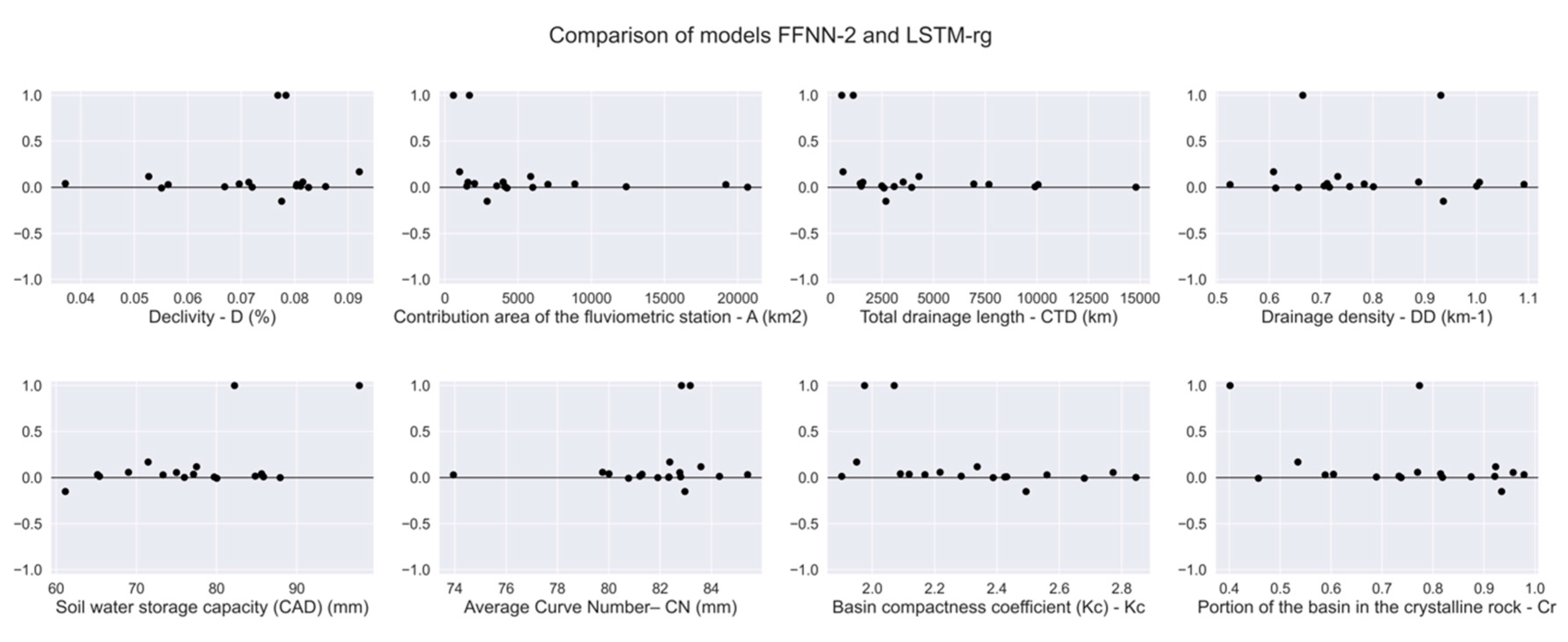
2.5.2. Experiment 2: LSTM and FFNN as Streamflow Regionalization Models for Ungauged Basins

The second experiment investigates the capability of LSTMs for regional modeling. Three regional models were elaborated: FFNN-2, FFNN-3, and LSTM-rg. The differences between all FFNN models are shown in the set of inputs in

Table 2. Representation of models’ inputs.

Experiment	Model	D	CT	A	P	CTD	DD	CAD	CN	Kc	Cr	E	Precipitation Lags	Streamflow Lags
1	FFNN-ic
	LSTM-ic
	SMAP-ic
2	FFNN-2
	FFNN-3
	LSTM-rg
	SMAP

* Green cells indicate the presence of a given attribute in the model and red cells indicate the absence.

. The inputs for FFNN-3 and LSTM-rg are the same.

As inputs, all 3 models require three previous months of precipitation as meteorological inputs and catchment area (A), total drainage length (CTD), average Curve Number (CN), and portion of the basin in the crystalline bedrock (Cr) as physical inputs. Model FFNN-2 also require two previous months of streamflow. The inputs of each of the regional models are presented in Table 2.

For the network design, both FFNN models used 2 hidden layers with 50 neurons each. Since LSTM cells only read a series of data, it is not recommended to pass the physical data into it, so it was passed into two Feedforward layers, also known as Dense Layers, with 15 neurons each, and the pluviometric lag of the 3 previous months into two LSTM layers with 15 neurons each. Then, those 2 layers were concatenated and passed through another Dense Layer with 40 neurons. For all Dense layers, ReLU was used as an activation function. Figure 3 and Figure 4 represent the FFNN and LSTM models’ architectures, respectively.

2.6. Model Calibration and Evaluation

The calibration/validation data split for the models of experiment 1, i.e., models for individual catchments, was defined by separating data through time, using the first 80% of data to calibration and the last 20% to validation. Both models will be compared to the benchmark model SMAP, calibrated for the same time interval.

For experiment 2, the core concept behind the training process was to set the maximum number of basins in the training step to decrease the difference of information in the learning phase of each model. To achieve a more descriptive model, the calibration/validation data split was defined using a cross-validation technique known as leave-one-out, in which each basin used in the study was used as the only pseudo-ungauged basin in a single sampling, while the others were used for the model calibration; this method has already been used in other studies in the area [14,15,18,48,49,50].

This cross-validation procedure simulates the single basin left out of the calibration split as an ungauged basin, allowing the direct evaluation of the performance of the regionalization models for ungauged basins. The resulting models from this experiment were also compared with the benchmark SMAP regional model for their validation basin. SMAP results were obtained with the application of Equations (1) and (2) to obtain the regionalized parameters of SAT and PES.

The learning process of an ANN is only an adjustment for the model’s weights to optimize the network output. The learning algorithm chosen for every ANN was the RMSProp [51], the main advantage of this algorithm compared to common Gradient Descendent is that it uses concepts such as momentum and adaptive learning rate to prevent the model from local minimums. It was not used with regularization techniques such as Dropout [52] and regularizer L1 and L2, since preliminary tests showed that its use was impairing the performance of the network.

2.7. Performance Evaluation and Objective Function

The objective function used to minimize the loss in the training step was Root Mean Squared Error (RMSE) and the evaluation metric chosen was Nash-Sutcliffe Efficiency Coefficient (NSE) and Relative Absolute Error (RAE), and Pearson Correlation Coefficient was used for feature selection, as follows:

1.

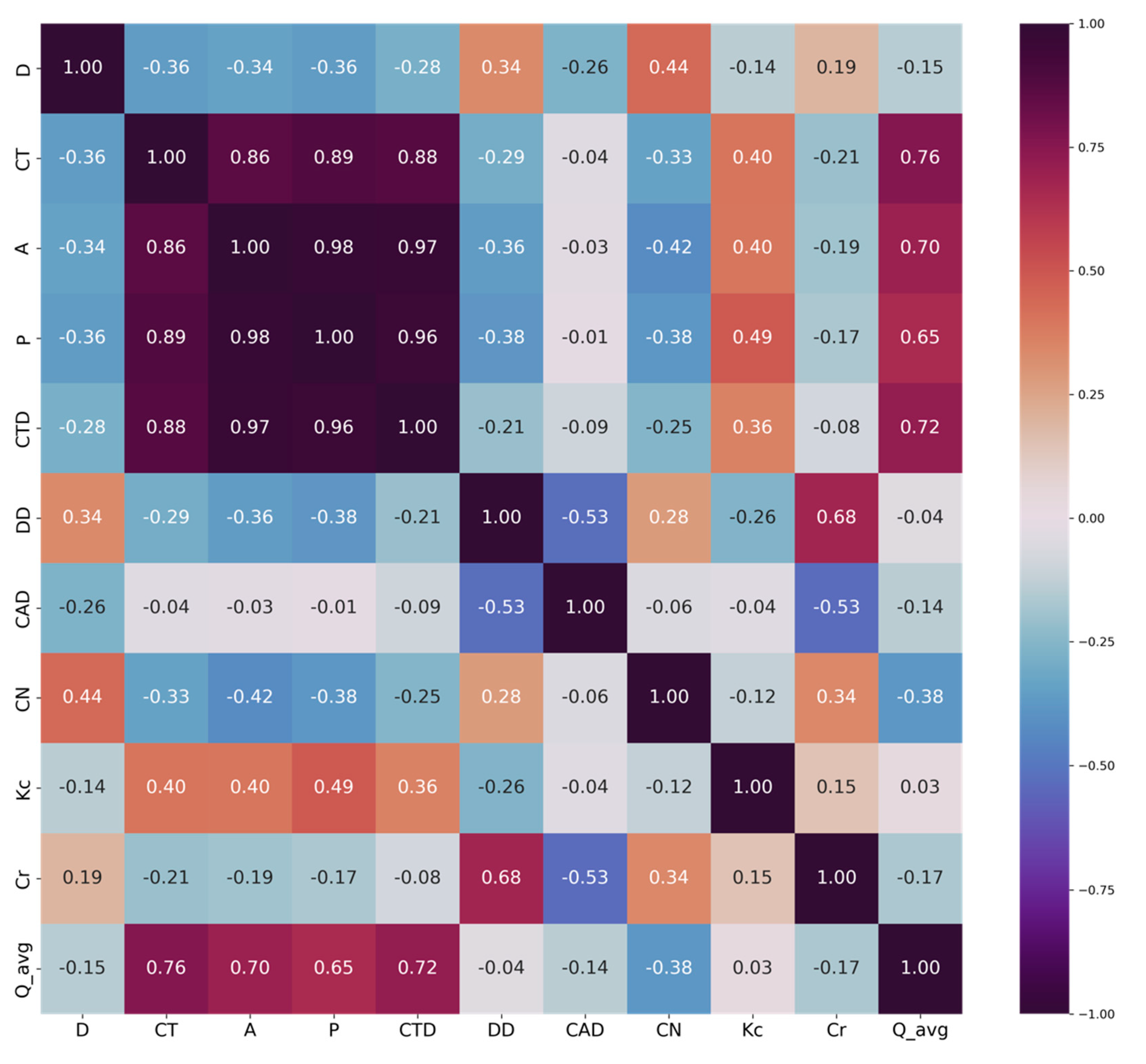
Pearson Correlation Coefficient—Represents the intensity of linear dependency of two variables, it will indicate how similar some of the features are and if they are strongly linear dependent; one of these variables with two features does not need to be included in the model:

$$\mathrm{r}=\frac{{{\displaystyle \sum }}^{ }\left(\mathrm{x}-\overline{\mathrm{x}}\right)\left(\mathrm{y}-\overline{\mathrm{y}}\right)}{\sqrt{{{\displaystyle \sum }}^{ }{\left(\mathrm{x}-\overline{\mathrm{x}}\right)}^2 {{\displaystyle \sum }}^{ }{\left(\mathrm{y}-\overline{\mathrm{y}}\right)}^2}}$$

(11)

• $\mathrm{x}$: Variable 1
• $\mathrm{y}$: Variable 2

2.

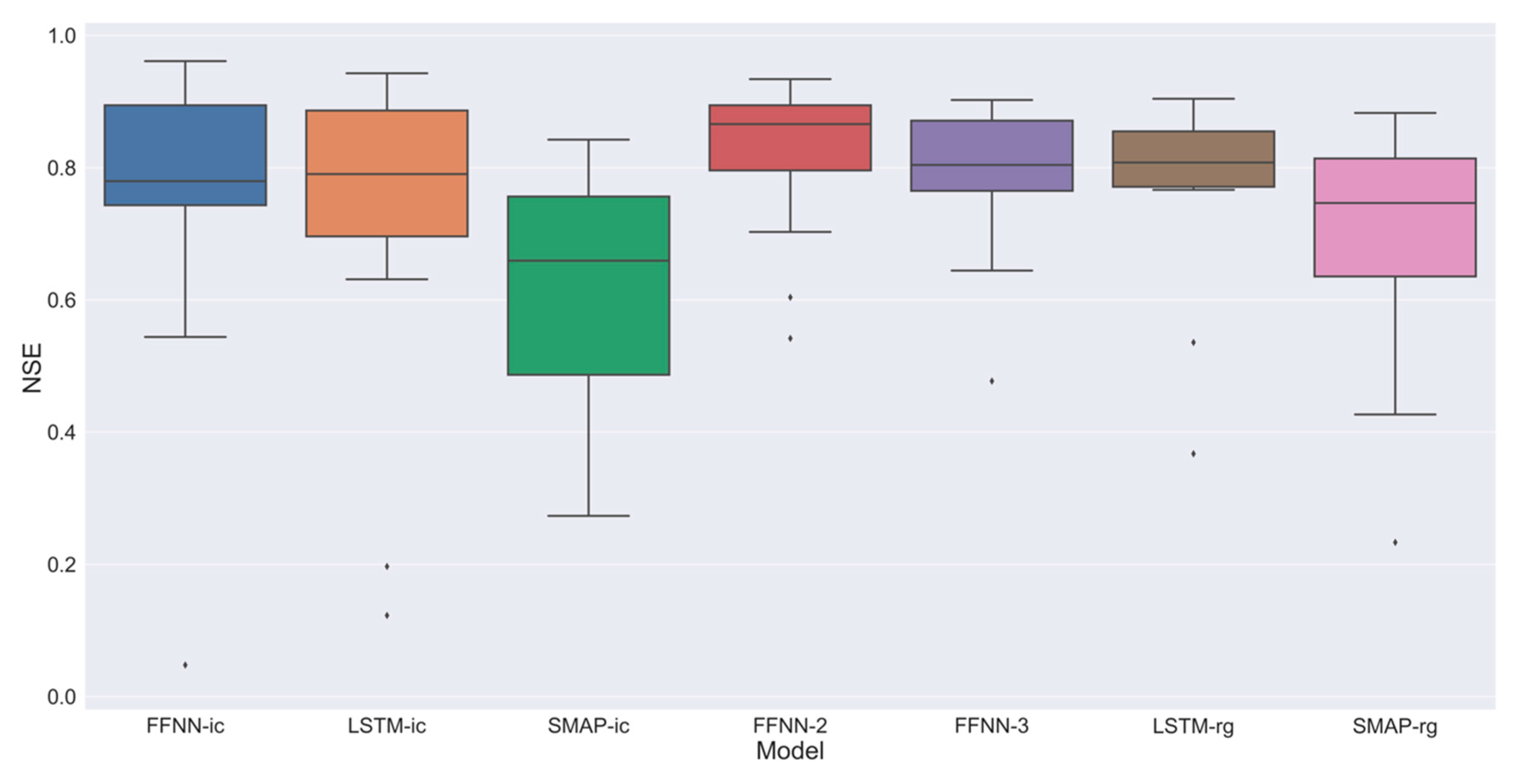
Nash-Sutcliffe Efficiency Coefficient—the index varies from (−∞, 1], values close to 1 indicate that the model fits perfectly with historical series, while values close to 0 would indicate that the model is as representative as the mean. Negative values indicate that the mean is more representative than the model. Its mathematical representation is given by:

$$\mathrm{NSE} =1-\frac{{{\displaystyle \sum }}_{\mathrm{t}=1}^{\mathrm{T}}{\left({\mathrm{Q}}_{\mathrm{m}}^{\mathrm{t}}-{ \mathrm{Q}}_{\mathrm{o}}^{\mathrm{t}}\right)}^2}{{{\displaystyle \sum }}_{\mathrm{t}=1}^{\mathrm{T}}{\left({\mathrm{Q}}_{\mathrm{o}}^{\mathrm{t}}-{\overline{\mathrm{Q}}}_{\mathrm{o}}\right)}^2}$$

(12)

• ${\mathrm{Q}}_{\mathrm{m}}^{\mathrm{t}}$: Modeled discharge at time t
• ${\mathrm{Q}}_{\mathrm{o}}^{\mathrm{t}}$: Observed discharge at time t
• $\overline{{\mathrm{Q}}_{\mathrm{o}}}$: Mean of observed discharges

3.

Root Mean Squared Error—used to indicate the magnitude of the error, and its value represents the average vertical distance between observed and predicted values.

$$\mathrm{RMSE}=\sqrt{ {\displaystyle \sum }_{\mathrm{i}=1}^{\mathrm{n}}\frac{{\left({\overline{\mathrm{y}}}_{\mathrm{i}}-{\mathrm{y}}_{\mathrm{i}}\right)}^2}{\mathrm{n}}}$$

(13)

• ${\mathrm{y}}_{\mathrm{i}}$: Observed value at time i
• $\overline{{\mathrm{y}}_{\mathrm{i}}}$: Predicted value at time i
• n: Number of predictions

4.

Relative Absolute Error—used to indicate a relative measure of the performance of the model with a naïve model that uses only the mean of the observed variable. It is similar to NSE, in a way. If $\mathrm{RAE}\ge 1$, it would be better to use only the mean to describe the target variable:

$$\mathrm{RAE}=\frac{{{\displaystyle \sum }}_{\mathrm{i}=1}^{\mathrm{n}}\left|{\mathrm{y}}_{\mathrm{i}}-\widehat{{\mathrm{y}}_{\mathrm{i}}} \right|}{{{\displaystyle \sum }}_{\mathrm{i}=1}^{\mathrm{n}}\left|{\mathrm{y}}_{\mathrm{i}}-\overline{\mathrm{y}}\right|}$$

(14)

• ${\mathrm{y}}_{\mathrm{i}}$: Observed value at time i
• $\widehat{{\mathrm{y}}_{\mathrm{i}}}$: Predicted value at time i
• $\mathrm{y} ¯$: Average of observed value
• n: Number of pr edictions

3. Results

3.1. Selected Features

Figure 5 indicates the cross-validation scores for each number of features. The optimal number of features is nine and were: Catchment Area (A), Total drainage length (CTD), Longest drainage length (CT), Curve Number (CN), Portion of the basin in the crystalline rock (Cr)—the catchment features, and the monthly average evapotranspiration along with the precipitations of the previous three months as the climate features.

Although the RFECV indicates the optimal number of attributes for the model as nine, it is important to highlight a couple of points: (I) the main gain of information is from one to three attributes and the difference from three to nine is marginal; (II) a non-linear relationship of a feature and the streamflow is not incorporated into the analysis, and (III) a high collinearity among the variables may skew the results, and it may not be necessary to use all of the highly correlated variables in the final model.

Thus, models using sets of three to nine variables were trained with an FFNN and the results obtained with the number with eight features were satisfactory. The final set of attributes were A, CTD, CN, Cr, the monthly average evapotranspiration, and the precipitation of the previous three months.

Figure 6 presents a correlogram of the physiographical characteristics and the average streamflow (Q_avg) of the basins, and indicates that CT, A, P, and CTD are highly correlated. That is in accord with point (III) and can justify removal of CT in the final model.

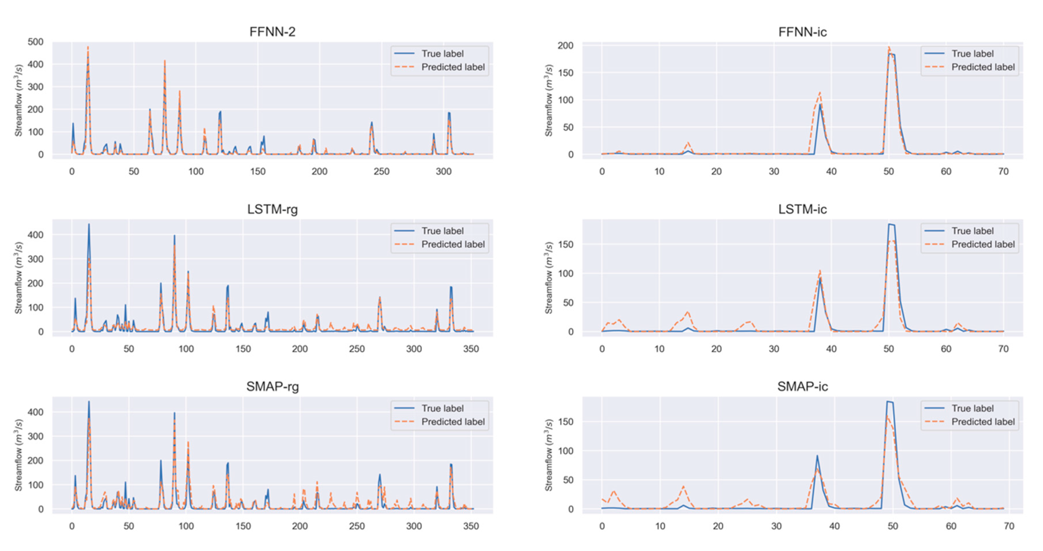
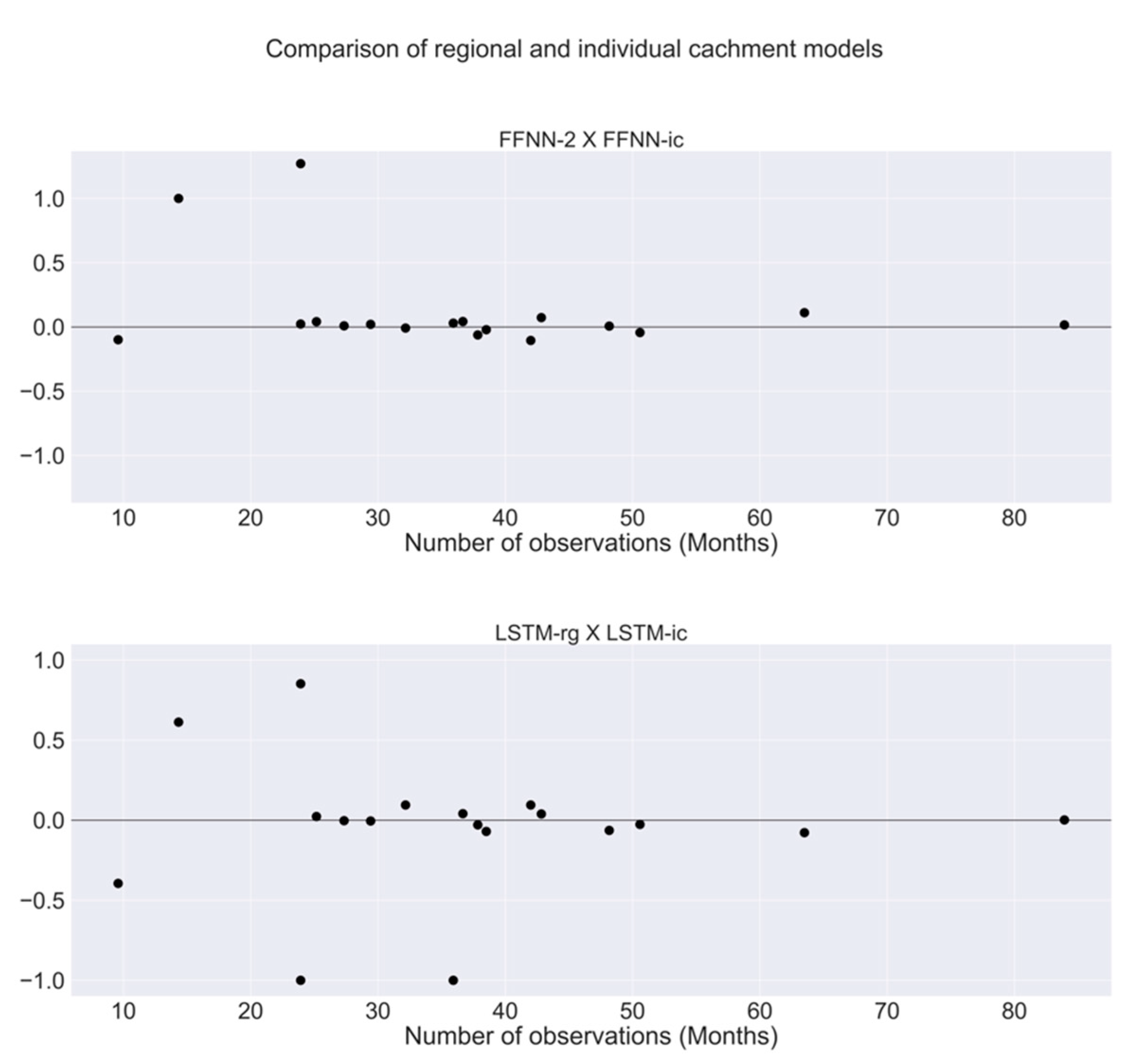
3.2. Results of Models

The results of the different ANN architectures for regional and individual catchment models and SMAP models are presented in

Table 3. Models’ performances per basin.

Basin	n obs	Experiment 1			Experiment 2
		FFNN-ic	LSTM-ic	SMAP-ic	FFNN-2	FFNN-3	LSTM-rg	SMAP-rg
34730000	475	0.192	0.101	−0.304	−3.559	−4.854	−3.216
34740000	92	0.199	0.624	−31.361	0.505	0.440	0.564
34750000	514	0.747	0.751	0.653	0.883	0.881	0.823	0.427
35050000	115	0.680	0.912	0.760	0.542	0.477	0.367	0.233
35125000	328	0.896	0.890	0.814	0.915	0.903	0.885	0.883
35170000	462	0.939	0.923	0.617	0.895	0.863	0.785	0.854
35210000	578	0.910	0.943	0.503	0.925	0.874	0.814	0.806
35223000	130	0.069	0.172	0.230	0.278	0.100	0.182
35240000	421	0.455	0.496	0.538	0.739	0.509	0.615
35260000	504	0.770	0.687	0.666	0.604	0.714	0.855	0.788
35263000	287	0.790	0.817	0.817	0.832	0.805	−0.564	0.817
35668000	319	0.335	0.835	0.019	−0.750	0.151	−1.522
35880000	287	0.048	0.123	0.435	0.893	0.816	0.873	0.748
35950000	386	0.881	0.631	−0.413	0.863	0.760	0.786	0.778
36020000	762	0.544	0.641	0.274	0.703	0.644	0.536	0.602
36125000	440	0.748	0.724	0.481	0.825	0.854	0.795	0.680
36130000	302	0.823	0.858	0.697	0.905	0.901	0.904	0.728
36160000	1007	0.743	0.764	0.686	0.771	0.802	0.767	0.703
36210000	431	0.744	0.728	0.769	0.796	0.755	−0.070	0.613
36250000	454	0.918	0.866	0.281	0.796	0.780	0.810	0.620
36270000	172	−0.871	0.197	0.747	0.875	0.798	0.806	0.745
36290000	607	0.961	0.908	0.843	0.869	0.804	0.854	0.845
36470000	274	0.878	0.790	0.070	0.767	0.432	0.574
36520000	353	0.891	0.875	0.617	0.934	0.898	0.865	0.847

. Due to the negative skewness of the distribution of the NSE, since it varies from (−∞, 1], it was to be used as the median as a measure of central tendency, and the Bootstrap technique was used to obtain the standard error of the medians for a 95% confidence interval. These results are shown in

Table 4. Median of models’ performances.

Metrics	FFNN-ic	LSTM-ic	SMAP-ic	FFNN-2	FFNN-3	LSTM-rg	SMAP-rg
NSE	0.780 ± 0.091	0.790 ± 0.105	0.659 ± 0.103	0.866 ± 0.045	0.804 ± 0.045	0.808 ± 0.055	0.747 ± 0.07
RMSE (m3/s)	10.197 ± 3.548	9.706 ± 4.692	11.282 ± 3.990	10.765 ± 6.243	12.541 ± 6.617	11.730 ± 6.532	14.670 ± 7.213
RAE (%)	0.325 ± 0.088	0.350 ± 0.057	0.466 ± 0.071	0.306 ± 0.050	0.344 ± 0.040	0.374 ± 0.091	0.414 ± 0.046

along with the Bootstrapped results of RMSE and RAE. The RMSE and RAE values for both SMAP models are empty since these metrics were not used in Ref. [33]. For this, 1000 bootstrapped datasets were used. Moreover, aiming to obtain a fairer comparison, only the results of basins used on the regionalization step in Barros et al. [33] were compared.

Regarding the individual catchment models (experiment 1), both ANN models outperformed the conceptual model SMAP in all three metrics. The LSTM outperform the FFNN in two of the three metrics, presenting a lower error in magnitude, but higher in relative difference. As shown in Figure 7, increasing the number of observations tends to converge performance. When both models obtained a negative value of NSE, it was considered a “tie”, regardless of the magnitude of the value, since by design, a negative value of NSE represents that the model has a worse predicting performance than the simple use of the series average. When a model had an $\mathrm{NSE} >0$ and the other had an $\mathrm{NSE} \le 0$, the score was 1 or −1, depending on if the model is in numerator or denominator, respectively. In smaller series, the NSE tends to be zero and small variations may give the impression that one model is strongly superior to the other, even if the difference is marginal; this particularity can be observed in Figure 7.

For the regional models in experiment 2, Figure 8 indicates that the LSTM performed equally to the FFNN, but with a smaller variance, when the models used the same inputs. Although, when streamflow’s lag is used as input for the FFNN, the FFNN model becomes the one with the better performance in this study. Equally as experiment 1, all the neural network models performed better than the benchmark model, and they also presented a smaller variance. This also supports the idea that neural networks may be better in streamflow regionalization than conceptual models, at least for the case study.

The model FFNN-2, on average, performed better than all others. As Table 4 shows, the LSTM can perform better or not than the Feedforward models depending on the composition of the FFNN. This result may be answered by the fact that as the model became deeper, with more neurons and more complex architecture, it became harder to train its parameters and define its hyperparameters for data available.

Once both models are equally simple, the recurrent model scored negative fewer times and presented the smallest magnitude error, evidencing that using recurrence may increase the model’s performance, but these gains are not so significant. Figure 7 also shows that the increasing of observations converged the individual catchment model’s performance.

Figure 9 compares the regional models FFNN-2 and FFNN-3 with LSTM-rg and SMAP while Figure 10 compares model FFNN-2 with LSTM-rg for the different basin characteristics. It is possible to see, from Figure 9, that both Feedforward models outperform the Recurrent, and Figure 10 shows that the basin composition does not explain the difference of a model’s performance; even though it is expected that the LSTM learn the short- and long-time dependencies, this does not convert into informational gains. A possible explanation is that the hydrological memory in the region is considerably short, due to its location in semiarid weather and shallow soil composition.

In Figure 11, it is possible to see that FFNN-2 tends to outperform FFNN-ic considerably better in the first 25 years of data, but this difference tends to decrease with the increase in data availability for the individual catchment models. The same tendency can be observed when comparing the LSTMs’ regional and individual catchment models. This corroborates to the hypothesis that for basins with low data availability, a data-driven streamflow regionalization approach may perform better than an individual catchment hydrological model approach.

Figure 12 illustrates the difference of predicted values versus the measured values for streamflow discharge of basin 36520000 of regional and individual catchment models in the validation set; since the regional models use the entire series for validation and the individual catchment only the last 20%, the time series length were different. The series for the FFNN-2 model was also smaller than the rest of the regional models because it uses the discharges as input, so any measured value error that was discarded would discount three instances in the dataset. In the graph, is possible to observe that the Feedforward models correctly predict peak discharges in location and intensity, whereas the LSTM and SMAP models, sometimes, predict a discharge peak when it does not occur.

4. Discussion

The LSTM cells demonstrated their capacity to explain the hydrological process of streamflow in semiarid regions, performing better than the Feedforward model in the individual catchment and the conceptual model in both experiments. Regarding the Feedforward models in regionalization, when using the same input set, both models have practically the same performance (LSTM-rg: NSE = 0.808, RMSE = 11.730 m³/s, RAE = 0.374; FFNN-3: NSE = 0.804, RMSE = 12.541 m³/s, RAE = 0.344). However, the use of streamflow lags proved to be the single major increment of models’ performances (FFNN-2: NSE = 0.866, RMSE = 10.765 m³/s, RAE = 0.306). It is important to point out that FFNN-2 and FFNN-3 use less parameters, 3151 and 3051, respectively, than the LSTM-rg, 4491, so it performs as good or as better with least computational cost.

The results of this study are also in accord with what we find in the literature. As mentioned in the introduction, Ref. [28] found that LSTM cells performed better for snow-driven than for arid catchments. In the context of Evapotranspiration, Ref. [53] showed that LSTM-based models outperformed NARX-based models in the humid, subtropical climate of southern Florida but underperformed the latter for the semiarid climate of Central Nevada.

The aforementioned may be due to the fact the rainfall-runoff hydrological memory in regions such as the State of the Ceará is short due to its semiarid weather, its shallow soil, and the diminished baseflow, decreasing the importance of the long-term memory if compared with short-term memory. Furthermore, the increasing number of parameters required by the use of LSTM cells increases the difficulty to train the ANN for the available observed data which is not justified without a gain of information or performance. Although, this does not mean that the use of LSTM cells should not be used in semiarid regions as Ref. [54] used a hybrid Bi-LSTM for the forecast of short-term daily reference under limited meteorological variables, and other studies found that LSTM performed better than three benchmark models for drought modeling by standard precipitation index (SPI) in a daily series of four Iranian stations [55].

For the individual catchment models, even with the embedded information in the structure of the conceptual models regarding the hydrological process, the ANNs performed better for this region with data scarcity.

Comparing the results, we see that the decrease of variables improved the performance of the network. In this case, Contribution area of the fluviometric station (A), Total drainage length (CTD), Average Curve Number (CN), and Portion of the basin in the crystalline bedrock (Cr) can represent basins located on semiarid regions with high fidelity, since A and CTD influences the dimension of the water volume presented on each catchment while CN and Cr represent the soil storage capacity and infiltration-runoff relationships.

It is important to highlight that the two basins with the smallest portion of the basin in the crystalline rock (34730000, 34740000) and the basin with the smallest area (35668000) performed poorly compared to the others, which may indicate that hydrological processes of these basins are different from the others.

Although ANNs involve more complex concepts, the use of modern frameworks such as Tensorflow make ANN models significantly easier to train and to be implemented. Beyond that, ANNs are more scalable, allowing the use of a pre-trained model to regionalize an entire region, even for a site extremely poor in data.

Furthermore, as SMAP and other conceptual models’ regionalization procedure evaluates the streamflow with a two-step method (i.e., it first estimates its parameters for the observed basins and later regionalizes the value of the parameters for the whole region), the procedure is submitted to two uncertainty causes: the intrinsic uncertainty of the conceptual model and the uncertainty generated by the regionalization of its parameters, while the ANN models are only subjected to the first uncertainty.

From the comparison between the ANN regional and individual catchment models, it is notable that for catchments with less than 25 years of streamflow records, the regional model outperforms the individual catchment model. This fact implies that for certain regions, with some well-documented catchments, the use of an ANN regional model can be more economically efficient for WRPM and perform better than setting up a new fluviometric station on an ungauged basin for a substantial amount of time records. For regions such as the State of Ceará, located in the semiarid region with poor fluviometric stations data, but with a wide coverage area of pluviometric stations, the use of ANN models may assist governments and civil institutions in the WRPM with low implementation costs.

5. Conclusions

An accurate prediction of streamflow in ungauged basins is essential for water resources planning and management. The advance of powerful computers allowed us to explore the potential of Deep Learning in Hydrology. In this paper, we presented an application of LSTM as a streamflow regionalization method for a case study with strong challenges: reduced data availability and harsh hydrological conditions, such as intermittent rivers, high precipitation variability, and catchments with shallow soil characteristics. Its performance was analyzed against a traditional Feedforward ANN and conceptual models to evaluate if it is a suitable and robust streamflow model and a regionalization method for a semiarid region.

In general, all ANNs used for regionalization outperformed the benchmark model, including the LSTM, although its use was not justified since its performance was as good as the FFNN-3, a model that used the same inputs, and inferior to FFNN-2, that used the previous two months of streamflow lags. In the comparison with FFNN-2, the difference in the basin’s characteristics did not influence the model’s performance, possibly because, in general, the basins used in this study are homogeneous. Both FFNN-ic and LSTM-ic were able to outperform the benchmark model, and the LSTM-ic performed better than FFNN-ic.

As for the applicability of LSTM for streamflow regionalization in a semiarid region, although performing good, this study showed that a simpler ANN may be a choice as good as or, with small changes, can outperform the LSTM.

The data limitation seems to be a major drawback for the use of LSTM architecture in our study, so we encourage other researchers to implement a streamflow regional LSTM model for other semiarid regions with larger datasets or to use hybrid methods with LSTM and other models for regionalization of ungauged basins in a different timescale. The use of new ANN architectures such as Transformers are also encouraged to be implemented as a model for streamflow regionalization.

The results obtained by this study can be extended to most of the Brazilian Northeastern semiarid region as its overall characteristics are very similar to the region used in this case study.

References

1. Freire-González, J.; Decker, C.; Hall, J.W. The Economic Impacts of Droughts: A Framework for Analysis. Ecol. Econ. 2017, 132, 196–204. [Google Scholar] [CrossRef]
2. Mosley, L.M. Drought Impacts on the Water Quality of Freshwater Systems; Review and Integration. Earth-Science Rev. 2015, 140, 203–214. [Google Scholar] [CrossRef]
3. Clark, J.S.; Iverson, L.; Woodall, C.W.; Allen, C.D.; Bell, D.M.; Bragg, D.C.; D’Amato, A.W.; Davis, F.W.; Hersh, M.H.; Ibanez, I.; et al. The Impacts of Increasing Drought on Forest Dynamics, Structure, and Biodiversity in the United States. Glob. Chang. Biol. 2016, 22, 2329–2352. [Google Scholar] [CrossRef] [Green Version]
4. Kirchner, J.W. Getting the Right Answers for the Right Reasons: Linking Measurements, Analyses, and Models to Advance the Science of Hydrology. Water Resour. Res. 2006, 42, 1–5. [Google Scholar] [CrossRef]
5. Wood, E.F.; Roundy, J.K.; Troy, T.J.; Van Beek, L.P.H.; Bierkens, M.F.; Blyth, E.; De Roo, A.; Döll, P.; Ek, M.; Famiglietti, J.; et al. Hyperresolution global land surface modeling: Meeting a grand challenge for monitoring Earth’s terrestrial water. Water Resour. Res. 2011, 47, W05301. [Google Scholar] [CrossRef]
6. Clark, M.P.; Bierkens, M.F.P.; Samaniego, L.; Woods, R.A.; Uijenhoet, R.; Bennet, K.E.; Pauwels, V.R.N.; Cai, X.; Wood, A.W.; Peters-Lidard, C.D. The Evolution of Process-Based Hydrologic Models: Historical Challenges and the Collective Quest for Physical Realism. Hydrol. Earth Syst. Sci. 2017, 21, 3427–3440. [Google Scholar] [CrossRef] [Green Version]
7. Fowler, K.J.A.; Peel, M.C.; Western, A.W.; Zhang, L.; Peterson, T.J. Simulating Runoff under Changing Climatic Conditions: Revisiting an Apparent Deficiency of Conceptual Rainfall-Runoff Models. Water Resour. Res. 2016, 52, 1820–1846. [Google Scholar] [CrossRef] [Green Version]
8. Herrnegger, M.; Senoner, T.; Nachtnebel, H.P. Adjustment of Spatio-Temporal Precipitation Patterns in a High Alpine Environment. J. Hydrol. 2018, 556, 913–921. [Google Scholar] [CrossRef]
9. Govindaraju, R.S.; Rao, A.R. Artificial Neural Networks in Hydrology; Springer Science & Business Media: Berlin/Heidelberg, Germany, 2013; Volume 36. [Google Scholar]
10. Her, Y.; Yoo, S.H.; Cho, J.; Hwang, S.; Jeong, J.; Seong, C. Uncertainty in Hydrological Analysis of Climate Change: Multi-Parameter vs. Multi-GCM Ensemble Predictions. Sci. Rep. 2019, 9, 4974. [Google Scholar] [CrossRef] [Green Version]
11. Sivapalan, M.; Takeuchi, K.; Franks, S.W.; Gupta, V.K.; Karambiri, H.; Lakshmi, V.; Liang, X.; McDonnell, J.J.; Mendiondo, E.M.; O’Connell, P.E.; et al. IAHS Decade on Predictions in Ungauged Basins (PUB), 2003-2012: Shaping an Exciting Future for the Hydrological Sciences. Hydrol. Sci. J. 2003, 48, 857–880. [Google Scholar] [CrossRef] [Green Version]
12. Croke, B.F.W.; Merritt, W.S.; Jakeman, A.J. A Dynamic Model for Predicting Hydrologic Response to Land Cover Changes in Gauged and Ungauged Catchments. J. Hydrol. 2004, 291, 115–131. [Google Scholar] [CrossRef]
13. Götzinger, J.; Bárdossy, A. Comparison of Four Regionalisation Methods for a Distributed Hydrological Model. J. Hydrol. 2007, 333, 374–384. [Google Scholar] [CrossRef]
14. Oudin, L.; Andréassian, V.; Perrin, C.; Michel, C.; Le Moine, N. Spatial Proximity, Physical Similarity, Regression and Ungaged Catchments: A Comparison of Regionalization Approaches Based on 913 French Catchments. Water Resour. Res. 2008, 44, 1–15. [Google Scholar] [CrossRef]
15. Merz, R.; Blöschl, G. Regionalisation of Catchment Model Parameters. J. Hydrol. 2004, 287, 95–123. [Google Scholar] [CrossRef] [Green Version]
16. Post, D.A. Regionalizing Rainfall-Runoff Model Parameters to Predict the Daily Streamflow of Ungauged Catchments in the Dry Tropics. Hydrol. Res. 2009, 40, 433–444. [Google Scholar] [CrossRef]
17. Li, H.; Zhang, Y.; Chiew, F.H.S.; Xu, S. Predicting Runoff in Ungauged Catchments by Using Xinanjiang Model with MODIS Leaf Area Index. J. Hydrol. 2009, 370, 155–162. [Google Scholar] [CrossRef]
18. Samuel, J.; Coulibaly, P.; Metcalfe, R.A. Estimation of Continuous Streamflow in Ontario Ungauged Basins: Comparison of Regionalization Methods. J. Hydrol. Eng. 2011, 16, 447–459. [Google Scholar] [CrossRef]
19. Zhang, Y.; Chiew, F.H.S. Relative Merits of Different Methods for Runoff Predictions in Ungauged Catchments. Water Resour. Res. 2009, 45, W07412. [Google Scholar] [CrossRef]
20. McCabe, M.F.; Franks, S.W.; Kalma, J.D. Calibration of a Land Surface Model Using Multiple Data Sets. J. Hydrol. 2005, 302, 209–222. [Google Scholar] [CrossRef]
21. Sefton, C.E.M.; Howarth, S.M. Relationships between Dynamic Response Characteristics and Physical Descriptors of Catchments in England and Wales. J. Hydrol. 1998, 211, 1–16. [Google Scholar] [CrossRef]
22. Lee, H.; McIntyre, N.R.; Wheater, H.S.; Young, A.R. Predicting Runoff in Ungauged UK Catchments. Proc. Inst. Civ. Eng. Water Manag. 2006, 159, 129–138. [Google Scholar] [CrossRef] [Green Version]
23. Besaw, L.E.; Rizzo, D.M.; Bierman, P.R.; Hackett, W.R. Advances in Ungauged Streamflow Prediction Using Artificial Neural Networks. J. Hydrol. 2010, 386, 27–37. [Google Scholar] [CrossRef]
24. Heuvelmans, G.; Muys, B.; Feyen, J. Regionalisation of the Parameters of a Hydrological Model: Comparison of Linear Regression Models with Artificial Neural Nets. J. Hydrol. 2006, 319, 245–265. [Google Scholar] [CrossRef]
25. Fathian, F.; Mehdizadeh, S.; Kozekalani Sales, A.; Safari, M.J.S. Hybrid Models to Improve the Monthly River Flow Prediction: Integrating Artificial Intelligence and Non-Linear Time Series Models. J. Hydrol. 2019, 575, 1200–1213. [Google Scholar] [CrossRef]
26. Safari, M.J.S.; Rahimzadeh Arashloo, S.; Danandeh Mehr, A. Rainfall-Runoff Modeling through Regression in the Reproducing Kernel Hilbert Space Algorithm. J. Hydrol. 2020, 587, 125014. [Google Scholar] [CrossRef]
27. Shen, C. A Transdisciplinary Review of Deep Learning Research and Its Relevance for Water Resources Scientists. Water Resour. Res. 2018, 54, 8558–8593. [Google Scholar] [CrossRef]
28. Kratzert, F.; Klotz, D.; Brenner, C.; Schulz, K.; Herrnegger, M. Rainfall-Runoff Modelling Using Long Short-Term Memory (LSTM) Networks. Hydrol. Earth Syst. Sci. 2018, 22, 6005–6022. [Google Scholar] [CrossRef] [Green Version]
29. Hu, C.; Wu, Q.; Li, H.; Jian, S.; Li, N.; Lou, Z. Deep Learning with a Long Short-Term Memory Networks Approach for Rainfall-Runoff Simulation. Water 2018, 10, 1543. [Google Scholar] [CrossRef] [Green Version]
30. Xiang, Z.; Yan, J.; Demir, I. A Rainfall-Runoff Model with LSTM-Based Sequence-to-Sequence Learning. Water Resour. Res. 2020, 56, e2019WR025326. [Google Scholar] [CrossRef]
31. Fan, H.; Jiang, M.; Xu, L.; Zhu, H.; Cheng, J.; Jiang, J. Comparison of Long Short Term Memory Networks and the Hydrological Model in Runoff Simulation. Water 2020, 12, 175. [Google Scholar] [CrossRef] [Green Version]
32. Addor, N.; Newman, A.J.; Mizukami, N.; Clark, M.P. The CAMELS data set: Catchment attributes and meteorology for large-sample studies. Hydrol. Earth Syst. Sci. 2017, 21, 5293–5313. [Google Scholar] [CrossRef] [Green Version]
33. Barros, F.; Martins, E.; Souza Filho, F.A. Regionalização de parâmetros do modelo chuva-vazão SMAP das bacias hidrográficas do Ceará. In Gerenciamento de Recursos Hídricos no Semiárido; Expressão Gráfica e Editora: Fortaleza, Brazil, 2013. [Google Scholar]
34. Abadi, M.; Agarwal, A.; Barham, P.; Brevdo, E.; Chen, Z.; Citro, C.; Zheng, X. Tensorflow: Large-scale machine learning on heterogeneous distributed systems. arXiv Prepr. 2016, arXiv:1603.04467. [Google Scholar]
35. Lopes, J.E.G.; Braga, B.P.F., Jr.; Conejo, J.G.L. SMAP—A Simplified Hydrologic Model. Appl. Modeling Catchment Hydrol. 1982, 167–176. Available online: https://agris.fao.org/agris-search/search.do?request_locale=ar&recordID=US201302608054&query=&sourceQuery=&sortField=&sortOrder=&agrovocString=&advQuery=&centerString=&enableField= (accessed on 16 March 2022).
36. Companhia de Gestão dos Recursos Hídricos (COGERH). Estudos de Regionalização de Parâmetros de Modelo Hidrológico Chuva-Vazão, Para as Bacias Totais e Incrementais dos Reservatórios Monitorados Pela COGERH; COGERH: Fortaleza, Brazil, 2013. [Google Scholar]
37. Alexandre, A.M.B.; Martins, E.S.; Clarke, R.T.; Reis, D.S., Jr. Regionalização de parâmetros de modelos hidrológicos. In Anais do XVI Simpósio Brasileiro de Recursos Hídricos; ABRH, João Pessoa–PB, 2005; Available online: http://www.funceme.br/produtos/manual/acudes_e_rios/Regionalizacao/textos/RegSMAP_PaperABRH.pdf (accessed on 16 March 2022).
38. Nascimento, L.S.V.; Reis, D.S., Jr.; Martins, E.S.P. Avaliação do algoritmo evolutivo Mopso na calibração multiobjetivo do modelo SMAP no estado do Ceará. Diretoria da ABRH 2009, 14, 85–97. [Google Scholar] [CrossRef]
39. Block, P.J.; Souza Filho, F.A.; Sun, L.; Kwon, H.H. A Streamflow Forecasting Framework Using Multiple Climate and Hydrological Models. J. Am. Water Resour. Assoc. 2009, 45, 828–843. [Google Scholar] [CrossRef]
40. Barros, M.T.L.; Lopes, J.E.G.; Zambon, R.C.; Francato, A.L.; Barbosa, P.S.F.; Zanfelice, F.R. Climate Flow Forecast Model for the Brazilian Hydropower System. In Proceedings of the World Environmental and Water Resources Congress 2009: Great Rivers, Kansas City, MO, USA, 17–21 May 2009; Volume 342, pp. 4727–4735. [Google Scholar] [CrossRef]
41. Da Silva, F.D.N.R.; Alves, J.L.D.; Cataldi, M. Climate Downscaling over South America for 1971–2000: Application in SMAP Rainfall-Runoff Model for Grande River Basin. Clim. Dyn. 2019, 52, 681–696. [Google Scholar] [CrossRef]
42. McCulloch, W.S.; Pitts, W. A logical calculus of the ideas immanent in nervous activity. Bull. Math. Biophys. 1943, 5, 115–133. [Google Scholar] [CrossRef]
43. Haykin, S. Neural Networks: A Comprehensive Foundation; Maemillan: New York, NY, USA, 1994; p. 696. [Google Scholar]
44. Hochreiter, S.; Schmidhuber, J. Long Short-Term Memory. Neural Comput. 1997, 9, 1735–1780. [Google Scholar] [CrossRef]
45. Elman, J.L. Finding Structure in Time. Cogn. Sci. 1990, 14, 179–211. [Google Scholar] [CrossRef]
46. Hochreiter, S. The Vanishing Gradient Problem during Learning Recurrent Neural Nets and Problem Solutions. Int. J. Uncertain. Fuzziness Knowl.-Based Syst. 1998, 6, 107–116. [Google Scholar] [CrossRef] [Green Version]
47. Guyon, I.; Weston, J.; Barnhill, S.; Vapnik, V. Gene selection for cancer classification using support vector machines. Mach. Learn. 2002, 46, 389–422. [Google Scholar] [CrossRef]
48. Parajka, J.; Merz, R.; Blöschl, G. A Comparison of Regionalisation Methods for Catchment Model Parameters. Hydrol. Earth Syst. Sci. 2005, 9, 157–171. [Google Scholar] [CrossRef] [Green Version]
49. Laaha, G.; Blöschl, G. A Comparison of Low Flow Regionalisation Methods-Catchment Grouping. J. Hydrol. 2006, 323, 193–214. [Google Scholar] [CrossRef]
50. Leclerc, M.; Ouarda, T.B.M.J. Non-Stationary Regional Flood Frequency Analysis at Ungauged Sites. J. Hydrol. 2007, 343, 254–265. [Google Scholar] [CrossRef]
51. Hinton, G.; Srivastava, N.; Swersky, K. Neural networks for machine learning lecture 6a overview of mini-batch gradient descent. Cited 2012, 14, 2. [Google Scholar]
52. Srivastava, N.; Hinton, G.; Krizhevsky, A.; Sutskever, I.; Salakhutdinov, R. Dropout: A Simple Way to Prevent Neural Networks from Overfitting. J. Mach. Learn. Res. 2014, 15, 1929–1958. [Google Scholar]
53. Granata, F.; Di Nunno, F. Forecasting Evapotranspiration in Different Climates Using Ensembles of Recurrent Neural Networks. Agric. Water Manag. 2021, 255, 107040. [Google Scholar] [CrossRef]
54. Yin, J.; Deng, Z.; Ines, A.V.M.; Wu, J.; Rasu, E. Forecast of Short-Term Daily Reference Evapotranspiration under Limited Meteorological Variables Using a Hybrid Bi-Directional Long Short-Term Memory Model (Bi-LSTM). Agric. Water Manag. 2020, 242, 106386. [Google Scholar] [CrossRef]
55. Docheshmeh Gorgij, A.; Alizamir, M.; Kisi, O.; Elshafie, A. Drought Modelling by Standard Precipitation Index (SPI) in a Semi-Arid Climate Using Deep Learning Method: Long Short-Term Memory. Neural Comput. Appl. 2022, 34, 2425–2442. [Google Scholar] [CrossRef]
Figure 1. Studied catchments.
Water 14 01318 g001
Figure 2. Graphical representation of an LSTM Cell.
Water 14 01318 g002
Figure 3. Data processing flowchart for FFNN-3 regionalization model. “None” represents the batch size, which is only decided in the training phase.
Water 14 01318 g003
Figure 4. Data processing flowchart for the LSTM model. “None” represents the batch size, which is only decided in the training phase.
Water 14 01318 g004
Figure 5. Recursive Feature Elimination performance vs. number of features.
Water 14 01318 g005
Figure 6. Features Pearson correlation coefficient heatmap.
Water 14 01318 g006
Figure 7. The y-axis represents the logarithm of the ratio of the NSE index of the LSTM-ic over the NSE from the FFNN-ic model against the number of data observations in years in each basin (x-axis).
Water 14 01318 g007
Figure 8. Boxplot comparing models’ performance.
Water 14 01318 g008
Figure 9. The y-axis represents the logarithm of the ratio of the NSE index of the FFNN-2 and FFNN-3 over the NSE index from the LSTM-rg and SMAP for all basins in the subset “iii” (x-axis).
Water 14 01318 g009
Figure 10. The y-axis represents the logarithm of the ratio of the NSE index of the FFNN-2 over the NSE index from the LSTM-rg model for each basin’s characteristics used in this study (x-axis).
Water 14 01318 g010
Figure 11. The y-axis represents the logarithm of ratio of the NSE index of the FFNN-2 and LSTM-ic over the NSE index from the FFNN-ic and LSTM-ic models, respectively, against the number of data observations in the basin (x-axis).
Water 14 01318 g011
Figure 12. Time series of expected and measured values for basin 36520000.
Water 14 01318 g012