An Improved Transfer Learning Model for Cyanobacterial Bloom Concentration Prediction

Abstract

The outbreak of cyanobacterial blooms is a serious water environmental problem, and the harm it brings to aquatic ecosystems and water supply systems cannot be underestimated. It is very important to establish an accurate prediction model of cyanobacterial bloom concentration, which is a challenging issue. Machine learning techniques can improve the prediction accuracy, but a large amount of historical monitoring data is needed to train these models. For some waters with an inconvenient geographical location or frequent sensor failures, there are not enough historical data to train the model. To deal with this problem, a fused model based on a transfer learning method is proposed in this paper. In this study, the data of water environment with a large amount of historical monitoring data are taken as the source domain in order to learn the knowledge of cyanobacterial bloom growth characteristics and train the prediction model. The data of the water environment with a small amount of historical monitoring data are taken as the target domain in order to load the model trained in the source domain. Then, the training set of the target domain is used to participate in the inter-layer fine-tuning training of the model to obtain the transfer learning model. At last, the transfer learning model is fused with a convolutional neural network to obtain the prediction model. Various experiments are conducted for a 2 h prediction on the test set of the target domain. The results show that the proposed model can significantly improve the prediction accuracy of cyanobacterial blooms for the water environment with a low data volume.

1. Introduction

Excessive nitrogen and phosphorus elements in the water environment will cause water eutrophication [1]. In this eutrophic water environment, cyanobacteria will overproduce, which is called an outbreak of cyanobacterial blooms. The harm of this is huge: the visible harm is that the water body becomes green and smelly, affecting the water appearance and water quality; the invisible harm is that cyanobacterial blooms produce harmful toxins [2,3], poisoning fish and shrimp and other aquatic plants in the aquatic environment, as well as humans and animals [4,5], bringing huge losses to the farming industry and normal production life.

In the past 30 years, harmful algal blooms (HABs) have occurred frequently in China’s coastal waters, resulting in economic losses of more than CNY 5.9 billion due to massive fish and shellfish kills and negative impacts on tourism [6]. Aguilera et al. [7] searched the published literature on the occurrence of cyanobacterial blooms and cyanobacterial toxins and found a total of 241 bloom events between 1994 and 2014 in Argentina. Gorham et al. [8] found a significant positive correlation between drinking water sources impacted by cyanobacterial blooms and hepatocellular carcinoma incidence rates. If the cyanobacterial bloom concentration can be accurately predicted in advance, the prevention and control measures can be deployed in advance, and the supply of alternate drinking water sources can be carried out to minimize the harm that cyanobacterial blooms may produce. Therefore, the prediction of cyanobacterial bloom concentration has been a research topic of interest to scholars.

The challenge of accurate prediction for cyanobacterial bloom concentration is two-fold. On the one hand, there are many factors affecting the growth of cyanobacteria, such as the water temperature, pH, water conductivity, turbidity, etc. [9]. The key to solve this problem is to determine the magnitude of the influence of external factors on the growth of cyanobacteria, which can be obtained by the correlation among the sequence of external factors. On the other hand, the growth changes in cyanobacteria are irregular and easily affected by external factors [10]. Traditional prediction methods include nutrient models based on cyanobacterial growth mechanisms [11,12] and ecodynamic models [13,14]. Nutrient salt models consider the interaction between algal biomass changes and nutrients and judge the water quality by the obtained cyanobacterial biomass changes. These traditional models are not applicable to waters with a large spatial–geographic extent. Ecodynamic models, such as WASP (Water Quality Analysis Simulation Program), EFDC (Environmental Fluid Dynamics Code), and CE-QUAL-W2 (two dimensional hydrodynamic and water quality model) [15], consider the effects of physical, chemical, and biological processes on the water ecosystem and simulate the dynamic changes in algae. These models can reflect the growth characteristics and patterns of algae, which are of great significance for understanding and preventing cyanobacterial bloom outbreaks. However, these models have a large number of parameters to be estimated, require actual data of the water ecosystem for parameter optimization rate determination, and are more dependent on experience.

Recently, artificial intelligence models have been applied to the field of cyanobacterial bloom concentration prediction. Artificial neural networks (ANN) have greater advantages for analyzing complex data [16,17,18] and can provide effective solutions to nonlinear problems. For example, Recknage et al. [19] developed an artificial neural network prediction model using historical data on algal biomass and external driving variables observed in four different freshwater lake systems. Hill et al. [20] developed a detection and prediction system for harmful algal blooms based on a convolutional neural network (CNN) to monitor Mexican waters using remote sensing short-term data. Cho et al. [21] applied the long short-term memory (LSTM) networks to predict the concentration of chlorophyll-a (a recognized characterization of algal activity) using the daily water quality data as input, which showed a better performance in 4-day and 1-day prediction tasks. These models all demonstrate the excellent ability of deep learning methods for algal bloom prediction. However, all of these models require a large amount of historical data to train in order to obtain accurate models. Regardless, there exist some water areas where the amount of monitoring data obtained is relatively small due to an inconvenient location, late start of monitoring, or frequent sensor failures. Thus, it is difficult to train accurate prediction models for these water areas with a low data volume.

Transfer learning is the approach that can address the problem introduced above. The concept of transfer learning is to apply knowledge or patterns learned in one task to different but related tasks so that these tasks can be solved more effectively and efficiently. For example, Wu et al. [22] proposed a method combining industry chain information transfer learning with a deep learning model to predict stock quotes, which improved the prediction accuracy of a target stock market index. Grubinger et al. [23] proposed an online transfer learning framework for predicting residential temperatures that significantly improved the prediction accuracy using data from just a few weeks before new construction. Hu et al. [24] applied transfer learning techniques to predict short-term wind speeds on newly built farms using data training from data-rich farms. These above literatures prove the effectiveness of the transfer learning, especially in the case of a small amount of data.

Based on the idea of transfer learning, Tian et al. [25] presented a transfer-learning-based neural network model for chlorophyll-a dynamics prediction in an estuary reservoir in eastern China for a long-term application, under a small-time interval condition. Different from the literature [25], we propose a prediction method based on transfer learning to solve the problem of a small amount of data in some water areas. When the amount of data in the target domain is small, the model cannot be well trained by only using the data in the target domain. However, the knowledge of the cyanobacteria bloom growth in different water areas is similar. Thus, the motivation of this study is to fine-tune by freezing some parameters of the model to realize the prediction of cyanobacterial bloom concentration across different water regions. In addition, to reduce the effects of diversities of different water areas, the prediction model for the target domain is different from the source domain, which uses a CNN network for sequence feature extraction and a fine-tuned model together.

The main contributions of this paper are as follows: (1) a fused transfer learning model is proposed to achieve the prediction of cyanobacterial bloom concentration across different water areas; (2) a bidirectional long short-term memory (BiLSTM) network is used to set up the source domain model, which can extract sequence long-term dependence to learn cyanobacteria bloom growth knowledge; (3) a two-branch model is presented for the target domain, where one branch is based on a CNN network for sequence feature extraction and the other branch is the fine-tuned model. In addition, various experiments on the real monitoring water quality data are conducted. The experimental results show that the error of the proposed model is lower than that of the model trained alone at the target domain, which proves the effectiveness and efficiency of the proposed model.

This paper is organized as follows: Section 2 shows the details of the research data and the proposed method; Section 3 gives out the experiments and results. Furthermore, some discussions on the generalization ability and the performance on different prediction times of the proposed method are given out in this section; Section 4 gives out the conclusion and possible future research directions.

2. Materials and Methods

In this paper, an integrated method to solve the problem of the amount of historical data in some waters being too small to build an accurate prediction model of cyanobacterial bloom concentration is introduced. To test the performance of the proposed model, the monitoring data obtained from Taihu Lake are used as experimental data. The research area and the proposed model are introduced as follows.

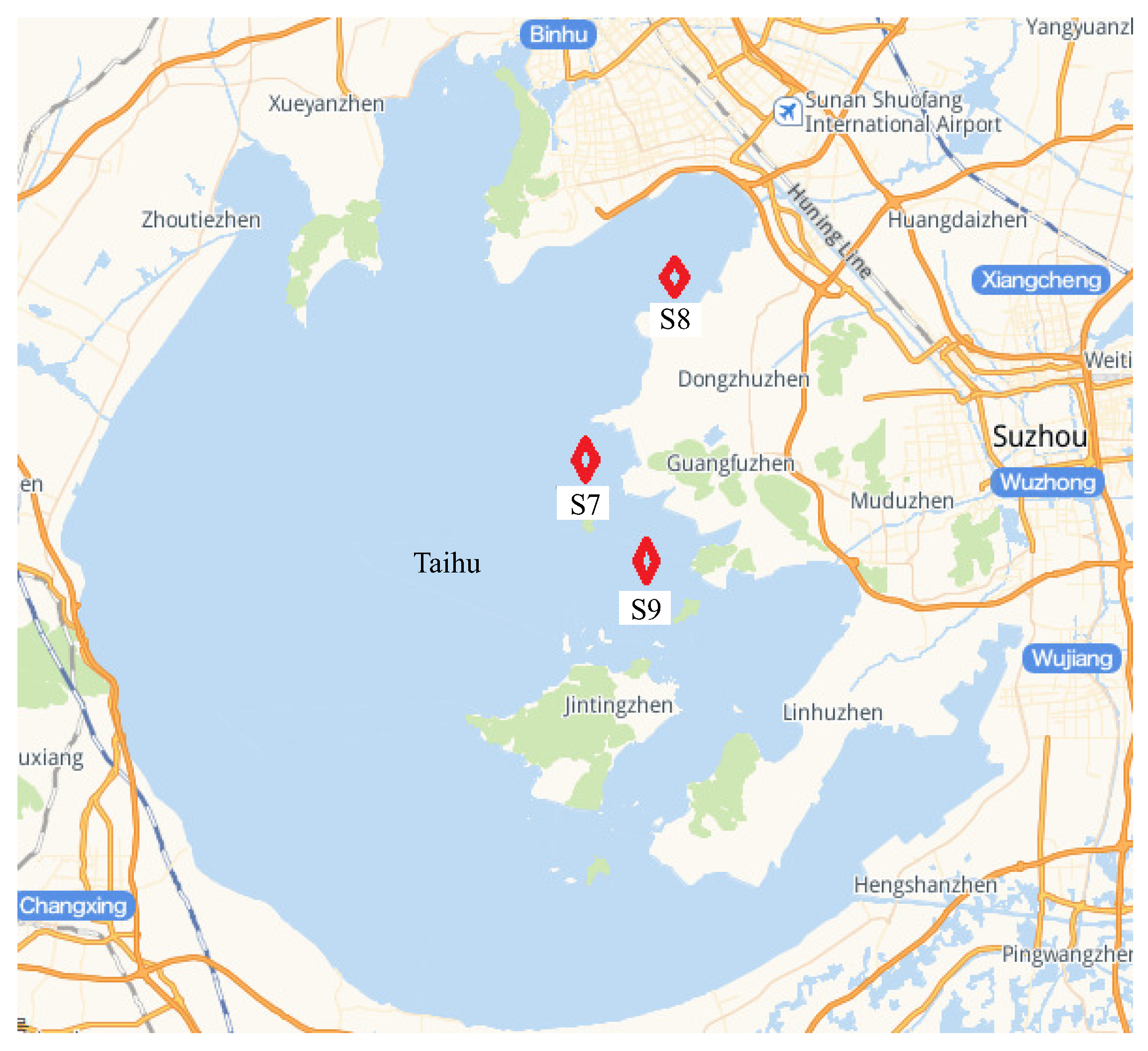
2.1. Research Area and Data Sources

Taihu Lake (${30}^{°}{5}^{\prime }$–${32}^{°}{8}^{\prime }$ N, ${119}^{°}{8}^{\prime }$–${121}^{°}{55}^{\prime }$ E) is one of the five largest freshwater lakes in China. The water area is 2156.16 square kilometers and the total length of the lake shoreline is 393.2 km [26]. Since 1980, eutrophication has continued to affect the water quality of Taihu Lake, owing to the large-scale increase in algal blooms due to increased nutrient abundance from rivers and agriculture, higher weather temperatures, and the influence of local wind conditions [27]. In particular, in 2007, a severe cyanobacterial pollution outbreak in Taihu Lake made the city stop the drinking water supply for several days [28]. This became the key event that prompted the Chinese authorities to address the water pollution problem in Taihu Lake.

In recent years, a large number of studies have been conducted on Taihu Lake. For example, Zhao et al. [29] studied the effects of cyanobacterial blooms on plankton diversity and composition in Taihu Lake, analyzing data from cyanobacteria, phytoplankton, and physicochemical samples collected in four seasons in 2017 and 2018. Zhang et al. [30] used a sub-pixel approach (algae pixel-growing algorithm) with 13 years of Moderate Resolution Imaging Spectroradiometer (MODIS) data to assess changes in bloom extension, start date, duration, and frequency of occurrence before and after a large-scale bloom event. These works introduced above provide a foundation for the study of the mechanism of cyanobacteria bloom.

In this paper, we took Taihu Lake as the research area and used the deep learning-based methods to predict algal bloom concentration. We considered the problem of the small amount of monitoring data in some waters and adopted transfer learning to learn the knowledge of algal bloom growth from waters with abundant data to improve the prediction accuracy of cyanobacterial blooms in water areas with less data.

In this paper, continuous monitoring data from the 7th, 8th, and 9th monitoring platforms in Taihu Lake were used as experimental data. The geographical location of each site is shown in Figure 1, which is marked as S7, S8, and S9 respectively. The sampling interval of the monitoring data was half an hour, and the monitoring elements of each data set included chlorophyll-a concentration (Chl-a, $\mathsf{\mu }$g/L), water temperature (Temp, °C), pH, conductivity (Conduct, $\mathsf{\mu }$S/cm), turbidity (Turb, NTU), dissolved oxygen (DO, mg/L), and cyanobacterial density (Cyanob, ${10}^4$ cells/L). These monitoring elements are often used to study the growth of algal blooms in the shallow eutrophic lakes [31].

In the experiments of this paper, S7 and S8 were used as the target domains, and S9 was used as the source domain. The selected data of S9 are from 11 June 2016, 2:00 to 30 September 2016, 24:00 with 5372 sets of data. To show the examples of the data in these monitoring platforms, some of the data in S9 are listed in

Table 1. Some of the data obtained from S9 station.

Data	Chl-a	Temp	pH	Conduct	Turb	DO	Cyanob
	($\mathsf{\mu }$g/L)	(°C)		($\mathsf{\mu }$S/cm)	(NTU)	(mg/L)	(${10}^4$ cells/L)
11 June 2016, 2:00	7.0	25.13	8.61	400	52.2	8.41	780.8
11 June 2016, 2:30	5.5	25.04	8.55	402	52.2	8.24	337.0
11 June 2016, 3:00	5.9	25.04	8.53	402	50.7	8.25	382.0
…	…	…	…	…	…	…	…
30 September 2016, 22:30	8.8	23.42	8.24	227	98.0	8.13	799.6
30 September 2016, 23:00	8.3	23.40	8.22	275	88.1	8.10	747.3
30 September 2016, 23:30	8.8	23.39	8.22	275	92.4	8.09	705.8

.

Remark 1.

Some studies indicate that there is a strong positive correlation between phytoplankton color index and chlorophyll-a estimates [32]. Thus, the chlorophyll-a concentration is often used as a surrogate indicator for the growth of cyanobacterial harmful algal blooms [15,33]. Therefore, the chlorophyll-a concentration is predicted to show the condition of the algal bloom concentration in this paper.

2.2. Proposed Method

There are very complex relationships among the influence factors of the algal blooms, including the weather and the season changes. This is the main reason why the deep-learning-based method is used in this study. The problem we study in this paper is a classical problem of multivariate time series forecasting [34,35]. The prediction process of the time series is as follows [36]: create a sliding window, and there are n data points in the window, where n is called the window size; use the n data points in the window to predict the $(n+\tau )$-th data point of the time series, where $\tau$ is called the prediction time step; slide the window along the time series to the next data point, and repeat the process above until all of the data are used.

The main idea of the proposed method is to combine the transfer learning method with deep learning method to build a fusion prediction model, which mainly includes bi-directional long short-term memory (BiLSTM), convolutional neural network (CNN), and transfer learning methods. The framework of the proposed method is shown in Figure 2, which will be introduced in details as follows.

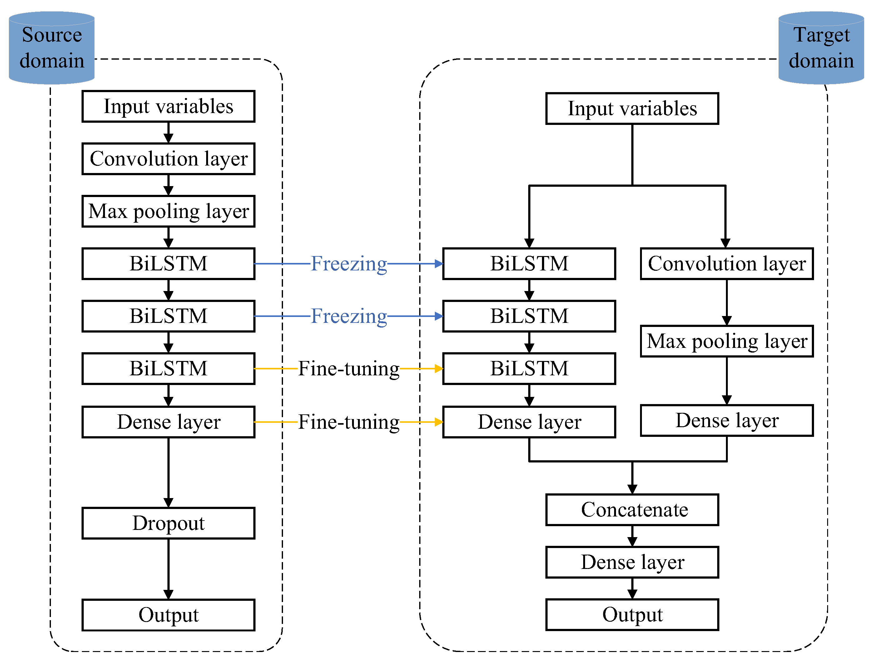
2.2.1. Transfer Learning Method for Modeling

Traditional machine learning approaches require a one-to-one relationship between the training set of data and individual models. Supervised learning with an excellent performance requires a large number of data labels for training, but many collected data in practical applications are unlabeled, and the manual labeling process is time-consuming and costly. Transfer learning is used to solve the problem of insufficient training data, which aims to apply the knowledge learned in one task to another different but similar task to improve the efficiency of solving that task. Thus, transfer learning can efficiently use existing data resources for modeling and reduce the amount of data required for new task development.

Transfer learning is divided into two categories—homogeneous and heterogeneous transfer learning [37]—and there are four main approaches for transfer learning, namely instance-based, feature-based, parameter-based, and relation-based methods [38,39]. In this study, the parameter-based transfer learning method was used for modeling. The main reason is that the parameter-based transfer methods use the model parameters learned in the source domain for the target domain, which is popular for its good compatibility with deep learning method. The details of the parameter-based transfer learning process is shown in Figure 2, which will be introduced as follows.

Domain and task are the two basic concepts of transfer learning [40]. The domain is denoted by:

$$D=\left(\pi ,P\left(X\right)\right)$$

(1)

where $\pi$ is an n-dimensional feature space, and $\pi =\left\{f_1,f_2,f_3,\cdots ,f_n\right\}$, where $f_k$ is the input feature; $X=\left\{x_1,x_2,x_3,\cdots ,x_n\right\}ϵ\pi$ is the training sample; and $P\left(X\right)$ is the marginal probability distribution of X.

Two domains with different feature spaces or unequal marginal probability distributions are considered as two different domains. In transfer learning, the domain where knowledge is acquired by learning from a large amount of data is called the source domain $D_s$, and the domain where the new task needs to be conducted by transfer learning is called the target domain $D_t$. In this paper, the task is to build a model for predicting cyanobacterial bloom concentrations of the target domain, which is defined as following:

$$M=\left(\Im ,f\left(g\right)\right)$$

(2)

where ℑ is the sequence value of the cyanobacterial bloom concentration to be predicted, and $f\left(g\right)$ is the function used to predict the task in the target domain, and can also be written as a conditional probability distribution $P\left(Y_s\left|X_s\right.\right)$, which can be learned from $\left\{x_i,y_i\right\},x_iϵX,y_iϵY$, and $Y=\left\{y_1,y_2,y_3,\cdots ,y_n\right\}ϵ\Im$.

The general workflow of transfer learning used in this paper is summarized as follows: given a source domain $D_s$ and a source task $T_s$, a target domain $D_t$, and a target task $T_t$, the purpose of transfer learning is to use the knowledge in $D_s$ and $T_s$ to train the target prediction function in the target domain $D_t$, namely the conditional distribution probabilities.

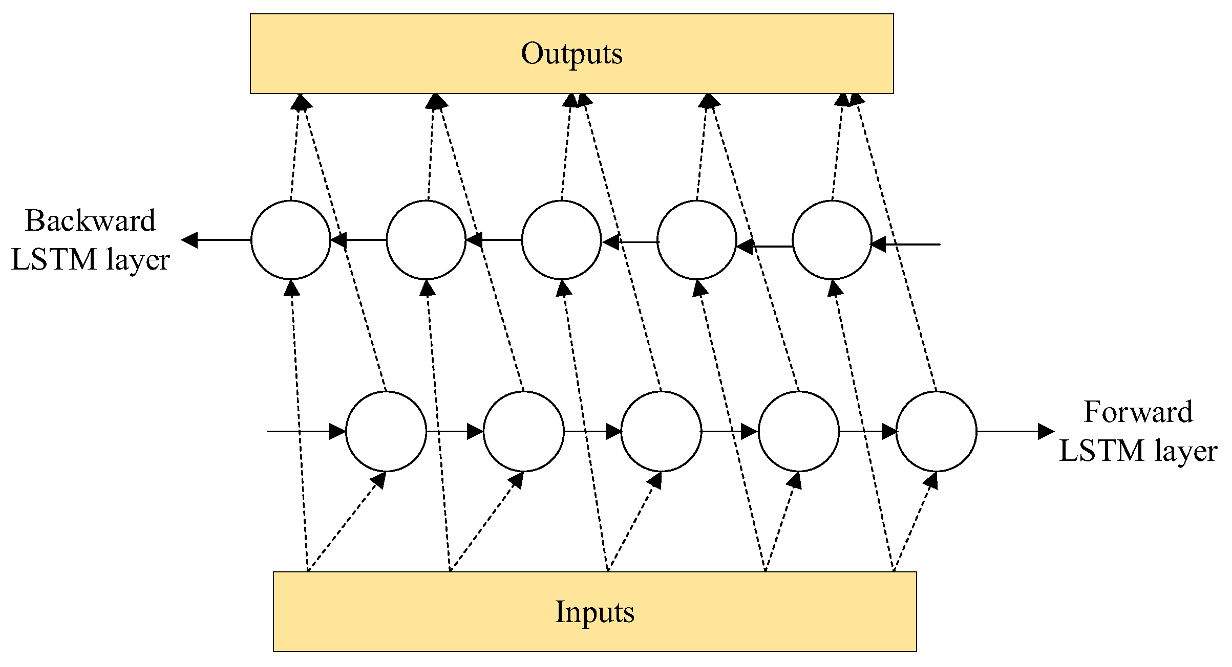
2.2.2. Feature Extraction and Time Series Prediction

In this paper, the CNN layer was used to extract features, which has unique advantages in feature extraction [41,42]. The local receptive field and weight sharing of the CNN network make the model parameters considerably lower and easier to train. Each convolutional layer contains multiple convolutional kernels, and the convolutional kernels are calculated by:

$$l_t=\delta (g_t\ast k_t+b_t)$$

(3)

where $g_t$ and $l_t$ are the input and output, respectively; $b_t$ is a bias vector; $\delta \left(·\right)$ denotes the nonlinear activation function of the convolution operation; * is the convolution operation; and $k_t$ is the weight of the convolution kernel. After the CNN layer, a pooling layer compresses the high-dimensional features extracted from the convolutional layer, which simplifies the output of the convolutional layer and improves the computational efficiency.

When the features are extracted, a bidirectional LSTM network (BiLSTM) is used for time series prediction [43], which is shown in Figure 3. In this BiLSTM network, the first input sequence is a data sample and the second is an inverted copy of the input sequence, which is passed forward and backward on the unfolded network. The main reason for using this BiLSTM structure is that the error of the traditional LSTM will become larger and larger over time [44]. The bidirectional structure increases the dependence of the data, and the prediction results are jointly determined by a number of prior and subsequent inputs, which means that the complete prior and future information of each point of the input sequence is provided to the output layer [45]. Then, the prediction results can be obtained with higher accuracy.

As shown in Figure 3, the calculation method of the backward LSTM layer is similar to the forward LSTM layer. The details of a single LSTM layer are introduced as follows [46,47]:

$$f_t=\sigma \left(W_f\left[h_{t-1}:x_t\right]+b_f\right)$$

(4)

$$o_t=\sigma \left(W_o\left[h_{t-1}:x_t\right]+b_o\right)$$

(5)

$$h_t=o_t\otimes \tanh \left(c_t\right)$$

(6)

where $f_t$ is the output of the forget gate; $W_f$ is the weight of the forget gate; $h_{t-1}$ is the hidden state of the previous LSTM cell; $x_t$ indicates the input value; $b_f$ is a bias term for the forget gate; $\left[h_{t-1}:x_t\right]$ indicates connecting the two elements; $\sigma$ indicates a sigmoid function; $o_t$ is the output of the output gate; $W_o$ and $b_o$ are the weights and biases of the output gate, respectively; $c_t$ is the update of a unit status; and ⊗ denotes the multiplication of matrix elements. All of the weights and biases are parameters that the network needs to learn. Then, the final output of BiLSTM network H can be presented by:

$$H=h_f\oplus h_b$$

(7)

where ⊕ represents the bounded plus operation of the forward LSTM layer result and the backward LSTM layer result; $h_f$ and $h_b$ are the output value of the forward LSTM network and the backward LSTM network, respectively.

2.2.3. Workflow of the Proposed Method

The training process of the model is as follows: sufficient source domain data are preprocessed, and the spatial features of the inputs among the monitoring stations are extracted by the CNN network, such as the relationship between cyanobacterial bloom concentration and other monitored water quality data. Then, these features are used as the input of BiLSTM in the next step to extract the long-term time dependence for prediction by BiLSTM. Based on the pre-training of the BiLSTM, the source domain model is obtained, which is called the original model.

In this study, a total of three layers of BiLSTM were used in the original model. When the original model was obtained, the parameters in the first two BiLSTM layers were frozen. Then, the parameters of the third BiLSTM layer and the dense layer were fine-tuned with the training set of the target domain. Based on this process, we can achieve the purpose of transferring and fusing the knowledge from the source domain to the target domain. The model that is finally obtained is called the target domain fine-tuning model.

In order to obtain better results for the prediction of the target domain, we built different sub-models to connect their results and added differences between sub-models to obtain the effects of the integration learning, and to improve the generalization ability of the prediction model. In this study, we adopted a structure with two branches (see Figure 2) in the target domain learning. One branch uses the CNN for feature extraction of the target domain’s own features, while another branch is the fine-tuned model of the target domain obtained above. Then, the outputs of the two branches were connected together by a connection layer. The dropout layer was added to solve the overfitting problem caused by too little data in the target domain. The parameters of the proposed model are listed in

Table 2. Parameter settings for each network layer of the proposed model.

Parameters	Value
Convolution layer filters	32
Convolution layer kernel size	3
Pooling layer pool size	2
BiLSTM_layer1 units	16
BiLSTM_layer2 units	32
BiLSTM_layer3 units	64
Activation function	RELU
Dropout	0.5

.

The workflow of the proposed method is summarized as follows:

Step 1: After pre-processing the data of source domain, important features and spatial correlation of sample time series are extracted through the CNN network.

Step 2: The output of the CNN network is input into 3 BiLSTM layers to obtain sequence features and long-term dependence for prediction.

Step 3: The model output is obtained through the full connection layer and the source domain model is obtained.

Step 4: The first two BiLSTM layers are frozen in the source domain model and the training data of the target domain for BiLSTM of the third layer are fine-tuned.

Step 5: The fully connected layer is used to obtain the fine-tuned model of the target domain.

Step 6: The test data of the target domain are input into both the fine-tuning model branch of the target domain and the CNN branch to extract data features.

Step 7: The outputs of the two branches of Step 6 are linked through a concatenate layer to obtain the final prediction result.

The information flow of the proposed model is shown in Figure 4.

3. Experiments and Discussion

3.1. Evaluation Criteria

To evaluate the performance of the proposed cyanobacterial bloom prediction model based on the transfer learning, the following criteria are used: mean absolute error (MAE), root mean square error (RMSE), mean square error (MSE), mean absolute percent error (MAPE), and coefficient of determination $R^2$. These evaluation metrics are often used to evaluate the performance of the deep-learning-based prediction methods [48,49], which are introduced as follows.

(1) MAE

$$\mathrm{MAE}=\frac{1}{n}\sum _{i=1}^n\left|{\widehat{y}}_i-y_i\right|$$

(8)

where n is the size of the sample, $y_i$ is the i-th true measurement, and ${\widehat{y}}_i$ is the i-th predicted value. MAE evaluates the difference between the true measurements and the predicted values.

(2) MSE and RMSE

$$\mathrm{MSE}=\frac{1}{n}\sum _{i=1}^n{\left({\widehat{y}}_i-y_i\right)}^2$$

(9)

$$\mathrm{RMSE}=\sqrt{\frac{1}{n}\sum _{i=1}^n{\left({\widehat{y}}_i-y_i\right)}^2}$$

(10)

MSE and RMSE also reflect the dispersion of the model. However, they are sensitive to large errors compared to MAE because the large errors are further magnified.

(3) MAPE

$$\mathrm{MAPE}=\frac{1}{n}\sum _{i=1}^n\frac{\left|{\widehat{y}}_i-y_i\right|}{y_i}\times 100$$

(11)

MAPE is the ratio between the error and the actual value. It can be considered as a relative error function. Small inaccuracies during periods of low-concentration cyanobacterial blooms may have a large impact on this function.

(4) $R^2$

$$R^2=1-\frac{{\sum }_{i=1}^n{\left({\widehat{y}}_i-y_i\right)}^2}{{\sum }_{i=1}^n{\left({\overline{y}}_i-y_i\right)}^2}$$

(12)

$R^2$ is used statistically to indicate the goodness-of-fit of a model.

Remark 2.

Regarding the error metrics MAE, RMSE, and MAPE, the smaller their values are, the smaller the error in the prediction results and the better the prediction performance of the model [24]. $R^2$ is used to assess the degree of conformity between the predicted and actual values. The closer it is to 1, the better the predicted and actual values match and the better the model is [50,51].

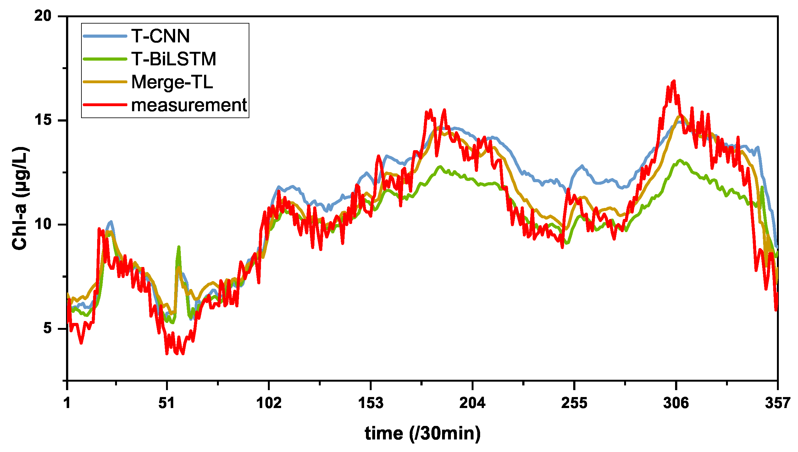
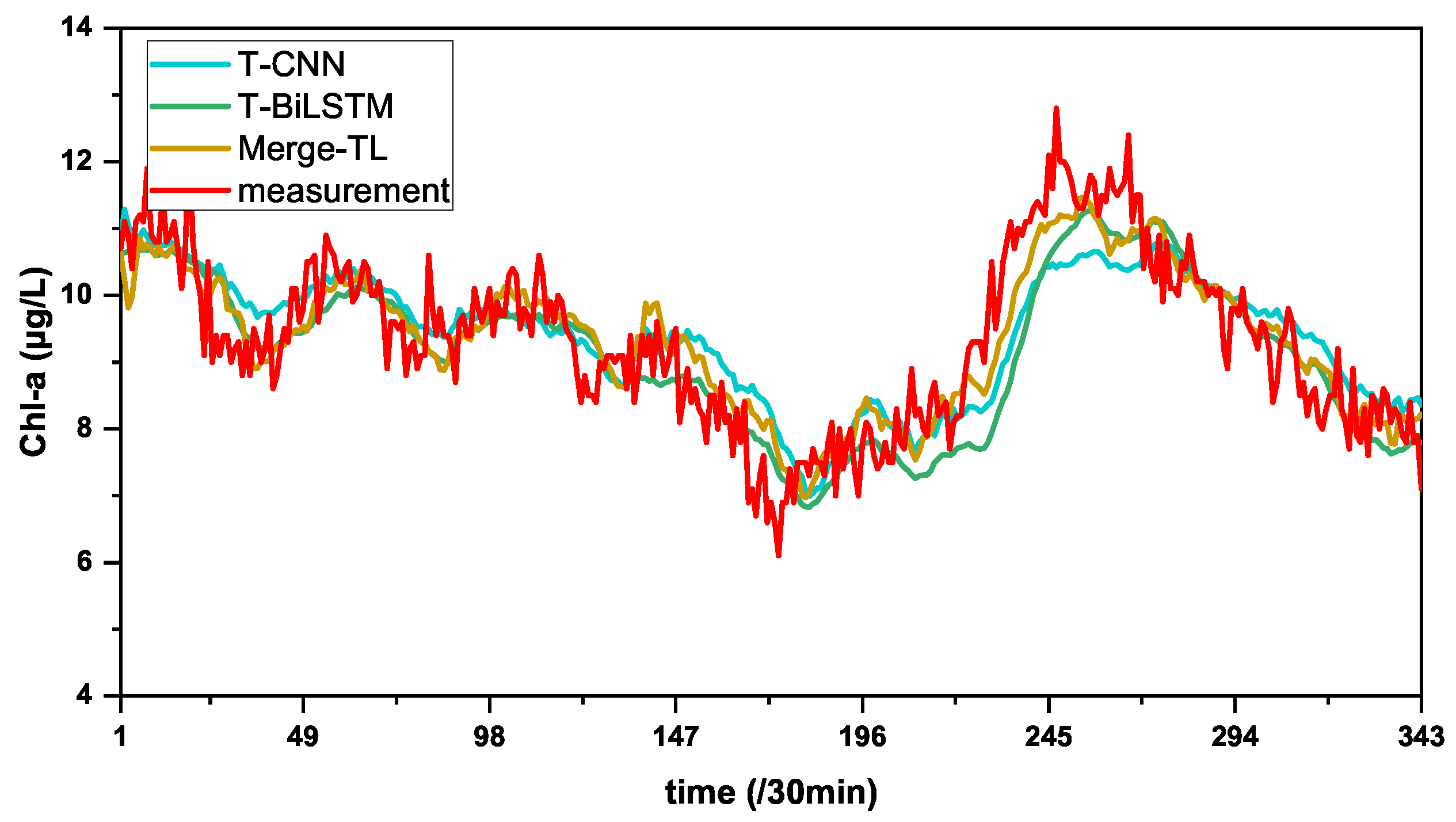
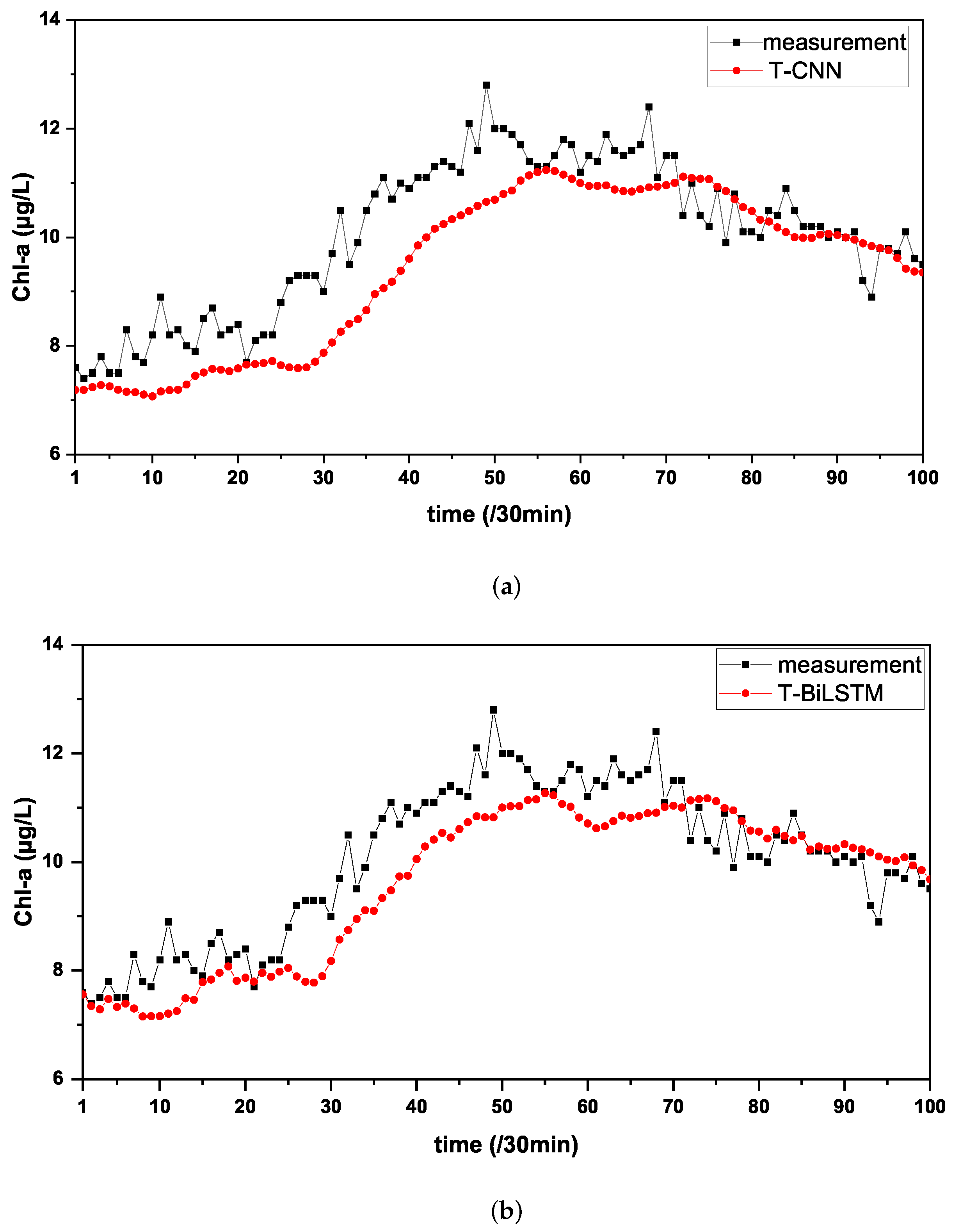
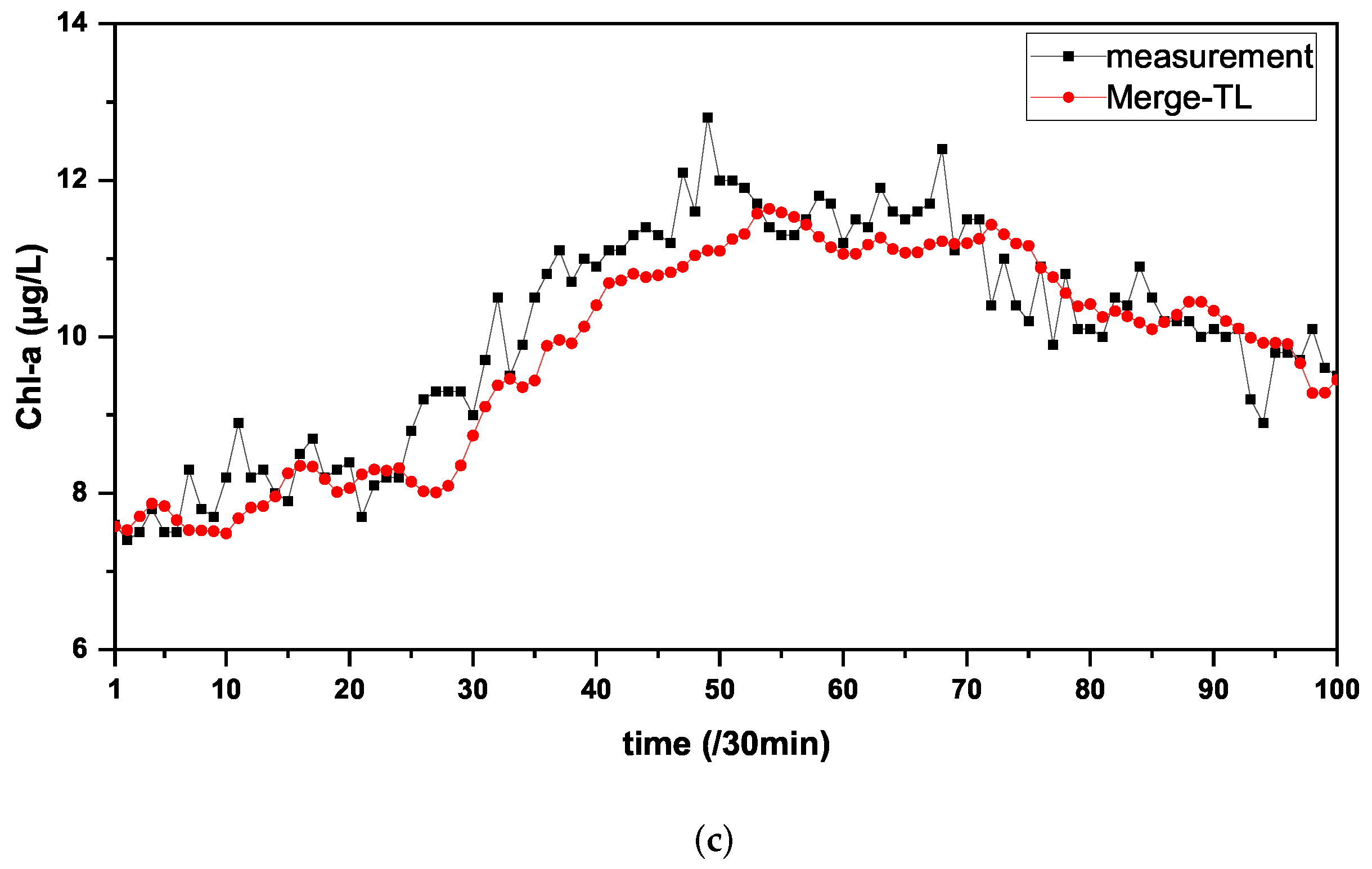
3.2. Comparison Experiment

In this experiment, the task is to predict four time steps backward (namely a 2 h prediction when the sampling interval is half an hour) of the chlorophyll-a concentration for the target domain S7. To demonstrate the performance of the proposed method, the following comparison experiments are conducted: target domain CNN model (T-CNN) prediction experiment, target domain BiLSTM model (T-BiLSTM) prediction experiment, and the proposed domain fusion transfer learning model (Merge-TL) prediction experiment. Each model is set with appropriate hyperparameters to produce the best performance. All of the models are trained using error back propagation. The neural network training process uses the Adam optimizer [52] and the MAE loss function. The batch size is set as 128; the learning rate is set as 0.001; the upper limit of the training period is set as 100, and the window size is 12. The selected data of S7 are from 1 September 2016, 0:00 to 30 September 2016, 24:00 with 1440 sets of data. The first 75% of the data sets in both the source and target domains are used as the training set and the last 25% are used as the test set. The results of each experiment are shown in

Table 3. The comparison experimental results of the 2 h prediction for S7.

Methods	MAE	RMSE	MSE	MAPE	${\mathit{R}}^2$
T-CNN	0.5292	0.6628	0.4393	5.7125	0.7343
T-BiLSTM	0.5048	0.6373	0.4062	5.3544	0.7545
Merge-TL	0.4336	0.5589	0.3124	4.7179	0.8110

.

From the results in Table 3, it can be seen that the proposed model performs better than the traditional model in all evaluation indexes, with the MAE decreasing by 18.07% compared to T-CNN and 14.10% compared to T-BiLSTM; the RMSE decreasing by 15.67% and 12.30% compared to T-CNN and T-BiLSTM, respectively; and the MAPE declining by 17.41% and 11.89%, respectively.

In this experiment, a total of 345 data points were predicted. To show the superior performance of the proposed model more visually, we selected 100 data points with relatively large changes in the chlorophyll-a concentration for visualization, and the results are shown in Figure 5. The time period corresponding to these 100 data points is from 23:30 on 27 September to 1:00 on 30 September. From the curves of Figure 5, we can see that the prediction value based on the proposed model is most close to the real value.

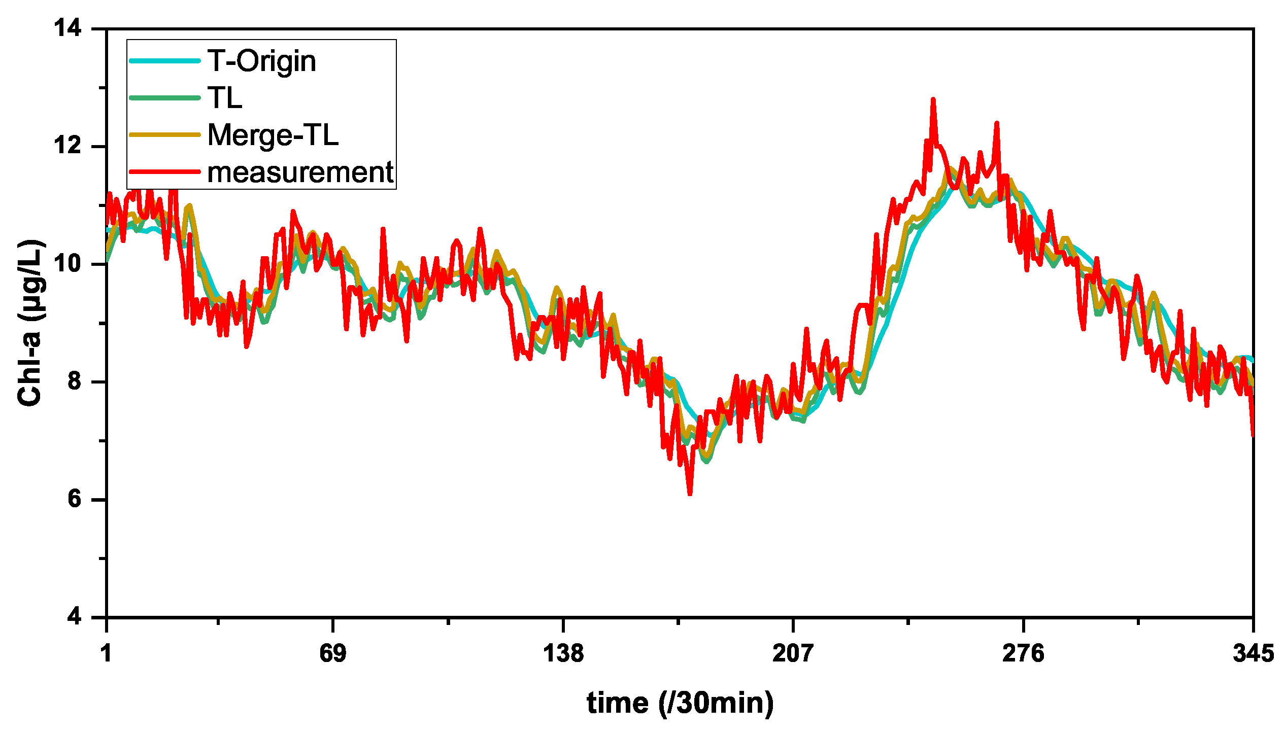
3.3. Ablation Experiments

To demonstrate the effectiveness of the proposed model, we also performed two ablation experiments: one is the target domain original model (T-Origin) prediction experiment, and the other is the direct transfer model (TL) prediction experiment. The T-Origin model has the same structure as the source domain training model (see Figure 2), and the TL model is the same as the proposed model, but without adding CNN branches for fusion. The results of the ablation experiments are shown in

Table 4. The ablation experimental results of the 2 h prediction for S7.

Methods	MAE	RMSE	MSE	MAPE	${\mathit{R}}^2$
T-Origin	0.4814	0.6216	0.3864	5.2147	0.7662
TL	0.4470	0.5749	0.3305	4.7871	0.8000
Merge-TL	0.4336	0.5589	0.3124	4.7179	0.8110

. The performance of each model for the ablation experiments is shown in Figure 6, where the total number of the prediction data points is 345 and the corresponding time period is from 19:30 on 23 September to 23:30 on 30 September.

The MAE, RMSE, MSE, and MAPE for the Merge-TL models are all the smallest, with each value decreasing by 9.93%, 10.09%, 19.15%, and 9.53%, respectively, compared to the T-Origin model, and each value decreasing by 3.00%, 2.78%, 5.48%, and 1.45%, respectively, compared to the TL model. The value of $R^2$ for the Merge-TL model increased by 5.85% over the T-Origin model and 1.38% over the TL model. The results of these ablation experiments show that the improvements of the proposed model are very important to improve the accuracy of chlorophyll concentration prediction.

3.4. Discussion

The results of the comparison experiments in Section 3.2 show that the proposed model has a better performance than that of the state-of-the-art. To further analyze the performance of the proposed model, some expanded discussions about other key issues on the cyanobacterial bloom prediction model are given out in this section, including the generalization ability and the prediction time.

3.4.1. About the Generalization

The generalization performance of a model is a measurement of the performance of the model on datasets outside of the training samples [53]. In this study, to validate the generalization ability of the proposed model, we used another monitoring station, S8, as the target domain. The data of the target domain S8 are selected from August 2016 with 1488 sets of data. The source domain is still S9 and its data are the same as those used in Section 3.2. In this experiment, the first $75\%$ of the data sets in both the source and target domains are used as the training set and the last $25\%$ are used as the test set. The prediction results of each model are shown in

Table 5. Results of the 2 h prediction for the site S8.

Methods	MAE	RMSE	MSE	MAPE	${\mathit{R}}^2$
T-CNN	1.2492	1.6564	2.7436	14.2893	0.7107
T-BiLSTM	1.1205	1.5214	2.3145	11.5404	0.7560
Merge-TL	1.0108	1.3572	1.8298	12.0023	0.8061

. The results in Table 5 show that the proposed model is superior to other models in four evaluation indexes, except the MAPE. The prediction results of each model are shown in Figure 7, where the total number of the prediction data points is 357 and the corresponding time period is from 13:30 on 24 August to 23:30 on 31 August. It can be seen that the proposed model can track the changing trend of chlorophyll-a concentration well.

3.4.2. About the Prediction Time

The discussion of the prediction time concerns testing the robustness of the proposed model. In this study, to further verify the performance of the model for a longer prediction time, we used S7 as the target domain to conduct 3 h (six time steps) prediction experiments on the T-CNN model, T-BiLSTM model and Merge-TL model, respectively. The results are shown in

Table 6. Results of the 3 h prediction for site S7.

Methods	MAE	RMSE	MSE	MAPE	${\mathit{R}}^2$
T-CNN	0.5761	0.7401	0.5477	6.2951	0.6676
T-BiLSTM	0.5279	0.7003	0.4904	5.6461	0.7024
Merge-TL	0.4679	0.5933	0.3520	5.1302	0.7863

and Figure 8. When the prediction time is 3 h, there are a total of 343 data points to be predicted, and the corresponding time period is from 20:30 on September 23 to 23:30 on September 30. According to the five evaluation indexes in Table 6, the proposed model has a better performance when the prediction periods are prolonged. The visualizations of the 3 h prediction results of each model in Figure 8 show that the proposed model can predict the change in the chlorophyll-a concentration well at relatively longer prediction periods.

4. Conclusions

In this paper, deep learning and transfer learning techniques are applied to the prediction of cyanobacterial bloom concentration time series in aquatic systems, and a fused transfer learning model is proposed to transfer knowledge from waters with abundant water quality monitoring data to waters with insufficient water quality monitoring data to achieve the cross-water prediction of the cyanobacterial bloom concentration. Transfer learning has some benefits in improving the model performance. The potential practical value of this work is that we can save the amount of monitoring data collected and, for waters with inconvenient geographic locations, the number of sensors used, saving manpower and material resources. However, there are some limitations of the proposed model, which is a single-source domain transfer learning model that has a relatively short forecast time period. These problems should be further studied.

The research data in this paper are all from various stations in Taihu Lake, so, in future work, we will investigate whether the model can cover a wider area, which would be very meaningful if feasible. In addition, we will consider building a fusion model of deep learning and transfer learning to combine remote sensing images to predict cyanobacterial bloom concentration sequences in order to achieve a better prediction accuracy.

References

1. Ndlela, L.L.; Oberholster, P.J.; Van Wyk, J.H.; Cheng, P.H. An overview of cyanobacterial bloom occurrences and research in Africa over the last decade. Harmful Algae 2016, 60, 11–26. [Google Scholar] [CrossRef] [PubMed]
2. Huo, D.; Gan, N.; Geng, R.; Cao, Q.; Song, L.; Yu, G.; Li, R. Cyanobacterial blooms in China: Diversity, distribution, and cyanotoxins. Harmful Algae 2021, 109, 102106. [Google Scholar] [CrossRef] [PubMed]
3. Best, J.; Eddy, F.; Codd, G. Effects of Microcystis cells, cell extracts and lipopolysaccharide on drinking and liver function in rainbow trout Oncorhynchus mykiss Walbaum. Aquat. Toxicol. 2003, 64, 419–426. [Google Scholar] [CrossRef]
4. Meng, G.; Sun, Y.; Fu, W.; Guo, Z.; Xu, L. Microcystin-LR induces cytoskeleton system reorganization through hyperphosphorylation of tau and HSP27 via PP2A inhibition and subsequent activation of the p38 MAPK signaling pathway in neuroendocrine (PC12) cells. Toxicology 2011, 290, 218–229. [Google Scholar] [CrossRef] [PubMed]
5. Chen, L.; Chen, J.; Zhang, X.; Xie, P. A review of reproductive toxicity of microcystins. J. Hazard. Mater. 2016, 301, 381–399. [Google Scholar] [CrossRef] [PubMed]
6. Yan, T.; Li, X.D.; Tan, Z.J.; Yu, R.C.; Zou, J.Z. Toxic effects, mechanisms, and ecological impacts of harmful algal blooms in China. Harmful Algae 2022, 111, 102148. [Google Scholar] [CrossRef] [PubMed]
7. Aguilera, A.; Haakonsson, S.; Martin, M.V.; Salerno, G.L.; Echenique, R.O. Bloom-forming cyanobacteria and cyanotoxins in Argentina: A growing health and environmental concern. Limnologica 2018, 69, 103–114. [Google Scholar] [CrossRef]
8. Gorham, T.; Dowling Root, E.; Jia, Y.; Shum, C.; Lee, J. Relationship between cyanobacterial bloom impacted drinking water sources and hepatocellular carcinoma incidence rates. Harmful Algae 2020, 95, 101801. [Google Scholar] [CrossRef]
9. Xia, R.; Zhang, Y.; Wang, G.; Zhang, Y.; Dou, M.; Hou, X.; Qiao, Y.; Wang, Q.; Yang, Z. Multi-factor identification and modelling analyses for managing large river algal blooms. Environ. Pollut. 2019, 254, 113056. [Google Scholar] [CrossRef]
10. Ranjbar, M.H.; Hamilton, D.P.; Etemad-Shahidi, A.; Helfer, F. Individual-based modelling of cyanobacteria blooms: Physical and physiological processes. Sci. Total Environ. 2021, 792, 148418. [Google Scholar] [CrossRef]
11. Havens, K.E.; James, R.T.; East, T.L.; Smith, V.H. N:P ratios, light limitation, and cyanobacterial dominance in a subtropical lake impacted by non-point source nutrient pollution. Environ. Pollut. 2003, 122, 379–390. [Google Scholar] [CrossRef]
12. Xu, T.; Yang, T.; Zheng, X.; Li, Z.; Qin, Y. Growth limitation status and its role in interpreting chlorophyll a response in large and shallow lakes: A case study in Lake Okeechobee. J. Environ. Manag. 2022, 302, 114071. [Google Scholar] [CrossRef] [PubMed]
13. Menshutkin, V.; Astrakhantsev, G.; Yegorova, N.; Rukhovets, L.; Simo, T.; Petrova, N. Mathematical modeling of the evolution and current conditions of the Ladoga Lake ecosystem. Ecol. Model. 1998, 107, 1–24. [Google Scholar] [CrossRef]
14. Muhammetoglu, A.; Soyupak, S. A three-dimensional water quality-macrophyte interaction model for shallow lakes. Ecol. Model. 2000, 133, 161–180. [Google Scholar] [CrossRef]
15. Lee, S.; Lee, D. Improved Prediction of Harmful Algal Blooms in Four Major South Korea’s Rivers Using Deep Learning Models. Int. J. Environ. Res. Public Health 2018, 15, 1322. [Google Scholar] [CrossRef] [Green Version]
16. Ni, J.; Shen, K.; Chen, Y.; Cao, W.; Yang, S.X. An Improved Deep Network-Based Scene Classification Method for Self-Driving Cars. IEEE Trans. Instrum. Meas. 2022, 71, 5001614. [Google Scholar] [CrossRef]
17. Son, H.; Lee, B.; Sung, S. Synthetic Deep Neural Network Design for Lidar-inertial Odometry Based on CNN and LSTM. Int. J. Control. Autom. Syst. 2021, 19, 2859–2868. [Google Scholar] [CrossRef]
18. Mutabazi, E.; Ni, J.; Tang, G.; Cao, W. A Review on Medical Textual Question Answering Systems Based on Deep Learning Approaches. Appl. Sci. 2021, 11, 5456. [Google Scholar] [CrossRef]
19. Recknagel, F. ANNA—Artificial Neural Network model for predicting species abundance and succession of blue-green algae. Hydrobiologia 1997, 349, 47–57. [Google Scholar] [CrossRef]
20. Hill, P.R.; Kumar, A.; Temimi, M.; Bull, D.R. HABNet: Machine Learning, Remote Sensing-Based Detection of Harmful Algal Blooms. IEEE J. Sel. Top. Appl. Earth Obs. Remote Sens. 2020, 13, 3229–3239. [Google Scholar] [CrossRef]
21. Cho, H.; Choi, U.; Park, H. Deep learning application to time-series prediction of daily chlorophyll-a concentration. WIT Trans. Ecol. Environ. 2018, 215, 157–163. [Google Scholar]
22. Wu, D.; Wang, X.; Wu, S. Jointly modeling transfer learning of industrial chain information and deep learning for stock prediction. Expert Syst. Appl. 2022, 191, 116257. [Google Scholar] [CrossRef]
23. Grubinger, T.; Chasparis, G.C.; Natschlager, T. Generalized online transfer learning for climate control in residential buildings. Energy Build. 2017, 139, 63–71. [Google Scholar] [CrossRef] [Green Version]
24. Hu, Q.; Zhang, R.; Zhou, Y. Transfer learning for short-term wind speed prediction with deep neural networks. Renew. Energy 2016, 85, 83–95. [Google Scholar] [CrossRef]
25. Tian, W.; Liao, Z.; Wang, X. Transfer learning for neural network model in chlorophyll-a dynamics prediction. Environ. Sci. Pollut. Res. 2019, 26, 29857–29871. [Google Scholar] [CrossRef] [PubMed]
26. Cao, H.; Han, L.; Li, L. A deep learning method for cyanobacterial harmful algae blooms prediction in Taihu Lake, China. Harmful Algae 2022, 113, 102189. [Google Scholar] [CrossRef]
27. Huang, J.; Cui, Z.; Tian, F.; Huang, Q.; Gao, J.; Wang, X.; Li, J. Modeling nitrogen export from 2539 lowland artificial watersheds in Lake Taihu Basin, China: Insights from process-based modeling. J. Hydrol. 2020, 581, 124428. [Google Scholar] [CrossRef]
28. Liu, Y.; Chen, W.; Li, D.; Huang, Z.; Shen, Y.; Liu, Y. Cyanobacteria-/cyanotoxin-contaminations and eutrophication status before Wuxi Drinking Water Crisis in Lake Taihu, China. J. Environ. Sci. 2011, 23, 575–581. [Google Scholar] [CrossRef]
29. Zhao, K.; Wang, L.; You, Q.; Pan, Y.; Liu, T.; Zhou, Y.; Zhang, J.; Pang, W.; Wang, Q. Influence of cyanobacterial blooms and environmental variation on zooplankton and eukaryotic phytoplankton in a large, shallow, eutrophic lake in China. Sci. Total Environ. 2021, 773, 145421. [Google Scholar] [CrossRef]
30. Zhang, Y.; Ma, R.; Duan, H.; Loiselle, S.A.; Xu, J. Satellite analysis to identify changes and drivers of CyanoHABs dynamics in Lake Taihu. Water Sci. Technol. Water Supply 2016, 16, 1451–1466. [Google Scholar] [CrossRef]
31. Zou, W.; Zhu, G.; Xu, H.; Zhu, M.; Zhang, Y.; Qin, B. Temporal dependence of chlorophyll a-nutrient relationships in Lake Taihu: Drivers and management implications. J. Environ. Manag. 2022, 306, 114476. [Google Scholar] [CrossRef] [PubMed]
32. Zheng, L.; Wang, H.; Liu, C.; Zhang, S.; Ding, A.; Xie, E.; Li, J.; Wang, S. Prediction of harmful algal blooms in large water bodies using the combined EFDC and LSTM models. J. Environ. Manag. 2021, 295, 113060. [Google Scholar] [CrossRef] [PubMed]
33. Huang, J.; Xu, Q.; Wang, X.; Xi, B.; Jia, K.; Huo, S.; Liu, H.; Li, C.; Xu, B. Evaluation of a modified monod model for predicting algal dynamics in Lake Tai. Water 2015, 7, 3626–3642. [Google Scholar] [CrossRef] [Green Version]
34. Cruz, R.C.; Reis Costa, P.; Vinga, S.; Krippahl, L.; Lopes, M.B. A Review of Recent Machine Learning Advances for Forecasting Harmful Algal Blooms and Shellfish Contamination. J. Mar. Sci. Eng. 2021, 9, 283. [Google Scholar] [CrossRef]
35. Han, Z.; Zhao, J.; Leung, H.; Ma, K.F.; Wang, W. A Review of Deep Learning Models for Time Series Prediction. IEEE Sens. J. 2021, 21, 7833–7848. [Google Scholar] [CrossRef]
36. Ma, J.; Cheng, J.C.; Lin, C.; Tan, Y.; Zhang, J. Improving air quality prediction accuracy at larger temporal resolutions using deep learning and transfer learning techniques. Atmos. Environ. 2019, 214, 116885. [Google Scholar] [CrossRef]
37. Weiss, K.; Khoshgoftaar, T.M.; Wang, D. A Survey of Transfer Learning. J. Big Data 2016, 3, 9. [Google Scholar] [CrossRef] [Green Version]
38. Zhuang, F.; Qi, Z.; Duan, K.; Xi, D.; Zhu, Y.; Zhu, H.; Xiong, H.; He, Q. A Comprehensive Survey on Transfer Learning. Proc. IEEE 2021, 109, 43–76. [Google Scholar] [CrossRef]
39. Pan, S.J.; Yang, Q. A Survey on Transfer Learning. IEEE Trans. Knowl. Data Eng. 2010, 22, 1345–1359. [Google Scholar] [CrossRef]
40. Li, B.; Rangarajan, S. A conceptual study of transfer learning with linear models for data-driven property prediction. Comput. Chem. Eng. 2022, 157, 107599. [Google Scholar] [CrossRef]
41. Boureau, Y.L.; Bach, F.; LeCun, Y.; Ponce, J. Learning mid-level features for recognition. In Proceedings of the 2010 IEEE Computer Society Conference on Computer Vision and Pattern Recognitio, San Francisco, CA, USA, 13–18 June 2010; pp. 2559–2566. [Google Scholar]
42. Ni, J.; Chen, Y.; Chen, Y.; Zhu, J.; Ali, D.; Cao, W. A Survey on Theories and Applications for Self-Driving Cars Based on Deep Learning Methods. Appl. Sci. 2020, 10, 2749. [Google Scholar] [CrossRef]
43. Graves, A.; Schmidhuber, J. Framewise phoneme classification with bidirectional LSTM and other neural network architectures. Neural Netw. 2005, 18, 602–610. [Google Scholar] [CrossRef] [PubMed]
44. Ma, X.; Hovy, E. End-to-end Sequence Labeling via Bi-directional LSTM-CNNs-CRF. In Proceedings of the 54th Annual Meeting of the Association for Computational Linguistics, Berlin, Germany, 7–12 August 2016; pp. 1064–1074. [Google Scholar]
45. Ghasemlounia, R.; Gharehbaghi, A.; Ahmadi, F.; Saadatnejadgharahassanlou, H. Developing a novel framework for forecasting groundwater level fluctuations using Bi-directional Long Short-Term Memory (BiLSTM) deep neural network. Comput. Electron. Agric. 2021, 191, 106568. [Google Scholar] [CrossRef]
46. Shi, P.; Fang, X.; Ni, J.; Zhu, J. An Improved Attention-Based Integrated Deep Neural Network for PM2.5 Concentration Prediction. Appl. Sci. 2021, 11, 4001. [Google Scholar] [CrossRef]
47. Chen, S.; Han, X.; Shen, Y.; Ye, C. Application of Improved LSTM Algorithm in Macroeconomic Forecasting. Comput. Intell. Neurosci. 2021, 2021, 4471044. [Google Scholar] [CrossRef]
48. Bai, Y.; Liu, M.D.; Ding, L.; Ma, Y.J. Double-layer staged training echo-state networks for wind speed prediction using variational mode decomposition. Appl. Energy 2021, 301, 117461. [Google Scholar] [CrossRef]
49. Sun, W.; Xu, Z. A novel hourly PM2.5 concentration prediction model based on feature selection, training set screening, and mode decomposition-reorganization. Sustain. Cities Soc. 2021, 75, 103348. [Google Scholar] [CrossRef]
50. Rajaee, T.; Boroumand, A. Forecasting of chlorophyll-a concentrations in South San Francisco Bay using five different models. Appl. Ocean Res. 2015, 53, 208–217. [Google Scholar] [CrossRef]
51. Al Shehhi, M.R.; Kaya, A. Time series and neural network to forecast water quality parameters using satellite data. Cont. Shelf Res. 2021, 231, 104612. [Google Scholar] [CrossRef]
52. Le Guen, V.; Thome, N. Shape and Time Distortion Loss for Training Deep Time Series Forecasting Models. In Proceedings of the 33rd Annual Conference on Neural Information Processing Systems (NIPS 2019), Vancouver, BC, Canada, 8–14 December 2019. [Google Scholar]
53. LeCun, Y.; Bengio, Y.; Hinton, G. Deep Learning. Nature 2015, 521, 436–444. [Google Scholar] [CrossRef]
Figure 1. Locations of the monitoring platforms.
Water 14 01300 g001
Figure 2. The framework of the proposed method.
Water 14 01300 g002
Figure 3. The diagram of the BiLSTM structure.
Water 14 01300 g003
Figure 4. The information flow of the proposed model.
Water 14 01300 g004
Figure 5. Visualization of 100 data points for each model prediction result, where the time period of the data points is from 23:30 on 27 September to 1:00 on 30 September. (a) Results of the T-CNN prediction model. (b) Results of the T-BiLSTM prediction model. (c) Results of the Merge-TL prediction model.
Water 14 01300 g005aWater 14 01300 g005b
Figure 6. Results of the ablation experiments, where the total number of the prediction data points is 345 and the corresponding time period is from 19:30 on 23 September to 23:30 on 30 September.
Water 14 01300 g006
Figure 7. Results of the 2 h prediction for each model at the site S8, where the total number of the prediction data points is 357 and the corresponding time period is from 13:30 on 24 August to 23:30 on 31 August.
Water 14 01300 g007
Figure 8. Results of the 3 h prediction for each model at site S7, where the total number of the prediction data points is 343, and the corresponding time period is from 20:30 on 23 September to 23:30 on 30 September.
Water 14 01300 g008