Use of a Raspberry-Pi Video Camera for Coastal Flooding Vulnerability Assessment: The Case of Riccione (Italy)

Abstract

Coastal monitoring is strategic for the correct assessment of nearshore morphodynamics, to verify the effects of anthropogenic interventions for the purpose of coastal protection and for the rapid assessment of flooding vulnerability due to severe events. Remote sensing and field surveys are among the main approaches that have been developed to meet these necessities. Key parameters in the assessment and prevision of coastal flooding extensions, beside meteomarine characteristics, are the topography and slope of beaches, which can be extremely dynamic. The use of continuous monitoring through orthorectified video images allows for the rapid detection of the intertidal bathymetry and flooding threshold during severe events. The aim of this work was to present a comparison of different monitoring strategies and methodologies that have been integrated into repeated surveys in order to evaluate the performance of a new camera system. We used a low-cost camera based on Raspberry Pi called VISTAE (Video monitoring Intelligent STAtion for Environmental applications) for long-term remote observations and GNSS-laser tools for field measurements. The case study was a coastal tract in Riccione, Italy (Northern Adriatic Sea), which is the seat of nourishment interventions and of different types of underwater protection structures to combat coastal erosion. We performed data acquisition and analysis of the emerged beach and of the swash zone in terms of the intertidal bathymetry and shoreline. The results show a generally good agreement between the field and remote measurements through image processing, with a small discrepancy of the order of ≈0.05 m in the vertical and ≈1.5 m in the horizontal in terms of the root mean square error (RMSE). These values are comparable with that of current video monitoring instruments, but the VISTAE has the advantages of its low-cost, programmability and automatized analyses. This result, together with the possibility of continuous monitoring during daylight hours, supports the advantages of a combined approach in coastal flooding vulnerability assessment through integrated and complementary techniques.

1. Introduction

The characterization of flood hazard maps and of the evolution of the nearshore morphology is a fundamental factor in the evaluation of the state of a given beach and for coastal management [1,2]. For the most part, information can be derived in terms of the morphology of the emerged beach, the bathymetry and the hydrodynamics conditions of the submerged beach. In coastal monitoring, two factors should be considered to evaluate the accuracy of measurements: spatial resolution and temporal resolution [3]. Very high-resolution in space can be reached through field surveys using cutting-edge instrumentation such as GNSS (Global Navigation Satellite System) and TLS (Terrestrial Laser Scanner) [4,5]. However, it is not always possible to carry out very frequently repeated surveys, such as daily surveys, of the same beach with GNSS and/or TLS measurements, due to technical limitations, eventual adverse meteomarine conditions and high costs (surveys are time-consuming and instruments are expensive). Consequently, field campaigns are commonly repeated with seasonal frequency and therefore available at significant dates, resulting in low temporal resolution.

In order to overcome these issues and guarantee an adequate temporal coverage of the observations, other coastal monitoring methods have been developed over the last few decades [6,7,8]. Amongst other methods, measurements of coastal morphology and dynamics have been realized through remote observations, such as images from satellites [9] or video cameras installed on drones [10] or on fixed positions [11]. Remote techniques can indeed also be used during intense meteomarine events, are generally less expensive and provide a high-resolution temporal coverage if integrated with field measurements.

The use of video cameras has become more common for research on coastal processes and in support of coastal management. Many examples on the opportunities that this technology provides are available in the literature. For instance, just to give a short review, results were presented from the Coastview project in 2007 [12,13], when the potentialities of video cameras for coastal management were first the object of a European-funded project, or from recent applications with smartphones [14,15], which also show how this technology can be based on social involvement. Several interesting results have been obtained in the region of this study (Emilia-Romagna), but always with expensive systems [12,16].

The diffusion of high-resolution cameras and the development of sophisticated algorithms for image processing and segmentation also allows for the obtainment of coastal indicators (e.g., shoreline position, intertidal bathymetry, run-up) with adequate spatial accuracy and high temporal resolution. However, the choice of a suitable shoreline detection model is crucial to obtain reliable data and, ultimately, to reconstruct the intertidal bathymetry [17]. Several algorithms have been developed in recent decades. At first, methods relied on the correlation between pixel intensity on a greyscale image and wave dissipation, i.e., ShoreLine Intensity Maximum (SLIM) [18]. SLIM, however, tends to fail in the presence of emerged bars and other conditions which limit intensity-dissipation correlation on the swash zone. Consequently, other algorithms were proposed, such as Pixel Intensity Clustering (PIC) [19,20], Color Channel Difference (CCD) [21] and Artificial Neural Network-based techniques [22]. Recently, a new Shoreline Detection Model (SDM) was developed to automatically retrieve the shoreline using transformed images in CIELab color space and to avoid limitation due to the choice of the region of interest [23]. In this work, we automatically detected the shoreline through a binary image segmentation (see Section 3.1). Then, the extracted shorelines were visually observed to check the quality of the method and to modify errors. This procedure allowed us to be confident that the used technique did not affect the accuracy of the shoreline detection and, consequently, the intertidal bathymetry.

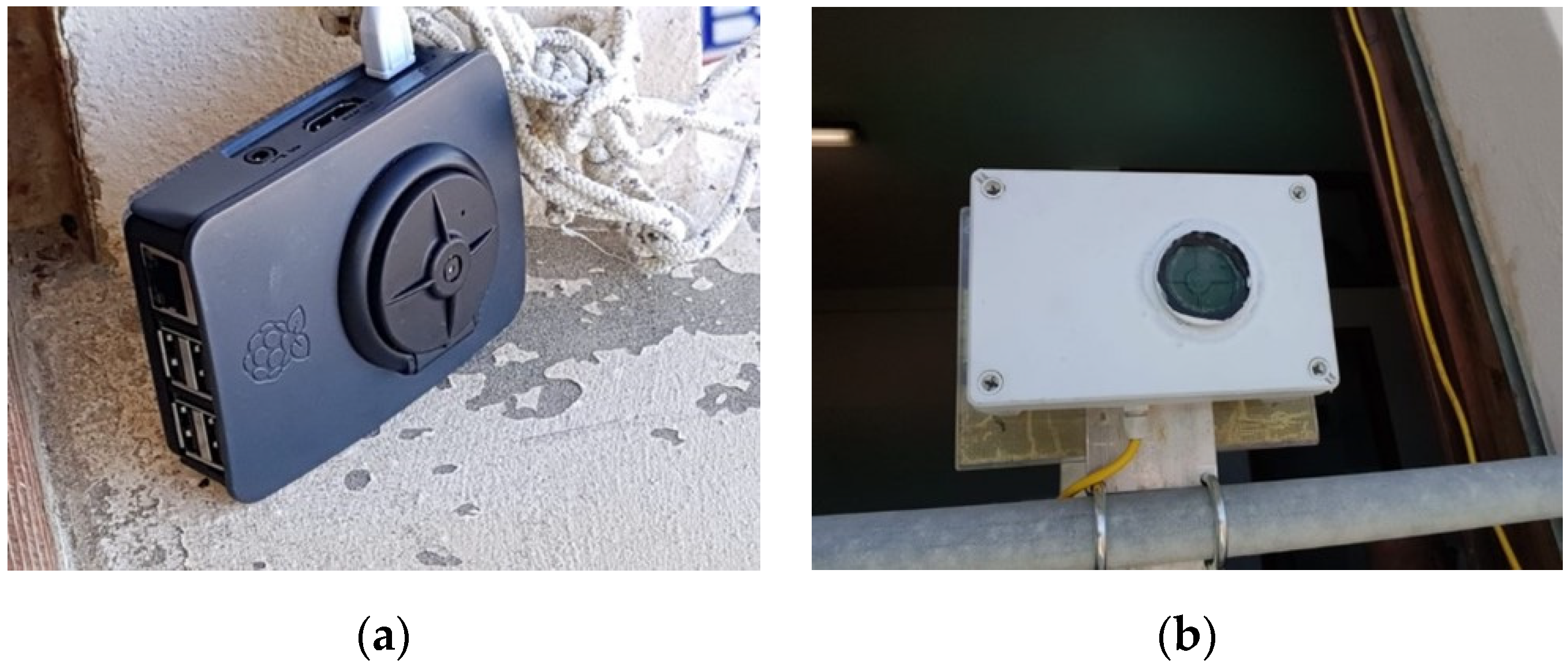
In this context, the implementation of smart and innovative low-cost cameras with the capability of autonomously performing in-situ ad-hoc analyses represents an important update. This remote data could be easily coupled with field measurements for long-term coastal monitoring; in this way, data with high temporal resolution (but less accuracy) can be complemented and validated by data with very high spatial resolution (but limited in time and in terms of the number of surveys). Guided by this objective, we have developed a novel technology which uses a small-size computer (Raspberry Pi) and a camera (Pi Camera Module v2, with a resolution up to 8 megapixels) as a smart tool to autonomously acquire and analyze images of a coastal stretch. The use of Raspberry Pi in integrated smart systems has increased exponentially in recent years. This is probably due to the potential of this camera system to produce scientific quality data, as comprehensively studied and illustrated by [24]. In marine and aquatic research, Raspberry Pi has been used as a low-cost system for underwater smart-cameras [25,26,27], for audio recorders [28] and for unmanned vehicles [29], to cite some applications. In environmental science and engineering, a Raspberry Pi system has been used to remotely check the atmospheric and temperature conditions of a fresco painting in adverse ambient conditions [30] and to observe rockfalls in surface mining environments [31].

The main advantages of applying this new tool in coastal monitoring are several: its programmability, which allows for the development of customizable analyses for each study site, the ease of its deployment thanks to its reduced size and its very low-cost. In this work, we assessed the performance of a low-cost smart camera called VISTAE coupled with periodic field surveys by using GNSS and TLS, which are fundamental to validating the results of the video and provide data with high spatial resolution of the observed coastal stretch for seasonal evaluations of the beach state.

A first attempt to use Raspberry Pi was recently performed in coastal monitoring [32], but the main goal of that study was to predict the overwash hazard on a rocky shore platform. Here, the use of a very low-cost camera is a novelty in the context of the coastal video monitoring of a sandy beach, including shoreline detection, the reconstruction of the intertidal bathymetry and error analysis. We highlight that the deployment of such a device for coastal video monitoring and comparisons with in-situ measurements constitute the most important innovation of this research and could be a benchmark for the further development of this technology and its widespread use. The aim of this paper was to make a critical comparison of the different adopted technologies, namely GNSS, TLS and video-derived measurements acquired through the VISTAE, and to evaluate the performance of the camera in terms of accuracy along vertical and horizontal distances. As a case study, we present the results of monitoring the shoreline and intertidal bathymetry at Riccione, a study site of high economic interest in Italy due to its high levels of tourism in the summer season, over a period of almost 2 years, using the image processing tools of video camera imaging and field surveys. To illustrate its economic importance for this site, 75% of the city’s GDP is derived, either directly or indirectly, from tourism. It is therefore important to develop new tools for smart monitoring for the local authorities in this region.

The work is organized as follows. In Section 2, the study site is described in detail. Section 3 provides a comprehensive description of the methods, the instruments used and the analyses conducted. Results and comparisons in terms of accuracy between field surveys and remote measurements are given in Section 4, and a discussion is reported in Section 5. Finally, the conclusions are provided in Section 6.

2. Study Site

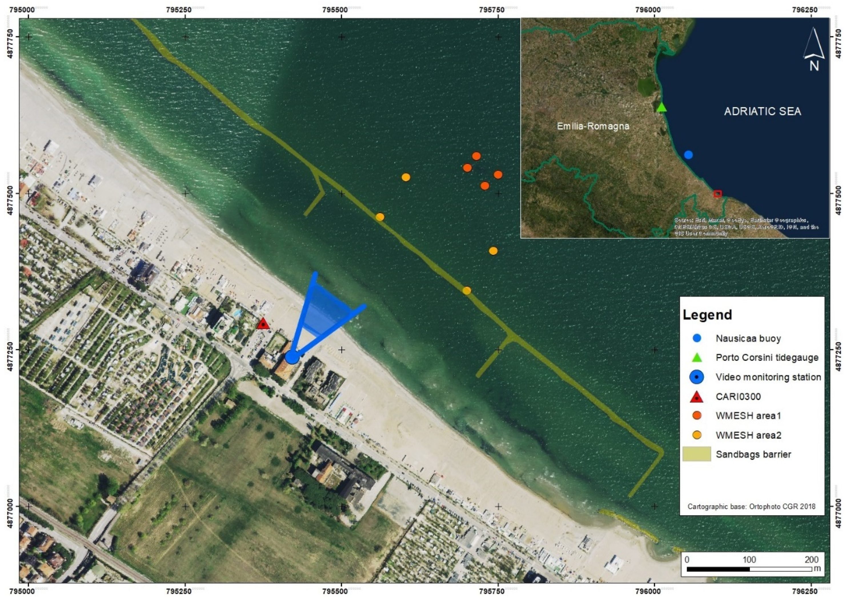
The study site is in the Riccione Municipality, a touristic locality in the southernmost part of the Emilia-Romagna Region (Italy) (Figure 1). This coastal stretch is about 400 m long; a 40–100 m wide sandy beach is backed by beach resorts on the Northern part and a free beach in the southern part, which is the site of this study.

This sector of the regional coast is lacking natural sources of sediment that originally came from Conca river mouth and from the erosion of cliffed coasts in the Northernmost Marche region thanks to a strong longshore drift directed from South to North [32].

Periodic topo-bathymetric surveys carried out by Arpae on the region’s coast [32,33,34,35,36] show that over last two decades, the beach has been in a state of “unsteady equilibrium/relative stability” regarding coastal erosion, thanks to repeated nourishment interventions. The site was, in fact, invested in by major nourishment projects realized at the regional scale in 2002, 2007 and 2016, and by several smaller-scale interventions carried out by the Riccione Municipality. In the submerged beach, a sandbags barrier was established in the 1980s at about 2 m depth (Figure 1) and is periodically reinforced. In 2018 and in 2020, the area was the site of experimental structures, i.e., prototype artificial concrete modules known as W-Mesh, to create an artificial habitat for organisms such as sibellaria and oysters. The W-Mesh modules were placed at a depth of about −4 m and −2.5 m and consist of a permeable, concrete structure (Figure 1).

Moreover, sediment displacement is periodically carried out on the beach-by-beach resort license holders by means of trucks in order to prepare the beach for winter storms. In the late Autumn, sand is usually replaced from the intertidal zone to the backshore to build an artificial embankment as a defence against the flooding of sea storms; in the spring season, the remaining sediment is relocated along the beach.

The meteo-marine climate in Riccione is characterized by sea storms mainly generated by northeasterly winds, named Bora, and southeasterly winds, named Scirocco, with the provenance of the latter frequently inducing the highest surge levels due to the larger associated fetch [16]. The littorals are subjected to low tidal variations, which span from a spring tidal range of ±0.4 m to extreme yearly values around +0.85 m. Sea weather conditions have a semi-permanent wave period of ≈4 s and a significant wave height of ≈0.5 m. High-intensity storm events can have wave height of up to 3.5 m each year and may reach 6 m every 100 years. Wave and climate data are available, respectively, from the Nausicaa buoy and the meteorological station at Cesenatico [33,34,35,36].

3. Materials and Methods

In the frame of the STIMARE project (STrategie Innovative, Monitoraggio ed Analisi del Rischio Erosione, www.progettostimare.it, accessed on 12 January 2022) [37], several surveys were performed between 2019 and 2021 to employ and compare different monitoring techniques. One of the goals of the project was to evaluate the morphological response of the studied beach to annual and seasonal wave regimes and to different coastal defense strategies [38].

All surveys were based on the same geodetic references. The planimetric reference system (RS) used was the ETRF2000-UTM32 (2008.0) EPSG: 7791. The CARI0300 topographic benchmark of the Emilia-Romagna Coastal Geodetic Network [33] was adopted as an altimetric reference for each survey to obtain not only the height correction (m a.s.l.) but also both the ellipsoidal/orthometric correction and to avoid possible bias due to different kinds of technical problems during field surveying.

Surveys were carried out every 6 months on the emerged and submerged beach during the project duration (see [38] for details); the date and techniques of the different surveys are reported in

Table 1. List of surveys and specific techniques employed: The low-cost VISTAE (Video monitoring Intelligent Station for Environmental applications); TLS (Terrestrial Laser Scanner); GNSS (Global Navigation Satellite System).

#	Date	Survey Technique
1	24 May 2019	VISTAE + TLS/GNSS
2	6 December 2019	VISTAE + GNSS
3	24 June 2020	VISTAE + GNSS
4	1 December 2020	VISTAE + GNSS
5	23 February 2021	VISTAE + TLS/GNSS
6	8 April 2021	VISTAE + TLS/GNSS
7	24 May 2019- ongoing	VISTAE

. In the present work, only data from the emerged and intertidal beaches are shown.

3.1. Video Monitoring

In the framework of the STIMARE project, a low-cost camera (VISTAE) was deployed on the southern Riccione beach for coastal video monitoring. It has been functioning since 24 May 2019 and it is still ongoing.

The Video monitoring Intelligent STAtion for Environmental applications (VISTAE) is a video monitoring system developed for coastal applications. It consists of a Raspberry Pi which controls a camera with a resolution of 2 pixels.

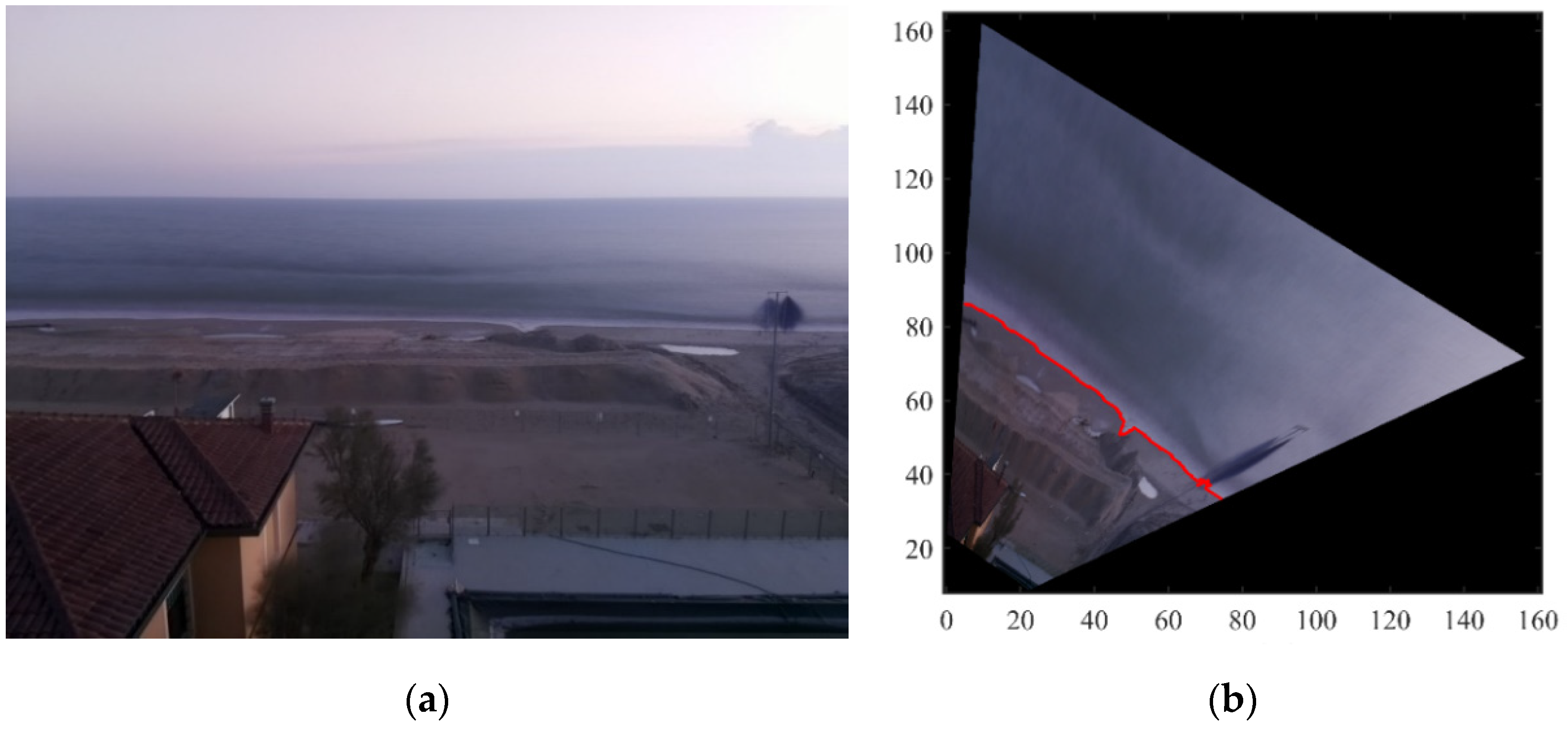
The VISTAE was programmed to acquire 1200 frames taken with a data rate of 2 Hz at the beginning of each hour during daylight (6–18 UTC). At the end of the acquisition, a single image (called time exposure image, timex) was extracted by averaging all the acquired frames and was sent to a remote server. Each day of acquisition, 13 timex images were collected and transferred for post-processing. First, a georectification procedure was applied, making use of a camera calibration and field calibration. The camera calibration, performed in the laboratory, minimized the lens distortion, while the field calibration transformed the image coordinates (in pixels) to ground coordinates (in meters). Both the field and camera calibrations were fundamental to correctly quantify the measured variables, such as the shoreline position, on the near-real time timex collected by the VISTAE.

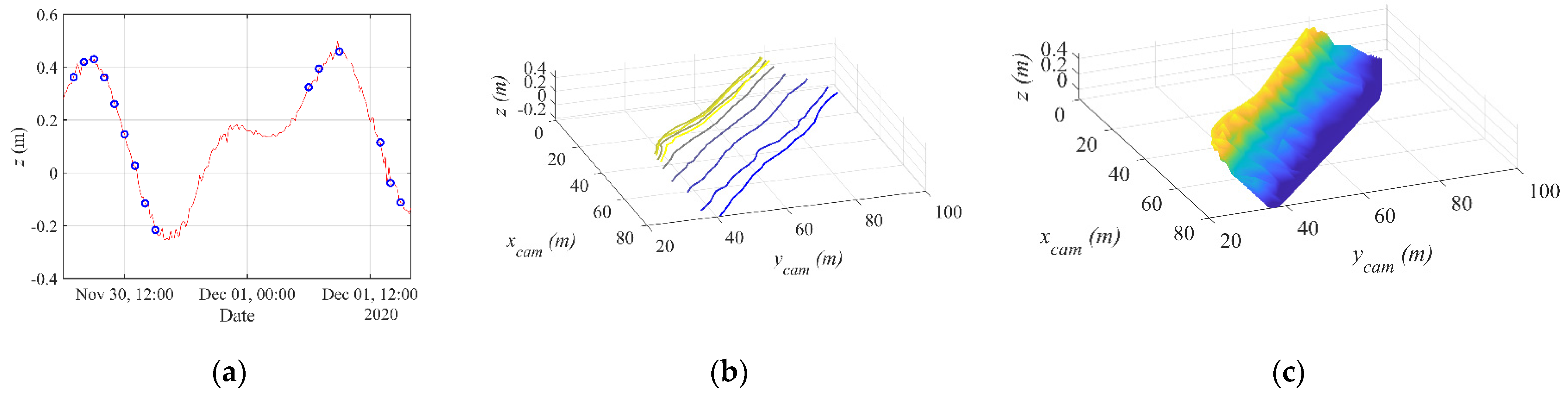
After georectification, a semi-automatic procedure was implemented in the analysis process. First, a shoreline detection algorithm extracted the shoreline from the timex. The automated shoreline detection was obtained on the original timex by an image segmentation technique [39]. Then, each shoreline was associated with the tidal level measured at the same time of the video acquisition.

For the identification of calm sea conditions, we defined a threshold of significant wave height H_s = 0.5 m, under which the wave setup could be ignored (see the discussion on the wave setup in the next paragraph). This last step allowed for the identification of the tidal measurements useful for the intertidal reconstruction. The matching between tidal measurements and shoreline detected at the same time yielded the reconstruction of the intertidal bathymetry during calm sea conditions (see Figure 2). The intertidal bathymetry was also defined as the swash zone, i.e., where the runup and runoff of the wave take place during a complete tide cycle. All the technical details of the new technology and of the extrapolation of the intertidal bathymetry (camera and field calibration, georectification, shoreline detection) are reported in Appendix A.

We remark that, as a first approximation, we did not include the wave setup in the analyses since, by adopting the aforementioned wave height threshold, H_s and T_m were small enough during the video acquisition. In fact, should we consider that, for our case, β ≈ 0.05 (beach slope), H_s ≈ 0.35 m (significant height) and L ≈ 14 m (wave length) The latter stems from the linear dispersion relation considering T_m ≈ 3 s and from the empirical relation by [40,41] in which the wave setup results in <η> = 0.35 β (H_s L)^0.5 < 0.04 cm, which is within the expected uncertainty (see Section 5). We then compared the detected shoreline position and intertidal bathymetry with the results of the in-situ measurements described in Section 3.2 (TLS and GNSS). The extension of the area covered by video camera measurements varied between 620 m² and 1975 m² and could be extremely variable. This depended on the tidal excursion which occurred in a restricted time range (2–5 days) immediately before and/or after the field survey. In this work, one of the aims was to compare the VISTAE’s data with diurnal field surveys. For that reason, it was decided to use the camera only during daylight hours. However, it should be highlighted that the Raspberry Pi could easily handle the implementation of a very low-cost INR sensor to take pictures and to detect shorelines also during nocturnal time. This is possible thanks to the flexibility of the system deployed and is available for future developments.

Finally, it is important to evaluate the expected resolution of the camera in order to get some idea of the uncertainty involved. The spatial resolution of the system can be evaluated as follows [8]:

Δc = Rδ/L_x,pix = (2R/L)atan(L_x,m/2f),

(1)

Δr = Δc R/z_c,

(2)

where R is the slant range distance from the camera, δ is the angular field of view, f is the focal length, L_x,pix and L_x,m are the number of pixels and sensor size, respectively, z_c is the height of the camera with respect to the measured surface, and Δc and Δr are the pixel resolutions in the cross and radial directions, respectively. By considering a distance range comparable with our observation (R = 100 m), we obtain a spatial resolution of Δc ≈ 0.05 m and Δr ≈ 0.5 m. The observed shoreline was ≈120 m long and the corresponding emerged beach was ≈50 m wide. Based on the report by [33], and by considering a tract from the emerged beach to the isobath equal to −2.5 m, the volume variation was about 23 m³/m during the period 2012–2018. With these data, we could expect a height beach variation of the order of 0.1 to 1 m.

3.2. Field Surveys

Surveys 1, 5 and 6 (Table 1) were carried out using TLS and GNSS techniques. TLS provided high-resolution topographic data suitable to produce Digital Terrain Models (DTMs) at the centimetric resolution, which are commonly used in quantitative land-surface analysis [42] and in other geosciences applications. The distance measurements were extremely precise and accurate thanks to “Phase-shift” technology, a measuring method based on the phase difference between the emitted laser light and the returning radiation after its reflection on the investigated surface.

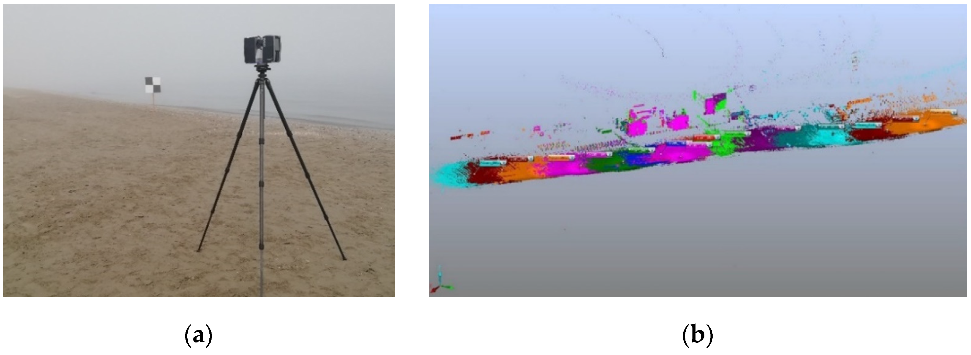
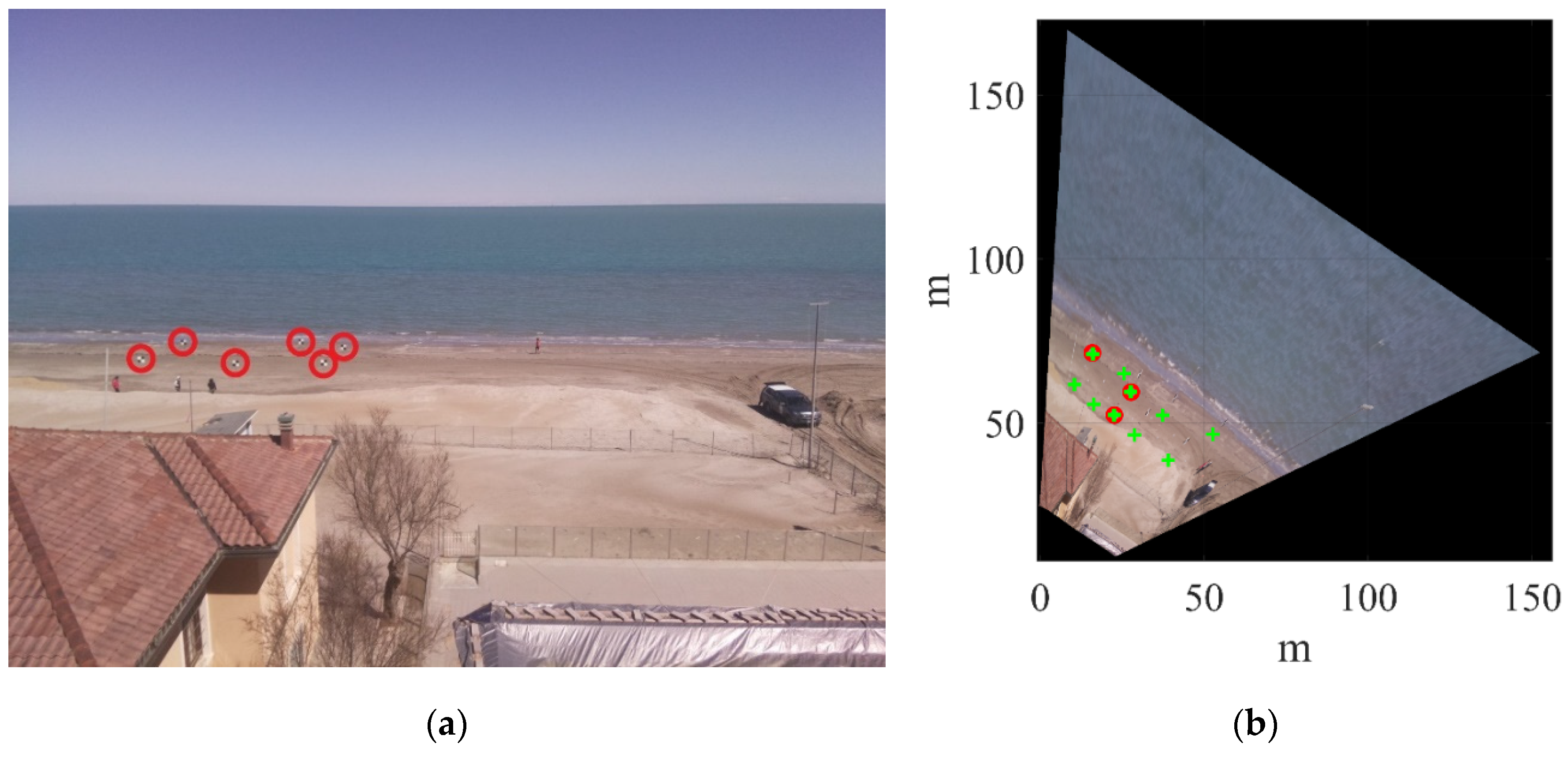
For TLS measurements, a FARO Laser Scanner Focus^3D (Figure 3a), which emitted a laser light in the NIR range (905 nm), was used. The scans were set to 1/3 of the full resolution, producing 3D point clouds with a resolution of 6 mm at 20 m distance [43]. Fifteen scans were acquired at each position, with 50% of these overlapping each other (Figure 3b), and were georeferenced by means of chessboard targets distributed on the scan area (Figure 3a). The targets were 50 cm² chessboards in black/white colors (with very low and very high reflectance, respectively) mounted on a wooden pale 1.5 m-high: the target centers provided a materialized point easy to survey, both via GNSS (with the adequate antenna offset) and via TLS.

The principal post-processing phase involved FARO^® SCENE (FARO, Lake Mary, FL, USA), a dedicated software package that is essential for registration of scans, the operation that determinates the spatial relations of scans and the transformation from a “relative internal” RS to an “absolute coordinate” RS. In this case, the registration of scans was performed by automatically matching corresponding points between adjacent scans, directly identified by the operator or automatically by software (“target to target” methodology [44]).

After the scan registrations, the clouds were directly processed, deleting irrelevant objects (people, targets, building, etc.) by means of Cloud Compare software (an open-source software for 3D clouds analysis, Telecom ParisTech and EDF R&D, Paris, France) and the SOR filter (Statistical Outlier Removal). In order to fill small gaps, the whole cloud was meshed (surface creation via Delaunay triangulation) and resampled (5 mm-spaced points) to obtain the definitive unique point cloud, exported as a generic ASCII text file. Finally, the Global Mapper software (Blue Marble Geographics, Hallowell, ME, USA) was used to convert it into an Arc ASCII Grid, another ASCII format suitable for working with GIS software, gridded to 0.10 × 0.10 m. The same operations were applied to all TLS surveys (Table 1). In survey 2 of the emerged beach, and in specific field calibrations of VISTAE-acquired data (surveys 3 and 4), a GNSS-NRTK topographic survey was carried out. Indeed, despite TLS being the most accurate instrument and allowing for a complete surveyed surface without data interpolations, it is a time-expensive technique and needs three operators to work it. A GNSS-NRTK survey, on the contrary, allowed for a more rapid survey (depending on the distance between consecutive transects) and needed only one operator, but its best precision (±5 cm at most) was obtained only on the directly surveyed points, with data interpolation operations being performed for the remaining area, resulting in a lower level of precision. The surveys were carried out measuring coordinates at consecutive points approximately every 2 m along transects with different orientation (long-shore and cross-shore). After the appropriate point transformations and corrections, a TIN (Triangulated Irregular Network) surface was generated with GIS software. TIN is a continuous surface formed by triangular facets where the triangle’s vertices are the points surveyed with the elevation information. The TIN surface was then converted into a raster grid (Arc ASCII Grid), 0.10 × 0.10 m gridded. The same operations were applied to all the GNSS-NRTK surveys (Table 1). The 3D surface models generated through the operations described above were then compared via ESRI ArcMap 10.5 software (Esri, Redlands, CA, USA).

3.3. Comparison between Field and Remote Measurements

The data acquired on the emerged beach in surveys 2, 4, 5 and 6 through different techniques were compared (see Table 1), while the data from surveys 1 and 3 were not used for comparison in this paper due to technical problems relating to the VISTAE, e.g., its limited visibility resulted in a very-low image quality. The intertidal beach was extrapolated from the VISTAE (Section 3.1), and the vertical coordinate was compared with the 3D model extracted from GNSS and TLS (Section 3.2) for the overlapping observed area. For GNSS surveys, three cross-shore transects corresponding to the field measurements were also extracted from the VISTAE observations and then compared. For comparison on the coastlines at the time of different surveys, the zero contours were extracted by each DTM, since the topographic zero (0 m a.s.l.) was selected as a proxy of the coastline position [45].

The planimetric distance between the two reconstructed zero contours (through the VISTAE and GNSS surveys) was calculated using DSAS v5.0 software [46], an open-source software realized by USGS (United States Geological Survey) for shoreline analysis that works in ESRI ArcMap as an add-in. Usually, DSAS is utilized for shoreline displacement analyses over time, but in this case, we applied it to compare two simultaneous shorelines extrapolated by two different monitoring techniques, i.e., field measurements and remote observations. DSAS automatically generated perpendicular transects, starting from a baseline (selected by the operator), spaced every 5 m in this case. Through DSAS, several statistics were obtained in relation to the intersection points between each transect and the reconstructed shorelines: in this case, the NSM (Net Shoreline Movement) statistics, i.e., the distance between the two shorelines, could be computed.

As an additional method, a MATLAB script was developed and adopted to calculate the horizontal distances and hence the NSM. In this case, the horizontal distance between the two shorelines was calculated using the GNSS measurements as a reference in the horizontal projection. The method was as follows: a perpendicular line started from the midpoint of each segment, joining two adjacent nodes of the GNSS-extracted shoreline; the intersection between the perpendicular line and the camera shoreline determined the single distance, Δd_i. The mean distance, Δd, was defined as the mean of the N single distances, Δd = Σ Δd_i/N (see Figure 4). This resulted in a different mean horizontal distance, Δd, with respect to DSAS, depending on the number of transects selected to extract the NSM.

4. Results

We compared the reconstructed intertidal beach and the extrapolated shoreline from field and remote measurements of the observed beach stretch, and the transects measured by GNSS-NRTK and VISTAE.

The mean difference, the standard deviation and the RMSE are reported in

Table 2. Synthesis of the comparison between field measurements (GNSS-TLS) and remote data (VISTAE). 3D elevation model and transects refer to vertical distances, while the NSM (Net Shoreline Movement) obtained by means of DSAS indicates horizontal distances (MATLAB results are between parentheses). “Δz_m”, “st.d.” and “RMSE” stand for mean difference, standard deviation and root mean square error, respectively. “tr1”, “tr2” and “tr3” stand for transects 1, 2 and 3, respectively.

Survey		3D Model (m)			Transects (m)			NSM (m)
#	Method	Δzm	st.d.	RMSE	Δzm	st.d.	RMSE	Δd	st.d.	RMSE
2	GNSS	−0.02	0.03	0.04	tr.1: 0.08	0.01	0.08	1.06 (0.68)	0.74 (0.50)	0.87
					tr.2: 0.07	0.05	0.08
					tr.3: 0.01	0.03	0.02
4	GNSS	−0.05	0.07	0.09	tr.1: 0.03	0.04	0.04	−1.99 (−0.92)	2.37 (2.08)	2.27
					tr.2: 0.04	0.04	0.07
					tr.3: −0.04	0.05	0.03
5	TLS	0.00	0.07	0.07	n/a			n/a
6	TLS	−0.02	0.05	0.05	tr.1: −0.01	0.02	0.01	−1.38 (−1.34)	0.47 (0.44)	1.41
					tr.2: 0.02	0.05	0.06
					tr.3: 0.03	0.02	0.05

for four selected surveys. These values were obtained by comparing (i) the vertical measurements of 3D elevation models and three cross-shore transects and (ii) the horizontal NSM (Net Shoreline Movement). We have separately introduced the results for the cases in which field measurements are represented by GNSS-NRTK (selected surveys 2 and 4) and by TLS (surveys 5 and 6), respectively. The details of the analyses and the results are illustrated in Section 4.1 and Section 4.2.

4.1. Comparison between VISTAE and GNSS Surveys

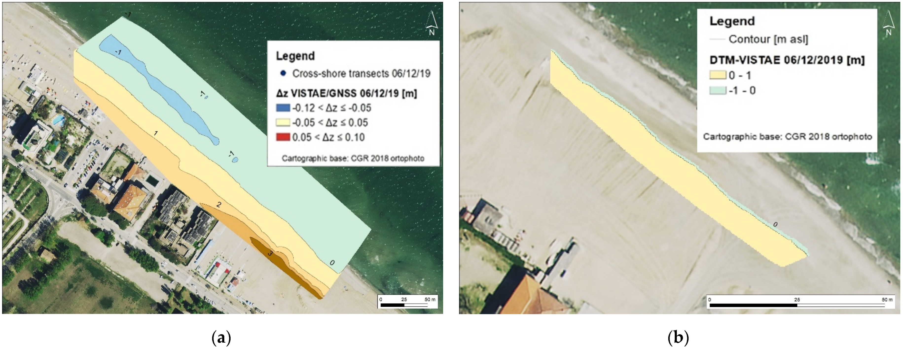
Surveys 2 and 4 allowed for a comparison between the GNSS and VISTAE surveys (see Table 1). Figure 5 shows an example of the 3D surface reconstructions from the GNSS survey and the VISTAE (panels a and b, respectively). DTMs generated by direct field surveys (GNSS) included an area about 400 m wide, from the intertidal zone to the inner backshore. DTMs generated by the remote VISTAE data covered a smaller area, about 100 m wide and 20 m long, corresponding to the intertidal zone of the beach sector included in the camera shooting area (see Figure 1). In this case, the tidal level used for the reconstruction of the intertidal bathymetry and the significant wave height H_s referred to 5–6 December 2019. The background photo on which the intertidal beach bathymetry is represented in Figure 5, Figure 6, 8, 10 and 11 is an orthorectified image taken from the Regional Service Portal (http://geo.regione.emilia-romagna.it/cartografia_sgss/user/viewer.jsp, accessed on 12 January 2022). As the intertidal beach bathymetry location depends on the tidal range of the acquisition time of the isobaths, it can be represented on the beach, as in Figure 5.

Figure 6a reports the elevation difference, Δz, represented in three classes: negative differences are in blue, a central class with a range of ±0.05 m, which indicates no significant elevation difference (range of GNSS precision), are in light yellow and positive differences are in red. This comparison for survey 2 provided a strong correspondence between the two models, with a mean value and standard deviation equal to (−0.02 ± 0.03) m and with 77% of data in the central class (see histograms in Figure 6c and Table 2).

Also, cross-shore transects (Figure 6a and Figure 7) were used for comparing the two methodologies on punctual, single measures, thus with more precision than the DTM-interpolated area. For transects 1 and 2, the elevation differences were Δz₁ = (0.080 ± 0.001) m and Δz₂ = (0.068 ± 0.054) m, respectively, while the result of transect 3 showed a very good overlap with Δz₃ = (0.007 ± 0.026) m (Table 2). The comparison of the VISTAE and GNSS elevations show a very good fit between measures, with an R² = 0.92 and an RMSE = 0.036 m (Figure 6d).

Figure 6b shows the NSM (Net Shoreline Movement) calculated from the GNSS and VISTAE data acquired during survey 2. There was a good overlap (≤0.5 m) in the shoreline position in the North-Western (NW) part of the observed area, while in the central and South-Eastern (SE) areas, the VISTAE systematically overestimated the NSM position with respect to the one extracted from field measurements. For this case, the NSM range was between −0.53 m and 2.36 m; the mean value and standard deviation were (1.06 ± 0.74) m using DSAS method, while, using MATLAB, the mean value Δd and standard deviation had the same sign but were smaller, i.e., (0.68 ± 0.50) m. The different results were due to the different techniques used, as DSAS used transects drawn each 5 m while the MATLAB script used one transect each ≈ 0.2 m. 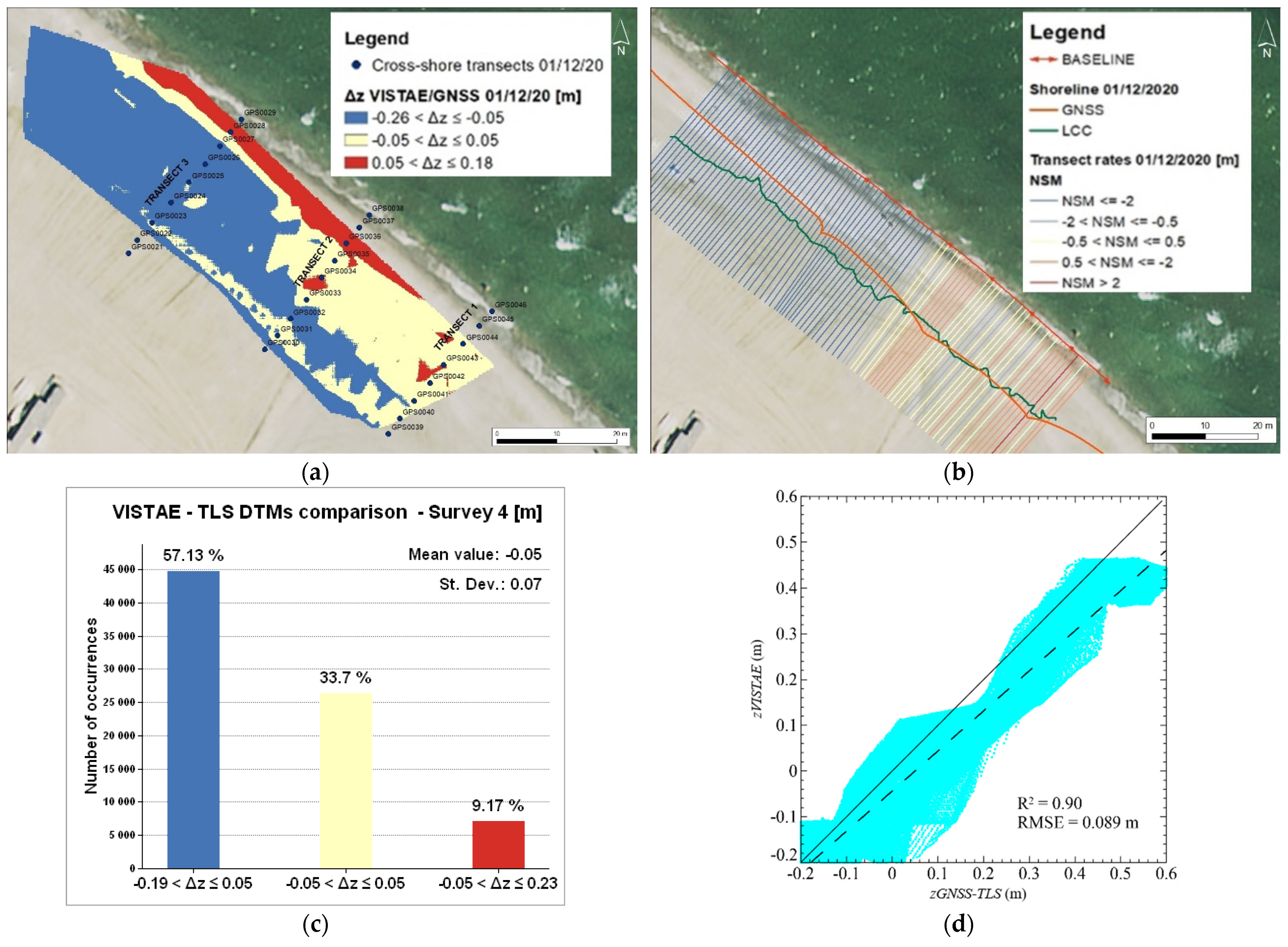Consequently, higher discrepancies became relatively more significant for the DSAS method and augmented the overall Δd.

Similar analyses were made on the field and remote data of survey 4. In this case, images from 30 November–1 December 2020 were used to reconstruct the VISTAE intertidal bathymetry. The height comparison (Figure 8a) showed an overall strong correspondence between the two models, with a mean value and standard deviation of Δz = (−0.05 ± 0.07) m, but in this case, the VISTAE data showed a general underestimation, with 57% of the data as negative differences (Figure 8c). It could be noted that Δz values within the central class were mostly observed in the south-eastern part of the beach, whereas negative differences prevailed in the central and north-western part of the surveyed area. Positive differences were mostly concentrated in a narrow belt close to the shoreline. This result could possibly be due to a limited extension of the ground control points (GCP) in the most north-westerly part of the surveyed area. However, these limits can be easily overcome in future applications. Furthermore, the comparison of the VISTAE and GNSS elevations show a good fit between measures, with an R² = 0.90 and an RMSE = 0.089 m (Figure 8d).

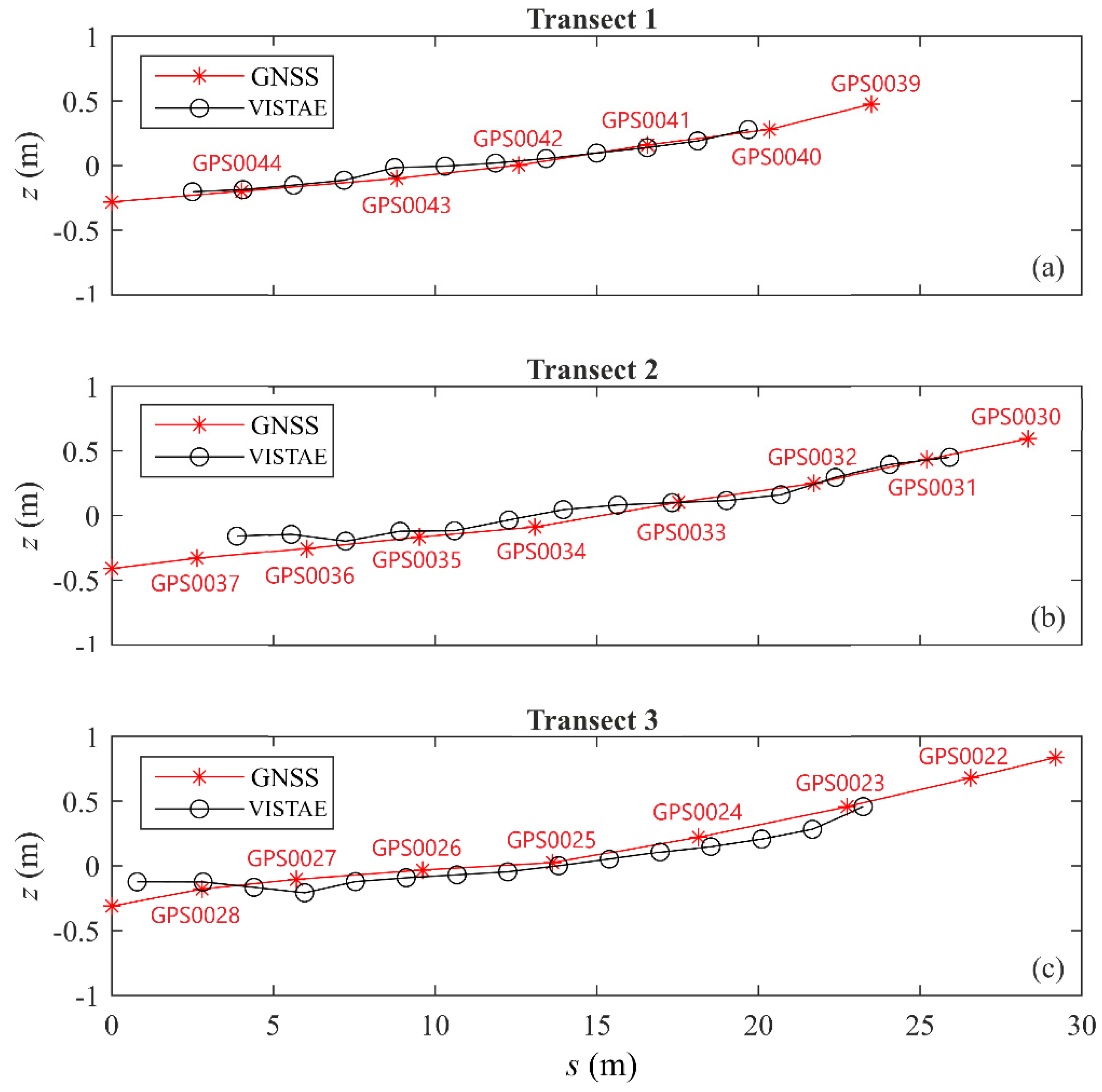
Figure 9 shows the comparison between field measurements (GNSS) and remote data (VISTAE) concerning the transects. The results confirmed what has already been observed from 3D elevation models: transects 1 and 2 were well aligned, with a slight overestimation of the VISTAE data, while in transect 3, the VISTAE data were systematically below the GNSS measurements (with an exception seaward). Numerically, the elevation differences for transects 1 and 2 were Δz1 = (0.028 ± 0.039) m and Δz2 = (0.041 ± 0.044) m, respectively, while for transect 3, the height difference was negative and resulted in Δz3 = (−0.038 ± 0.054) m (Table 2). The RMSE values yielded the same conclusions.

Figure 8b reports the shoreline NSM calculated from the GNSS and the VISTAE for survey 4 using DSAS. The NSM range was between −6.27 m and 2.28 m; the mean value Δd and standard deviation resulted in (−1.99 ± 2.37) m, while the RMSE was 2.27 m. Using MATLAB, the mean value Δd and standard deviation had the same sign but were smaller, i.e., (−0.92 ± 2.08) m (Table 2).

From both methods the results suggested that, in this case, it would be beneficial to reduce the observed domain of the camera to improve the overall accuracy by eliminating the edges, where higher errors emerged (in particular to the NW). In fact, by disregarding the edges of the VISTAE field of view, the NSM mean value and standard deviation could be reduced up to (−0.31 ± 1.35) m.

4.2. Comparison between VISTAE and TLS Surveys

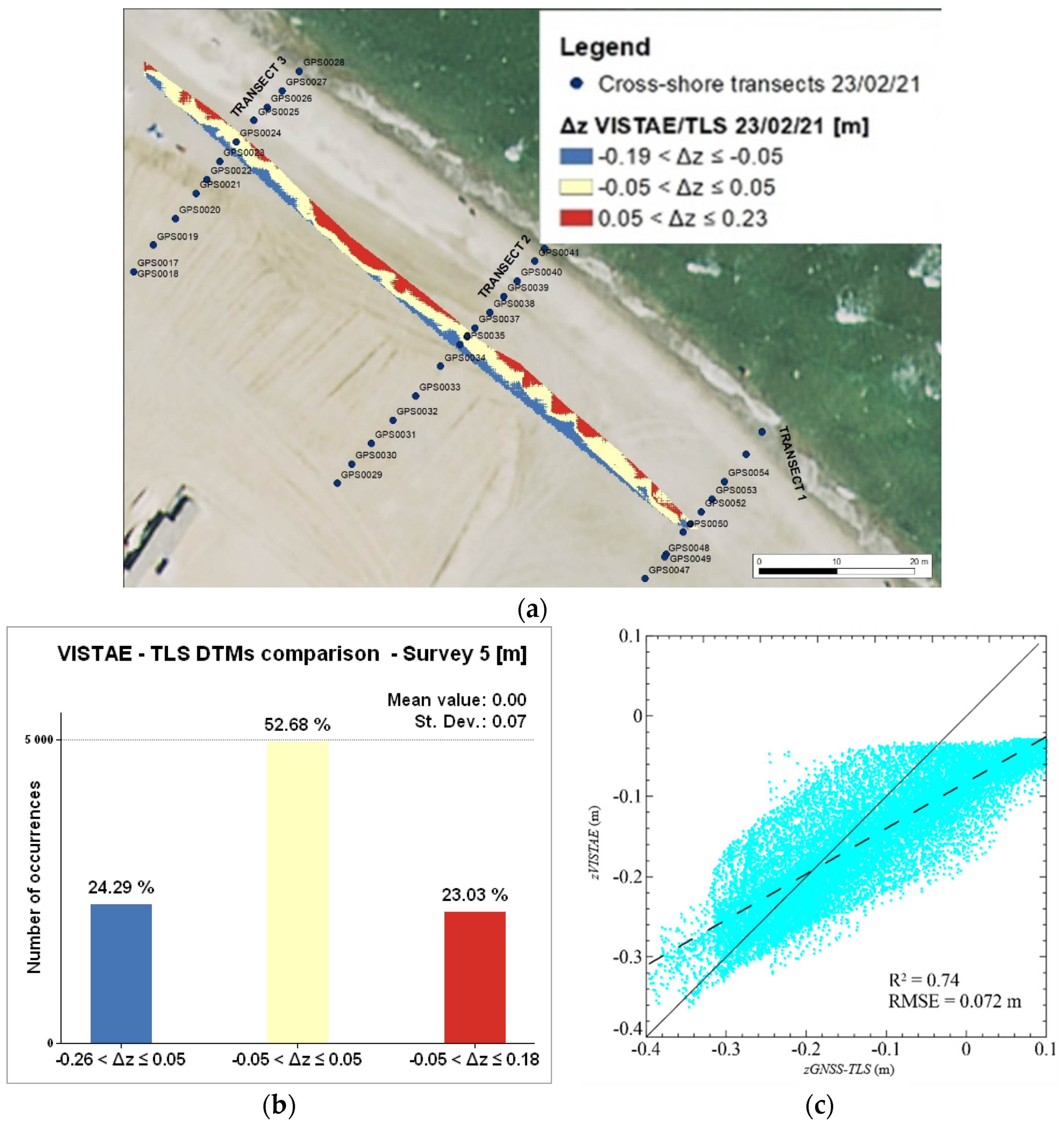
Data collected in surveys 5 and 6 (Table 1) are here reported.

For survey 5, the images used to extrapolate the intertidal bathymetry from remote measurements were taken on 21–23 February 2021. The elevation difference, Δz, represented in the three classes in Figure 10a, showed a very strong correspondence between the two models, with a mean value and standard deviation of (0.00 ± 0.07) m, 52% of data in the central class and a smaller percentage of higher differences, both positive and negative, mostly observed seaward and landward, respectively (Figure 10b). The comparison of the VISTAE and GNSS elevations show a less good fit between measures, with an R² = 0.74 and an RMSE = 0.072 m (Figure 10c), suggesting that taking into consideration only the mean difference in this case could be misleading.

For survey 5, the comparison of the coastline position and of the transects was not carried out because the tidal level was too low during the weeks before and after survey 5, and the tidal excursion was limited, so that the coverage of the VISTAE data did not include many transects points of field measurements. We remind that the VISTAE data represented the intertidal bathymetry during the observed period, and this limited the use of the NSM analysis in some cases.

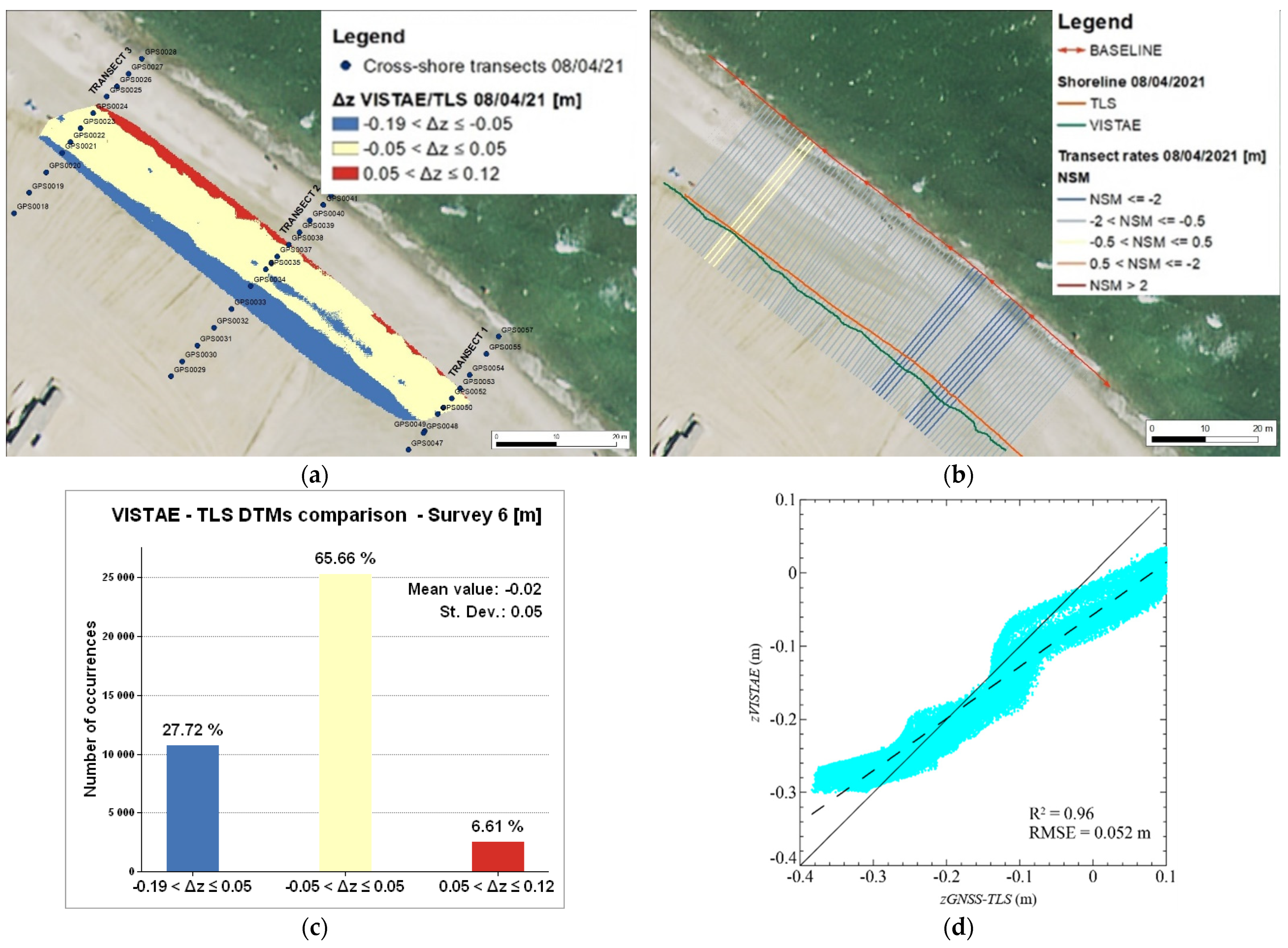
For survey 6 (8 April 2021), tidal data used to reconstruct the VISTAE intertidal bathymetry were obtained on 7 April 2021. The height areal comparison (Figure 11a) showed a strong correspondence between the two models, with a mean value and standard deviation of (−0.02 ± 0.05) m for the elevation difference, Δz, 65% of data being in the central class and smaller percentage of higher differences, both positive and negative, again mostly located seaward and landward, respectively (Figure 11c). The comparison of VISTAE and GNSS elevations show a fairly good fit between measures, with an R² = 0.96 and an RMSE = 0.052 m (Figure 11d).

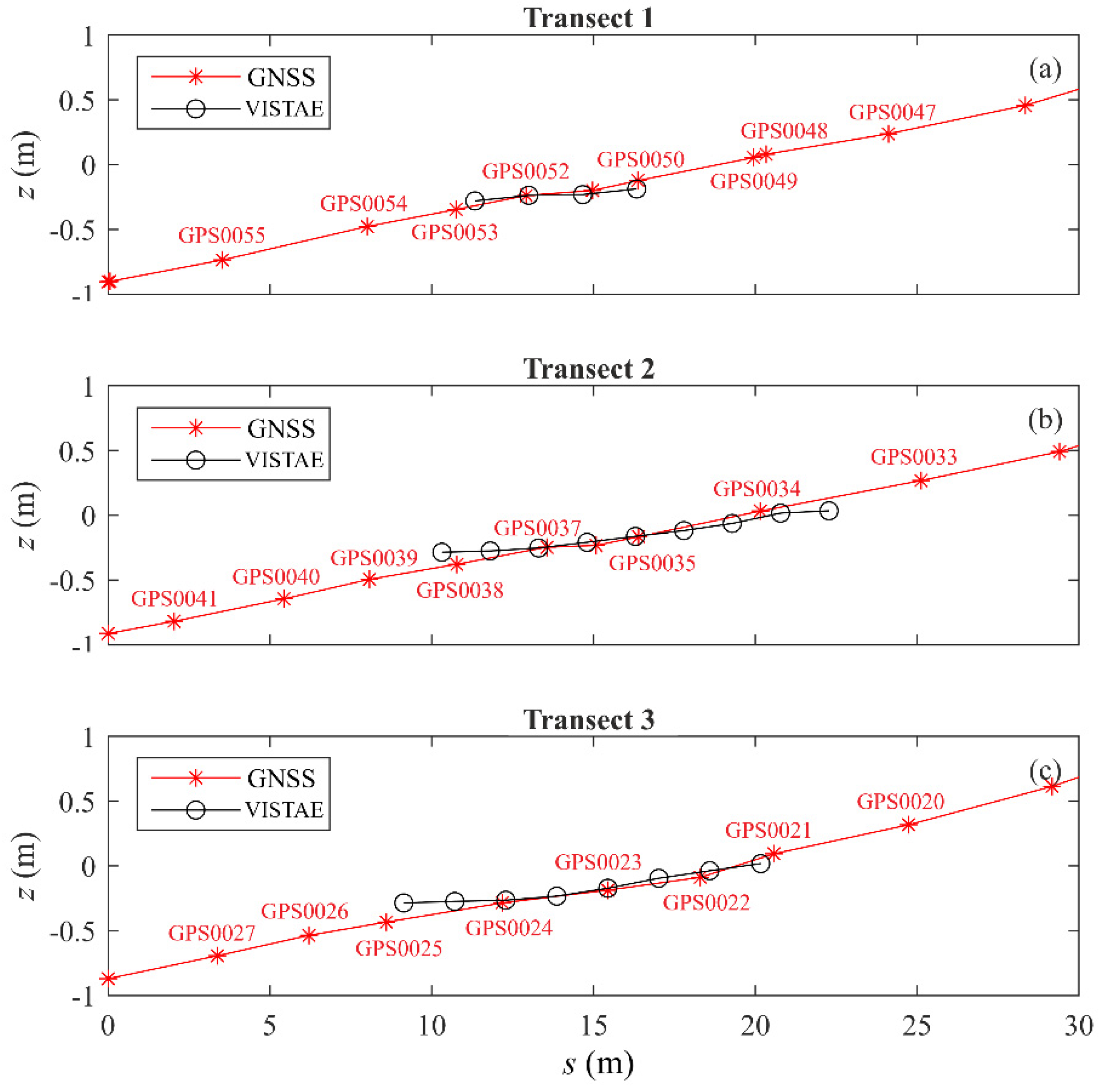
Figure 12 reports the comparison between field measurements (TLS) and remote data (VISTAE) concerning the transects. The results showed a significant overlap for all the three transects investigated, with elevation differences equal to Δz₁ = (−0.013 ± 0.019) m for transect 1, Δz₂ = (0.017 ± 0.053) m and Δz₃ = (0.026 ± 0.015) m for transects 2 and 3, respectively.

Figure 11b shows the NSM calculated for the zero contours comparison between TLS and VISTAE data for survey 6 (8 April 2021). The NSM range was between −2.39 and −0.45 m; using the DSAS method, the mean difference Δd and standard deviation were (−1.38 ± 0.47) m, while for MATLAB they were (−1.34 ± 0.44) m.

5. Discussion

The strengths and limitations of different technologies adopted for beach surveying should be evaluated to better exploit their complementarity and integration [47]. In our case study, image-derived surveys were particularly effective at capturing beach variability in continuum or very frequently during the daylight, without the efforts and costs associated with field survey techniques that, on the other side, provided a high-accuracy three-dimensional reconstruction of the beach morphology.

The comparability between field (GNSS, TLS) and remote, video-derived (VISTAE) measurements is reported in Table 2 by using the 3D models and three transects for the elevation. The mean elevation bias was in the range −0.08 m < Δz < −0.04 m, while the standard deviation was in the range 0.01 m < st.d. < 0.07 m and the RMSE was between 0.01 m and 0.09 m. In our analysis, RMSE and mean bias were proxies of the expected accuracy, while the standard deviation indicated the precision and, as a further source of information, the nature of the uncertainty (i.e., if it stemmed from systematic or random errors). If the field measurements by GNSS-TLS were intended as a validation of the camera data, Δz, standard deviation and RMSE could be considered as a proxy of the camera performance in the vertical direction. On the other hand, the expected uncertainty in the horizontal direction, derived from the mean distance Δd, the standard deviation and the RMSE of the net shoreline movement (NSM), was of the order O(1 m), calculated on horizontal planes without considering the elevation since this was a low-gradient beach.

To evaluate the potential and applicability of the instrumental approach presented in this paper with respect to camera performances adopted elsewhere,

Table 3. Comparison of the performance of the VISTAE with recent literature dealing with coastal monitoring through field surveys and remote sensing data, in terms of vertical (Elevation) and horizontal distances.

Paper	Method	Elevation			Horizontal
		Mean distance (m)	Standard deviation (m)	RMSE (m)	RMSE (m)
Plant et al. (2007) [17]	Nearshore camera	−0.38–0.04	n/a	0.10–0.40	n/a
Harley et al. (2011) [47]	Nearshore camera	n/a	0.15	0.15	1
Didier et al. (2017) [48]	Nearshore camera	−0.04–0	0.06	0.06	0.27–0.52
Andriolo et al. (2018) [49]	Nearshore camera	0.04–0.06	0.04–0.07	n/a	0.52–0.64
Laporte-Fauret et al. (2019) [50]	UAV	−0.10–−0.02	n/a	0.05–0.13	n/a
VISTAE	Nearshore camera	−0.04–0.08	0.01–0.07	0.01–0.09	0.87–2.27

shows a comparison between the VISTAE and similar technologies presented in the literature. The video camera data obtained in the present paper showed an accuracy comparable with these, or even higher, if compared with recent applications (see, e.g., [16,17,47,48,49,50]). Similar values could be found also in [20], where the vertical RMSE was up to 0.34 using a fully automatic shoreline detection model, and in [22], with an RMSE equal to 0.26 m. However, unlike previous video camera systems, the VISTAE also maintains the advantages of low costs, the availability of continuous surveys during daylight and the novelty of programmability (which yielded autonomous data acquisition and analysis).

As a means of double checking the accuracy, the estimation of the NSM was based on the use of the ad-hoc made scripts with MATLAB and a commercial code (DSAS). In the results presented here, the former analysis provided better performances for all the indicators (mean, RMSE and standard deviation).

A careful observation of the errors (and their distribution) can yield some insight into the overall accuracy. Consider Survey 6 as an example. A close inspection of the intertidal beach data revealed that positive differences (higher values of the VISTAE data) were concentrated seaward, while negative differences were gathered landward. The errors were concentrated near the boundaries of the field of view, where the GCP were sparse. Our data also suggest that not considering the edges of the camera field of view (where distortion effects are higher, especially if laboratory and field calibration are not well conducted) can reduce uncertainty to one third of its initial value. For the same survey, the shoreline comparison indicated that the error was mostly systematic (low standard deviation) and caused an underestimation of the shoreline position. We remind also that Δd was calculated on a horizontal plane (i.e., by using only horizontal ground coordinates) and it was expected that it might report remarkably higher values than the elevation difference for low-steepness beaches. Potential sources of discrepancy with in-situ measurements can be the difference between the local tidal level and the measured one, a tidal modulation of the swash zone processes, errors in photogrammetry, wind-induced setup and discontinuous or complex intertidal bathymetry [18].

Further studies are necessary to establish the real potential of the VISTAE. We have carried out a study on a low-steepness beach, but there is no reason to believe that high-gradient beaches could not be adequate to conduct similar analyses (shoreline, intertidal bathymetry, etc.). In that case, installing the system at a significantly high location would be strongly suggested to adequately observe steeper morphologies and to reduce the distortion effects of the rectification process.

One idea which might improve the performance of the camera would be to change the orientation of the camera with respect to the shoreline, which was not possible in our case due to the limitations of the installation site. We oriented the camera in the cross-shore direction, obtaining a field of view of ≈120 m, but pointing the camera in the long-shore direction would allow for the investigation of a wider field of view. In that case, it would be possible to compare the accuracy of the camera in the near- and far-fields and to check what area extension could be investigated within a fixed uncertainty. We refer to previous studies cited above and consider the distance of the camera from the shoreline and the spatial variation of the errors. The spatial resolution obtained from [8], in our distance range, was Δc ≈ 0.05 m and Δr ≈ 0.5 m. Referring to Table 3, [47] reported a slant range distance R ≈ 1300 m long-shore (with z_c = 44 m), [48] reported R ≈ 300 m (with z_c = 12 m), while in [49], R ≈ 60 m. From these results, it is evident that changing the camera orientation in the longshore direction and moving the camera to a higher position would significantly improve the resolution. As the spatial resolution of the camera is strictly related to the errors, we would expect those improvements to allow a slant range distance several times larger than the current one without affecting the overall uncertainty.

Another possible application could be the use of multiple cameras with overlapping zones to augment the extension of the observed coast. Regarding the deployment of the VISTAE in remote areas without power, an ongoing study carried out in the framework of a project funded by the Emilia-Romagna Region, Italy (TAO project, www.tao.consorzioproambiente.it, accessed on 12 January 2022) is testing the use of a solar panel coupled with a car-type battery. The whole system, although not simple to install due to the larger size, would gain the great advantage of being completely independent of an electric power supply. In the framework of the same project, another camera has been installed in a different coastal area, with the implementation of an open-source library through Python at all the levels for fully automated data acquisition and analysis. The collection of the results is still ongoing and not yet available.

6. Conclusions

In this paper, we performed integrated field and remote measurements using a GNSS, TLS and VISTAE, in a coastal tract in Riccione (Northern Adriatic Sea, Italy). Then, we analyzed and compared the results in terms of accuracy between the different technologies used.

The video monitoring system applied in our work was realized with a low-cost programmable technology (Raspberry Pi) which, to the best of our knowledge, has never been applied in coastal engineering, while its use is currently expanding in other fields (see Section 1). Its greatest advantages are its very-low cost and the possibility to automatize and program the long-term monitoring and analyses of the observed beach, through which we were able to retrieve important parameters for evaluating the morphological evolution of the beach (e.g., the shoreline, intertidal bathymetry and many others). Here, it has been shown that this new technology can be applied for coastal monitoring studies with the extrapolation of quantitative data, if accurately calibrated through GCPs. For quantitative studies, in fact, the use of a VISTAE as a complemented system with well-known field survey techniques, such as GNSS and TLS, has been demonstrated to produce reliable results by carefully analyzing the main statistics (RMSE, main difference, standard deviation) both for the elevation (vertical) and horizontal distances when compared to similar approaches in the literature. Furthermore, our results suggest that careful laboratory and field calibrations are compulsory to reduce uncertainty and obtain an adequate accuracy, with these also relying on the correct coupling of the VISTAE data to the high-spatial resolution data obtained from field measurements. However, we recognize that the accuracy of the video monitoring technique can sometimes be site-specific. The system can be improved in several different ways (fully automated analyses, open-source software, autonomous power supply, etc.) thanks to its easy programmability.

In synthesis, the overall comparison shows that the VISTAE is suitable for coastal video monitoring and can provide quantitative, reliable results if adequately coupled with field measurements. We found that accuracies obtained using the VISTAE are comparable to those obtained using other techniques in the literature, and that the VISTAE present novel features such as a low-cost and flexibility. We believe that this combined approach can provide long-term data with both high temporal and spatial resolutions at very low-cost, with high flexibility in terms of deployment and remote control, and with easy automatization of data acquisitions and analyses. The presented technologies will, in the future, provide a useful tool for the assessment of flooding hazards and vulnerability.