
Modeling Reference Crop Evapotranspiration Using Support Vector Machine (SVM) and Extreme Learning Machine (ELM) in Region IV-A, Philippines


Abstract
:1. Introduction
2. Materials and Methods
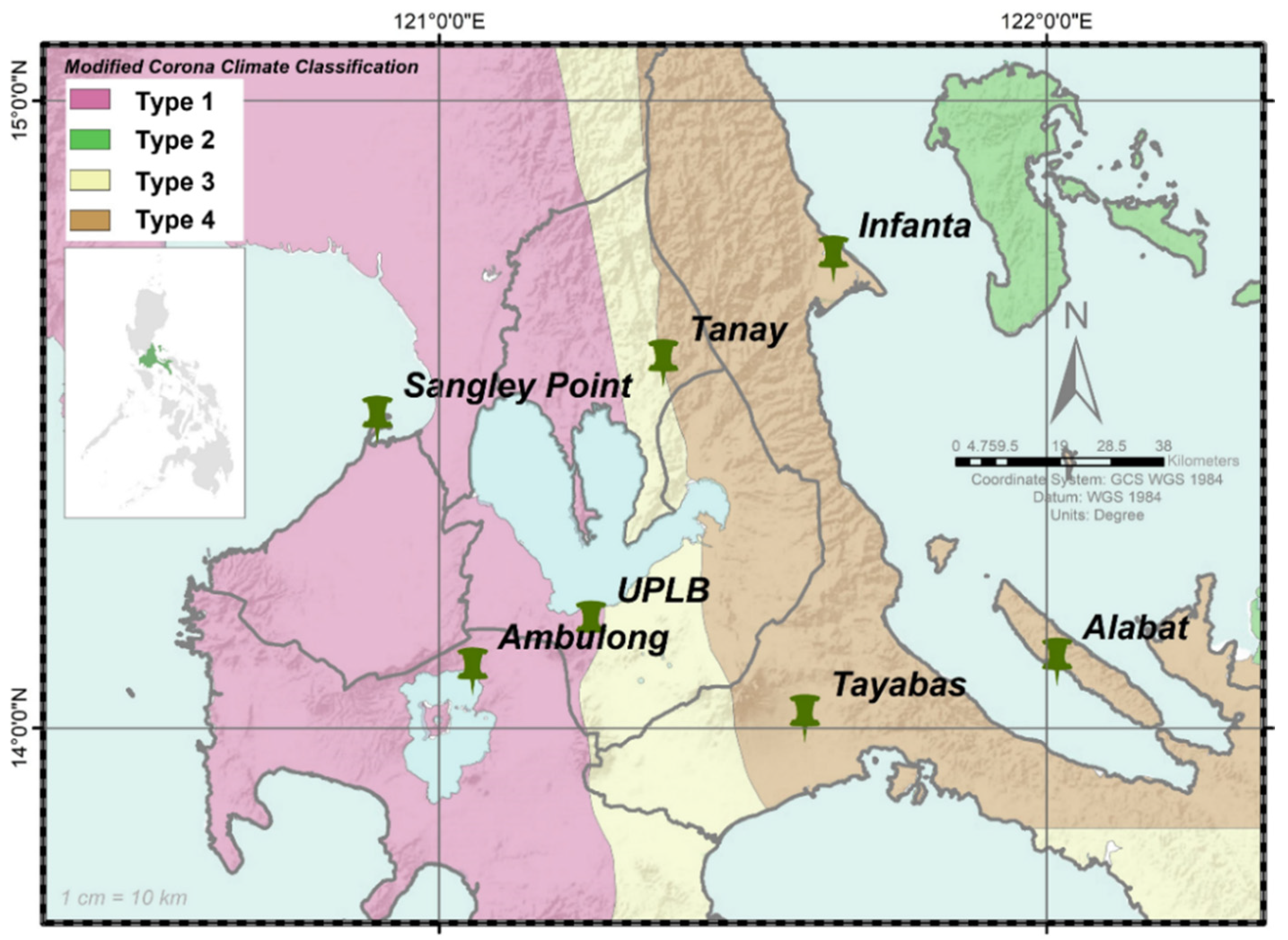
2.1. Study Area
2.2. Empirical Models for ETo Estimation
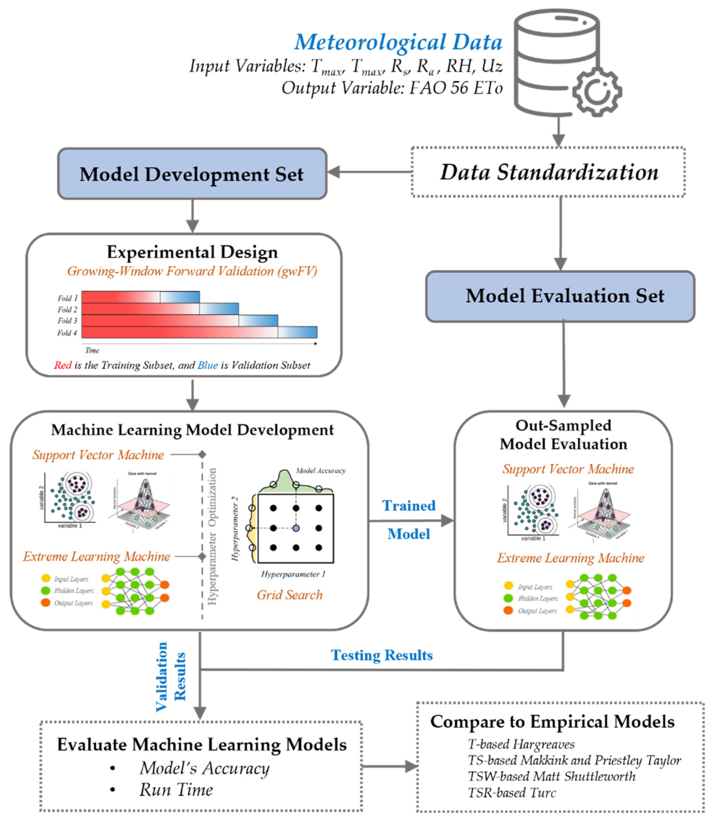
2.3. Machine Learning Models for ETo Estimation
2.3.1. Support Vector Machine
2.3.2. Extreme Learning Machine
2.3.3. Machine Learning Model Development
2.4. Evaluation of Model Performance
2.4.1. Model’s Accuracy
2.4.2. Machine Learning Model’s Run Time
3. Results and Discussions
3.1. Comparison across Empirical Models
3.2. Comparison across Machine Learning Models
3.2.1. Comparison of Models across Input Combinations
3.2.2. Comparison of Models between SVM and ELM
3.3. Comparison between Empirical and Machine Learning Models
3.4. Comparison of the Average Monthly ETo: The Case of UPLB and Tanay Stations
4. Conclusions
Author Contributions
Funding
Data Availability Statement
Acknowledgments
Conflicts of Interest
References
- Allen, R.G.; Pereira, L.S.; Raes, D.; Smith, M. FAO Irrigation and Drainage Paper No. 56 Crop Evapotranspiration (Guidelines for Computing Crop Water Requirements); Food and Agriculture Organization (FAO): Rome, Italy, 1998. [Google Scholar]
- Pereira, L.S.; Allen, R.G.; Smith, M.; Raes, D. Crop evapotranspiration estimation with FAO56: Past and future. Agric. Water Manag. 2015, 147, 4–20. [Google Scholar] [CrossRef]
- UPLB-AMTEC. PAES 217: Determination of Irrigation Water Requirements; University of the Philippines Los Banos—Agricultural Machinery Testing and Evaluation Center: Los Baños, Philippines, 2017; ISBN 6506035. [Google Scholar]
- Ghiat, I.; Mackey, H.R.; Al-Ansari, T. A review of evapotranspiration measurement models, techniques and methods for open and closed agricultural field applications. Water 2021, 13, 2523. [Google Scholar] [CrossRef]
- Ella, V.B. Simple hydrologic model for predicting streamflow in small watersheds for irrigation system planning. Int. Agric. Eng. J. 2016, 25, 1–13. [Google Scholar]
- Ricard, S.; Sylvain, J.D.; Anctil, F. Asynchronous Hydroclimatic Modeling for the Construction of Physically Based Streamflow Projections in a Context of Observation Scarcity. Front. Earth Sci. 2020, 8, 556781. [Google Scholar] [CrossRef]
- Birhanu, D.; Kim, H.; Jang, C.; Park, S. Does the complexity of evapotranspiration and hydrological models enhance robustness? Sustainability 2018, 10, 2837. [Google Scholar] [CrossRef] [Green Version]
- Mendicino, G.; Senatore, A. The Role of Evapotranspiration in the Framework of Water Resource Management and Planning Under Shortage Conditions. In Evapotranspiration—Remote Sensing and Modeling; Irmak, A., Ed.; InTech: Rijeka, Croatia, 2012; ISBN 978-953-307-808-3. [Google Scholar] [CrossRef] [Green Version]
- Zamora, D.; Rodríguez, E.; Jaramillo, F. Hydroclimatic effects of a hydropower reservoir in a tropical hydrological basin. Sustainability 2020, 12, 6795. [Google Scholar] [CrossRef]
- Ella, V.B. Simulating the Hydraulic Effects of Climate Change on Groundwater Resources in a Selected Aquifer in the Philippines Using a Numerical Groundwater Model; SEARCA: Los Baños, Philippines, 2011; ISBN 9788420548470. [Google Scholar]
- Liu, W.; Yang, L.; Zhu, M.; Adamowski, J.F.; Barzegar, R.; Wen, X.; Yin, Z. Effect of elevation on variation in reference evapotranspiration under climate change in northwest china. Sustainability 2021, 13, 151. [Google Scholar] [CrossRef]
- Mu, X.; Wang, H.; Zhao, Y.; Liu, H.; He, G.; Li, J. Streamflow into Beijing and its response to climate change and human activities over the period 1956–2016. Water 2020, 12, 622. [Google Scholar] [CrossRef] [Green Version]
- Vicente-Serrano, S.M.; Beguería, S.; López-Moreno, J.I. A multiscalar drought index sensitive to global warming: The standardized precipitation evapotranspiration index. J. Clim. 2010, 23, 1696–1718. [Google Scholar] [CrossRef] [Green Version]
- Tian, L.; Leasor, Z.T.; Quiring, S.M. Developing a hybrid drought index: Precipitation Evapotranspiration Difference Condition Index. Clim. Risk Manag. 2020, 29, 100238. [Google Scholar] [CrossRef]
- Mehdizadeh, S.; Mohammadi, B.; Pham, Q.B.; Duan, Z. Development of boosted machine learning models for estimating daily reference evapotranspiration and comparison with empirical approaches. Water 2021, 13, 3489. [Google Scholar] [CrossRef]
- Peng, L.; Li, Y.; Feng, H. The best alternative for estimating reference crop evapotranspiration in different sub-regions of mainland China. Sci. Rep. 2017, 7, 5458. [Google Scholar] [CrossRef] [PubMed] [Green Version]
- Hargreaves, G.; Samani, Z. Reference crop evapotranspiration from ambient air temperature. Am. Soc. Agric. Eng. 1985, 1, 96–99. [Google Scholar] [CrossRef]
- De Bruin, H. The determination of (reference crop) evapotranspiration from routine weather data. Comm. Hydrol. Res. 1981, 28, 25–37. [Google Scholar]
- Priestley, C.; Taylor, R. On the assessment of surface heat flux and evaporation using large-scale parameters. Mon. Weather Rev. 1972, 100, 81–92. [Google Scholar] [CrossRef]
- Shuttleworth, W.; Wallace, J. Calculating the water requirements of irrigated crops in Australia using the Matt-Shuttleworth approach. Trans. ASABE 2009, 52, 1895–1906. [Google Scholar] [CrossRef]
- Turc, L. Estimation of irrigation water requirements, potential evapotranspiration: A simple climatic formula evolved up to date. Ann. Agron. 1961, 12, 13–49. [Google Scholar]
- Chia, M.Y.; Huang, Y.F.; Koo, C.H. Support vector machine enhanced empirical reference evapotranspiration estimation with limited meteorological parameters. Comput. Electron. Agric. 2020, 175, 105577. [Google Scholar] [CrossRef]
- Ferreira, L.B.; da Cunha, F.F.; de Oliveira, R.A.; Fernandes Filho, E.I. Estimation of reference evapotranspiration in Brazil with limited meteorological data using ANN and SVM—A new approach. J. Hydrol. 2019, 572, 556–570. [Google Scholar] [CrossRef]
- Seifi, A.; Riahi, H. Estimating daily reference evapotranspiration using hybrid gamma test-least square support vector machine, gamma test-ann, and gamma test-anfis models in an arid area of iran. J. Water Clim. Chang. 2020, 11, 217–240. [Google Scholar] [CrossRef]
- Torres, A.F.; Walker, W.R.; McKee, M. Forecasting daily potential evapotranspiration using machine learning and limited climatic data. Agric. Water Manag. 2011, 98, 553–562. [Google Scholar] [CrossRef]
- Samuel, A.L. Some Studies in Machine Learning. IBM J. Res. Dev. 1959, 3, 210–229. [Google Scholar] [CrossRef]
- Subasi, A. Practical Machine Learning for Data Analysis Using Python; Elsevier: London, UK, 2020; ISBN 9780128213797. [Google Scholar] [CrossRef]
- Feng, Y.; Cui, N.; Zhao, L.; Hu, X.; Gong, D. Comparison of ELM, GANN, WNN and empirical models for estimating reference evapotranspiration in humid region of Southwest China. J. Hydrol. 2016, 536, 376–383. [Google Scholar] [CrossRef]
- Gocic, M.; Petković, D.; Shamshirband, S.; Kamsin, A. Comparative analysis of reference evapotranspiration equations modelling by extreme learning machine. Comput. Electron. Agric. 2016, 127, 56–63. [Google Scholar] [CrossRef]
- Ehteram, M.; Singh, V.P.; Ferdowsi, A.; Mousavi, S.F.; Farzin, S.; Karami, H.; Mohd, N.S.; Afan, H.A.; Lai, S.H.; Kisi, O.; et al. An improved model based on the support vector machine and cuckoo algorithm for simulating reference evapotranspiration. PLoS ONE 2019, 14, e0217499. [Google Scholar] [CrossRef] [PubMed]
- Kumar, D.; Adamowski, J.; Suresh, R.; Ozga-Zielinski, B. Estimating Evapotranspiration Using an Extreme Learning Machine Model: Case Study in North Bihar, India. J. Irrig. Drain. Eng. 2016, 142, 04016032. [Google Scholar] [CrossRef]
- Fan, J.; Yue, W.; Wu, L.; Zhang, F.; Cai, H.; Wang, X.; Lu, X.; Xiang, Y. Evaluation of SVM, ELM and four tree-based ensemble models for predicting daily reference evapotranspiration using limited meteorological data in different climates of China. Agric. For. Meteorol. 2018, 263, 225–241. [Google Scholar] [CrossRef]
- Yin, Z.; Feng, Q.; Yang, L.; Deo, R.C.; Wen, X.; Si, J.; Xiao, S. Future projection with an extreme-learning machine and support vector regression of reference evapotranspiration in a mountainous inland watershed in north-west China. Water 2017, 9, 880. [Google Scholar] [CrossRef] [Green Version]
- Bellido-Jiménez, J.A.; Estévez, J.; García-Marín, A.P. New machine learning approaches to improve reference evapotranspiration estimates using intra-daily temperature-based variables in a semi-arid region of Spain. Agric. Water Manag. 2021, 245, 106558. [Google Scholar] [CrossRef]
- Wu, J.; Chen, X.Y.; Zhang, H.; Xiong, L.D.; Lei, H.; Deng, S.H. Hyperparameter optimization for machine learning models based on Bayesian optimization. J. Electron. Sci. Technol. 2019, 17, 26–40. [Google Scholar] [CrossRef]
- Syarif, I.; Prugel-Bennett, A.; Wills, G. SVM Parameter Optimization using Grid Search and Genetic Algorithm to Improve Classification Performance. TELKOMNIKA Telecommun. Comput. Electron. Control. 2016, 14, 1502. [Google Scholar] [CrossRef]
- Wainer, J.; Cawley, G. Empirical evaluation of resampling procedures for optimising SVM hyperparameters. J. Mach. Learn. Res. 2017, 18, 1–35. [Google Scholar]
- Patil, A.P.; Deka, P.C. An extreme learning machine approach for modeling evapotranspiration using extrinsic inputs. Comput. Electron. Agric. 2016, 121, 385–392. [Google Scholar] [CrossRef]
- Wen, X.; Si, J.; He, Z.; Wu, J.; Shao, H.; Yu, H. Support-Vector-Machine-Based Models for Modeling Daily Reference Evapotranspiration With Limited Climatic Data in Extreme Arid Regions. Water Resour. Manag. 2015, 29, 3195–3209. [Google Scholar] [CrossRef]
- FAO. Information and Communication Technology (ICT) in Agriculture: A Report to the G20 Agricultural Deputies; FAO: Rome, Italy, 2017; Volume 22. [Google Scholar]
- World Bank Group Future of Food. Harnessing Digital Technologies to Improve Food Systems Outcome; World Bank Group Future of Food: Washington, DC, USA, 2019. [Google Scholar]
- Benos, L.; Tagarakis, A.C.; Dolias, G.; Berruto, R.; Kateris, D.; Bochtis, D. Machine learning in agriculture: A comprehensive updated review. Sensors 2021, 21, 3758. [Google Scholar] [CrossRef]
- Mehrabi, Z.; McDowell, M.J.; Ricciardi, V.; Levers, C.; Martinez, J.D.; Mehrabi, N.; Wittman, H.; Ramankutty, N.; Jarvis, A. The global divide in data-driven farming. Nat. Sustain. 2021, 4, 154–160. [Google Scholar] [CrossRef]
- Grossman, D.; Doyle, M.; Buckley, N. Data Intelligence for 21st Century Water Management; The Aspen Institute: Washington DC, USA, 2015; ISBN 0898436311. [Google Scholar]
- Liakos, K.G.; Busato, P.; Moshou, D.; Pearson, S. Machine Learning in Agriculture: A Review. Sensor 2018, 18, 2674. [Google Scholar] [CrossRef] [Green Version]
- Villafuerte, M.I.Q.; Lambrento, J.C.R.; Ison, C.M.S.; Vicente, A.A.S.; de Guzman, R.G.; Juanillo, E.L. ClimDatPh: An Online Platform for Philippine Climate Data Acquisition. Philipp. J. Sci. 2021, 150, 53–66. [Google Scholar]
- Tejada, A.T., Jr.; Ella, V.B.; Lampayan, R.M.; Reano, C.E. Assessment of the Accuracy of NASA-POWER Reanalysis Dataset for Estimating Daily Solar Radiation in Region IV-A, Philippines. In Proceedings of the 2021 Virtual ISSAAS National Scientific Congress, Los Baños, Philippines, 16–17 December 2021. [Google Scholar]
- Bai, J.; Chen, X.; Dobermann, A.; Yang, H.; Cassman, K.G.; Zhang, F. Evaluation of nasa satellite-and model-derived weather data for simulation of maize yield potential in China. Agron. J. 2010, 102, 9–16. [Google Scholar] [CrossRef]
- Negm, A.; Jabro, J.; Provenzano, G. Agricultural and Forest Meteorology Assessing the suitability of American National Aeronautics and Space Administration (NASA) agro-climatology archive to predict daily meteorological variables and reference evapotranspiration in Sicily, Italy. Agric. For. Meteorol. 2017, 244–245, 111–121. [Google Scholar] [CrossRef]
- Sayago, S.; Ovando, G.; Almorox, J.; Bocco, M. Daily solar radiation from NASA-POWER product: Assessing its accuracy considering atmospheric transparency Daily solar radiation from NASA-POWER product: Assessing. Int. J. Remote Sens. 2019, 41, 897–910. [Google Scholar] [CrossRef]
- White, J.W.; Hoogenboom, G.; Wilkens, P.W.; Stackhouse, P.W.; Hoel, J.M. Evaluation of satellite-based, modeled-derived daily solar radiation data for the continental United States. Agron. J. 2011, 103, 1242–1251. [Google Scholar] [CrossRef] [Green Version]
- Guo, D.; Westra, S.; Maier, H.R. An R package for modelling actual, potential and reference evapotranspiration. Environ. Model. Softw. 2016, 78, 216–224. [Google Scholar] [CrossRef]
- Vapnik, V.N. The Nature of Statistical Learning Theory; Springer: New York, NY, USA, 2000; ISBN 0-387-98780-0. [Google Scholar]
- Rhys, H. Machine Learning with R, the Tidyverse, and Mlr; Manning Publications: New York, NY, USA, 2020. [Google Scholar]
- Shekar, B.H.; Dagnew, G. Grid search-based hyperparameter tuning and classification of microarray cancer data. In Proceedings of the International Conference on Advanced Computational and Communication Paradigms (ICACCP), Gangtok, India, 25–28 February 2019; pp. 1–8. [Google Scholar] [CrossRef]
- Huang, G.B.; Zhu, Q.Y.; Siew, C.K. Extreme learning machine: Theory and applications. Neurocomputing 2006, 70, 489–501. [Google Scholar] [CrossRef]
- Fan, J.; Wang, X.; Wu, L.; Zhang, F.; Bai, H.; Lu, X. New combined models for estimating daily global solar radiation based on sunshine duration in humid regions: A case study in South China. Energy Convers. Manag. 2018, 156, 618–625. [Google Scholar] [CrossRef]
- Zhang, J.; Xu, Y.; Xue, J.; Xiao, W. Real-time prediction of solar radiation based on online sequential extreme learning machine. In Proceedings of the IEEE Conference on Industrial Electronics and Applications (ICIEA), Wuhan, China, 31 May–2 June 2018; pp. 53–57. [Google Scholar] [CrossRef]
- Hyndman, R.J.; Athanasopoulos, G. Forecasting: Principles and Practice, 2nd ed.; OTexts: Melbourne, Australia, 2013; Available online: https://otexts.com/fpp2 (accessed on 17 January 2022).
- Schnaubelt, M. A Comparison of Machine Learning MODEL Validation Schemes for Non-Stationary Time Series Data; Friedrich-Alexander-Universität Erlangen-Nürnberg, Institute for Economics: Nürnberg, Germany, 2019. [Google Scholar]
- Varma, S.; Simon, R. Bias in error estimation when using cross-validation for model selection. BMC Bioinform. 2006, 7, 91. [Google Scholar] [CrossRef] [Green Version]
- Despotovic, M.; Nedic, V.; Despotovic, D.; Cvetanovic, S. Review and statistical analysis of different global solar radiation sunshine models. Renew. Sustain. Energy Rev. 2015, 52, 1869–1880. [Google Scholar] [CrossRef]


| Province | Station | MASL | Meterological Variable | Temporal Range | ||||||
|---|---|---|---|---|---|---|---|---|---|---|
| P | Tmax | Tmin | Tdew | RH | Uz | Devt | Eval | |||
| Laguna | UPLB | 25 | 2069 | 31.91 | 25.54 | 24.58 | 80.53 | 2.8 | 1995–2009 | 2015–2019 |
| Cavite | SangleyPoint | 3 | 2089 | 31.83 | 23.12 | 23.84 | 81.63 | 0.94 | 1984–1998 | 1999–2003 |
| Infanta | 7 | 4171 | 30.58 | 23.63 | 23.79 | 84.35 | 2.01 | 1989–2003 | 2010–2014 | |
| Quezon | Alabat | 5 | 3117 | 30.81 | 23.12 | 24.05 | 84.03 | 2.91 | 1992–2006 | 2012–2016 |
| Tayabas | 158 | 3113 | 30.14 | 23.02 | 23.24 | 85.29 | 1.87 | 1994–2008 | 2015–2019 | |
| Batangas | Ambulong | 11 | 1845 | 31.89 | 23.32 | 23.39 | 79.94 | 1.79 | 1987–2001 | 2015–2019 |
| Rizal | Tanay | 650 | 3014 | 30.10 | 23.23 | 20.92 | 89.47 | 3.37 | 2000–2014 | 2015–2019 |
| ETo Model | Equation |
|---|---|
| Temperature-based (T-based) | |
| Hargreaves–Samani [17] | |
| Temperature and Solar Radiation-based (TS-based) | |
| Makkink [18] | |
| Priestley–Taylor [19] | |
| Temperature, Solar Radiation and Wind Speed-based (TSW-based) | |
| Matt–Shuttleworth [20] | |
| Temperature, Solar Radiation and Relative Humidity-based (TSR-based) | |
| Turc [21] | |
| Input Combinations | Machine Learning Models | |
|---|---|---|
| SVM | ELM | |
| Tmax, Tmin, RH, Rs, Uz | SVM ETo-Model 1 | ELM ETo-Model 1 |
| Tmax, Tmin, RH, Ra, Uz | SVM ETo-Model 2 | ELM ETo-Model 2 |
| Tmax, Tmin, RH, Uz | SVM ETo-Model 3 | ELM ETo-Model 3 |
| Tmax, Tmin, RH, Rs | SVM ETo-Model 4 | ELM ETo-Model 4 |
| Tmax, Tmin, Rs, Uz | SVM ETo-Model 5 | ELM ETo-Model 5 |
| Tmax, Tmin, Rs | SVM ETo-Model 6 | ELM ETo-Model 6 |
| Tmax, Tmin, RH | SVM ETo-Model 7 | ELM ETo-Model 7 |
| Tmax, Tmin | SVM ETo-Model 8 | ELM ETo-Model 8 |
| Statistical Indicator | Formula | Decision Rule |
|---|---|---|
| Coefficient of Determination | Higher values are preferred | |
| Root Mean Square Error | Lower values are preferred Shows performance of short-term models | |
| Relative RMSE | Excellent: RRMSE <10% Satisfactory: 10% ≤ RRMSE <20% Acceptable: 20% ≤ RRMSE <30% Unsatisfactory: RRMSE ≥ 30 | |
| Percent Bias | Closer to 0 are preferred | |
| Mean Error | Closer to 0 are preferred Shows performance of long-term models | |
| Mean Absolute Error | Lower values are preferred | |
| d Willmott | Higher values are preferred | |
| Nash–Sutcliffe efficiency | Excellent: 0.8 ≤ NSE < 1 Satisfactory: 0.65 ≤ NSE < 0.8 Acceptable: 0.5 ≤ NSE < 0.65 Unsatisfactory: NSE < 0.5 | |
| MAPE | Lower values are preferred |
| MODEL | Model Development | Model Evaluation | ||||||||||||||||
|---|---|---|---|---|---|---|---|---|---|---|---|---|---|---|---|---|---|---|
| R2 | RMSE | RRMSE | %Bias | ME | MAE | d | NSE | MAPE | R2 | RMSE | RRMSE | %Bias | ME | MAE | d | NSE | MAPE | |
| Hargreaves-Samani | 0.28 | 1.19 | 30.318 | −26.7 | 0.46 | 0.93 | 0.62 | 0.15 | 35.335 | 0.28 | 1.06 | 26.236 | −17 | 0.3 | 0.86 | 0.61 | 0.2 | 27.327 |
| Makkink | 0.95 | 0.67 | 17.036 | 17.6 | −0.61 | 0.61 | 0.94 | 0.73 | 17.677 | 0.97 | 0.51 | 12.684 | 12.6 | −0.47 | 0.47 | 0.95 | 0.81 | 12.664 |
| Priestley-Taylor | 0.95 | 0.79 | 20.228 | −16.5 | 0.67 | 0.7 | 0.93 | 0.62 | 17.879 | 0.98 | 0.97 | 23.918 | −21.9 | 0.9 | 0.9 | 0.88 | 0.34 | 22.171 |
| Matt-Shuttleworth | 0.93 | 0.61 | 15.636 | 13 | −0.5 | 0.5 | 0.94 | 0.77 | 13.05 | 0.96 | 0.38 | 9.44 | 7.4 | −0.3 | 0.3 | 0.97 | 0.9 | 7.476 |
| Turc | 0.95 | 0.32 | 8.151 | −3.4 | 0.14 | 0.25 | 0.99 | 0.94 | 7.162 | 0.97 | 0.36 | 8.779 | −7.5 | 0.29 | 0.31 | 0.98 | 0.91 | 8.313 |
| SVM ETo Model 1 | 0.988 | 0.122 | 3.074 | 0 | −0.009 | 0.089 | 0.998 | 0.991 | 2.704 | 0.985 | 0.117 | 2.861 | −1.9 | −0.018 | 0.088 | 0.998 | 0.99 | 4.603 |
| SVM ETo Model 2 | 0.711 | 0.679 | 17.071 | −4.9 | 0.03 | 0.524 | 0.916 | 0.723 | 15.868 | 0.664 | 0.749 | 18.384 | 5 | −0.471 | 0.611 | 0.882 | 0.602 | 19.833 |
| SVM ETo Model 3 | 0.691 | 0.702 | 17.653 | −5.1 | 0.028 | 0.547 | 0.909 | 0.703 | 16.625 | 0.663 | 0.757 | 18.571 | 9.9 | −0.485 | 0.618 | 0.88 | 0.594 | 15.388 |
| SVM ETo Model 4 | 0.968 | 0.215 | 5.407 | 0 | −0.013 | 0.153 | 0.993 | 0.972 | 4.445 | 0.97 | 0.167 | 4.089 | −4.1 | 0.064 | 0.125 | 0.995 | 0.98 | 5.795 |
| SVM ETo Model 5 | 0.985 | 0.135 | 3.393 | 0 | −0.01 | 0.097 | 0.997 | 0.989 | 2.962 | 0.983 | 0.129 | 3.157 | −1.9 | −0.016 | 0.093 | 0.997 | 0.988 | 4.633 |
| SVM ETo Model 6 | 0.959 | 0.238 | 5.981 | 0.2 | −0.022 | 0.169 | 0.991 | 0.966 | 4.914 | 0.963 | 0.186 | 4.55 | −4.3 | 0.084 | 0.145 | 0.994 | 0.976 | 5.908 |
| SVM ETo Model 7 | 0.611 | 0.784 | 19.695 | −5.5 | 0.012 | 0.62 | 0.879 | 0.631 | 18.475 | 0.647 | 0.724 | 17.753 | 1.5 | −0.365 | 0.586 | 0.886 | 0.629 | 19.89 |
| SVM ETo Model 8 | 0.584 | 0.81 | 20.35 | −5.9 | 0.007 | 0.641 | 0.866 | 0.606 | 19.272 | 0.639 | 0.716 | 17.57 | −1.3 | −0.315 | 0.57 | 0.886 | 0.636 | 20.851 |
| ELM ETo Model 1 | 0.99 | 0.121 | 3.032 | −0.2 | 0 | 0.086 | 0.998 | 0.991 | 2.616 | 0.99 | 0.114 | 2.787 | −1 | 0 | 0.082 | 0.998 | 0.991 | 3.2 |
| ELM ETo Model 2 | 0.695 | 0.689 | 17.311 | −4.3 | 0 | 0.537 | 0.911 | 0.715 | 16.194 | 0.654 | 0.771 | 18.917 | 10.9 | −0.497 | 0.629 | 0.875 | 0.578 | 15.482 |
| ELM ETo Model 3 | 0.685 | 0.701 | 17.604 | −4.5 | 0 | 0.549 | 0.908 | 0.705 | 16.582 | 0.65 | 0.778 | 19.085 | 8.6 | −0.503 | 0.636 | 0.873 | 0.571 | 17.469 |
| ELM ETo Model 4 | 0.969 | 0.217 | 5.461 | −0.5 | 0 | 0.158 | 0.993 | 0.972 | 4.658 | 0.966 | 0.179 | 4.392 | −6.6 | 0.075 | 0.129 | 0.994 | 0.977 | 8.119 |
| ELM ETo Model 5 | 0.988 | 0.135 | 3.4 | −0.3 | 0 | 0.094 | 0.997 | 0.989 | 2.936 | 0.985 | 0.144 | 3.528 | −5.2 | 0.002 | 0.089 | 0.996 | 0.985 | 7.624 |
| ELM ETo Model 6 | 0.963 | 0.237 | 5.96 | −0.7 | 0 | 0.173 | 0.991 | 0.966 | 5.173 | 0.958 | 0.198 | 4.862 | −6.6 | 0.105 | 0.155 | 0.993 | 0.972 | 7.912 |
| ELM ETo Model 7 | 0.615 | 0.777 | 19.536 | −5.3 | 0 | 0.615 | 0.879 | 0.637 | 18.327 | 0.648 | 0.724 | 17.764 | 2.5 | −0.37 | 0.586 | 0.886 | 0.628 | 18.956 |
| ELM ETo Model 8 | 0.578 | 0.815 | 20.47 | −5.6 | −0.003 | 0.646 | 0.864 | 0.601 | 19.409 | 0.64 | 0.717 | 17.575 | 1.9 | −0.318 | 0.575 | 0.886 | 0.636 | 17.993 |
| Notes: | (1) Best statistical indicators among each category (Empirical Model, SVM, and ELM) are marked in bold green, while least accurate are marked in bold red. | |||||||||||||||||
| (2) R2, d and NSE are dimensionless; RRMSE, %Bias and MAPE are in percent; and RMSE, ME, and MAE are in mm/day. | ||||||||||||||||||
| (3) Highlight colors of models indicate the input or independent variables considered, i.e., | f (T) | f (T, Rs) | f (T, Rs, Uz) | f (T, RH, Rs) | f (T, RH, Rs, Uz) | |||||||||||||
| MODEL | Model Development | Model Evaluation | ||||||||||||||||
|---|---|---|---|---|---|---|---|---|---|---|---|---|---|---|---|---|---|---|
| R2 | RMSE | RRMSE | %Bias | ME | MAE | d | NSE | MAPE | R2 | RMSE | RRMSE | %Bias | ME | MAE | d | NSE | MAPE | |
| Hargreaves-Samani | 0.19 | 1.25 | 28.627 | −21.4 | 0.16 | 0.93 | 0.54 | 0.17 | 34.921 | 0.25 | 1.11 | 25.19 | −15.6 | 0.18 | 0.84 | 0.61 | 0.22 | 27.561 |
| Makkink | 0.94 | 0.88 | 20.185 | 20.3 | −0.81 | 0.81 | 0.89 | 0.59 | 20.292 | 0.93 | 1.08 | 24.46 | 24.4 | −1.02 | 1.02 | 0.83 | 0.27 | 24.397 |
| Priestley-Taylor | 0.94 | 0.69 | 15.813 | −13.2 | 0.56 | 0.61 | 0.95 | 0.75 | 14.457 | 0.91 | 0.52 | 11.674 | −6.8 | 0.31 | 0.42 | 0.96 | 0.83 | 9.858 |
| Matt-Shuttleworth | 0.89 | 0.99 | 22.831 | 19.6 | −0.86 | 0.86 | 0.86 | 0.47 | 19.597 | 0.86 | 1.16 | 26.205 | 23.7 | −1.05 | 1.05 | 0.79 | 0.16 | 23.68 |
| Turc | 0.95 | 0.33 | 7.496 | 0.4 | −0.04 | 0.24 | 0.98 | 0.94 | 6.078 | 0.93 | 0.43 | 9.693 | 5.5 | −0.25 | 0.31 | 0.97 | 0.89 | 7.098 |
| SVM ETo Model 1 | 0.99 | 0.086 | 1.966 | 0.4 | −0.025 | 0.075 | 0.999 | 0.996 | 1.93 | 0.988 | 0.088 | 1.987 | 0.6 | −0.031 | 0.074 | 0.999 | 0.995 | 1.805 |
| SVM ETo Model 2 | 0.846 | 0.539 | 12.383 | −4.4 | 0.056 | 0.388 | 0.957 | 0.845 | 12.175 | 0.811 | 0.598 | 13.509 | −11.6 | 0.378 | 0.444 | 0.94 | 0.777 | 13.163 |
| SVM ETo Model 3 | 0.815 | 0.581 | 13.36 | −4.2 | 0.038 | 0.445 | 0.949 | 0.82 | 13.485 | 0.777 | 0.655 | 14.802 | −12.3 | 0.399 | 0.513 | 0.927 | 0.732 | 14.775 |
| SVM ETo Model 4 | 0.985 | 0.158 | 3.641 | −0.1 | −0.004 | 0.117 | 0.997 | 0.987 | 2.956 | 0.963 | 0.22 | 4.978 | −1.1 | 0.045 | 0.164 | 0.993 | 0.97 | 3.907 |
| SVM ETo Model 5 | 0.983 | 0.164 | 3.773 | −0.1 | −0.005 | 0.119 | 0.996 | 0.986 | 3.27 | 0.926 | 0.297 | 6.711 | 3.1 | −0.142 | 0.18 | 0.986 | 0.945 | 4.204 |
| SVM ETo Model 6 | 0.961 | 0.241 | 5.534 | 0.1 | −0.023 | 0.173 | 0.992 | 0.969 | 4.399 | 0.905 | 0.349 | 7.88 | 2.9 | −0.14 | 0.239 | 0.98 | 0.924 | 5.434 |
| SVM ETo Model 7 | 0.797 | 0.606 | 13.935 | −4.2 | 0.033 | 0.471 | 0.944 | 0.804 | 13.93 | 0.743 | 0.743 | 16.802 | −14.3 | 0.496 | 0.599 | 0.912 | 0.655 | 16.506 |
| SVM ETo Model 8 | 0.668 | 0.773 | 17.782 | −7.5 | 0.041 | 0.594 | 0.896 | 0.681 | 18.826 | 0.664 | 0.75 | 16.958 | −8.1 | 0.181 | 0.588 | 0.897 | 0.649 | 16.532 |
| ELM ETo Model 1 | 0.997 | 0.066 | 1.523 | 0 | 0 | 0.051 | 0.999 | 0.998 | 1.335 | 0.993 | 0.08 | 1.809 | 0.2 | −0.013 | 0.059 | 0.999 | 0.996 | 1.431 |
| ELM ETo Model 2 | 0.835 | 0.535 | 12.307 | −3.2 | 0 | 0.395 | 0.957 | 0.847 | 12.209 | 0.822 | 0.567 | 12.826 | −10.7 | 0.341 | 0.425 | 0.946 | 0.799 | 12.608 |
| ELM ETo Model 3 | 0.809 | 0.578 | 13.277 | −3.5 | 0 | 0.447 | 0.949 | 0.822 | 13.453 | 0.772 | 0.65 | 14.701 | −11.9 | 0.368 | 0.506 | 0.926 | 0.736 | 14.687 |
| ELM ETo Model 4 | 0.986 | 0.157 | 3.614 | −0.2 | 0 | 0.117 | 0.997 | 0.987 | 2.954 | 0.961 | 0.237 | 5.362 | −0.8 | 0.029 | 0.168 | 0.991 | 0.965 | 3.951 |
| ELM ETo Model 5 | 0.985 | 0.163 | 3.744 | −0.3 | 0 | 0.119 | 0.996 | 0.986 | 3.27 | 0.938 | 0.263 | 5.945 | 2.8 | −0.131 | 0.176 | 0.989 | 0.957 | 4.154 |
| ELM ETo Model 6 | 0.967 | 0.239 | 5.491 | −0.4 | 0 | 0.176 | 0.992 | 0.97 | 4.526 | 0.907 | 0.34 | 7.689 | 2.9 | −0.143 | 0.234 | 0.981 | 0.928 | 5.371 |
| ELM ETo Model 7 | 0.789 | 0.608 | 13.979 | −3.7 | 0 | 0.475 | 0.943 | 0.803 | 14.058 | 0.72 | 0.758 | 17.125 | −13.8 | 0.462 | 0.594 | 0.907 | 0.642 | 16.487 |
| ELM ETo Model 8 | 0.665 | 0.769 | 17.677 | −6.3 | 0 | 0.595 | 0.899 | 0.685 | 18.567 | 0.532 | 0.888 | 20.063 | −5.6 | 0.05 | 0.632 | 0.855 | 0.508 | 17.101 |
| Notes: | (1) Best statistical indicators among each category (Empirical Model, SVM, and ELM) are marked in bold green, while least accurate are marked in bold red. | |||||||||||||||||
| (2) R2, d and NSE are dimensionless; RRMSE, %Bias and MAPE are in percent; and RMSE, ME, and MAE are in mm/day. | ||||||||||||||||||
| (3) Highlight colors of models indicate the input or independent variables considered, i.e., | f (T) | f (T, Rs) | f (T, Rs, Uz) | f (T, RH, Rs) | f (T, RH, Rs, Uz) | |||||||||||||
| MODEL | Model Development | Model Evaluation | ||||||||||||||||
|---|---|---|---|---|---|---|---|---|---|---|---|---|---|---|---|---|---|---|
| R2 | RMSE | RRMSE | %Bias | ME | MAE | d | NSE | MAPE | R2 | RMSE | RRMSE | %Bias | ME | MAE | d | NSE | MAPE | |
| Hargreaves-Samani | 0.29 | 1.24 | 35.571 | −39.8 | 0.87 | 0.93 | 0.59 | −0.41 | 40.923 | 0.36 | 1.21 | 34.27 | −36.8 | 0.84 | 0.93 | 0.61 | −0.25 | 38.645 |
| Makkink | 0.94 | 0.58 | 16.704 | 16.9 | −0.52 | 0.52 | 0.93 | 0.69 | 16.892 | 0.95 | 0.57 | 16.296 | 15.7 | −0.52 | 0.52 | 0.93 | 0.72 | 15.746 |
| Priestley-Taylor | 0.96 | 0.81 | 23.327 | −20.3 | 0.72 | 0.75 | 0.89 | 0.39 | 21.59 | 0.96 | 0.83 | 23.558 | −21.7 | 0.76 | 0.77 | 0.89 | 0.41 | 22.142 |
| Matt-Shuttleworth | 0.93 | 0.42 | 12.057 | 10 | −0.32 | 0.32 | 0.96 | 0.84 | 9.974 | 0.94 | 0.42 | 11.955 | 9.8 | −0.34 | 0.34 | 0.96 | 0.85 | 9.832 |
| Turc | 0.94 | 0.33 | 9.462 | −5.9 | 0.2 | 0.28 | 0.98 | 0.9 | 9.151 | 0.95 | 0.32 | 9.179 | −6.8 | 0.21 | 0.28 | 0.98 | 0.91 | 8.954 |
| SVM ETo Model 1 | 0.989 | 0.07 | 2.004 | 0.3 | −0.019 | 0.061 | 0.999 | 0.996 | 1.914 | 0.988 | 0.07 | 1.999 | 0.5 | −0.024 | 0.061 | 0.999 | 0.996 | 1.859 |
| SVM ETo Model 2 | 0.682 | 0.593 | 16.99 | −6.7 | 0.076 | 0.426 | 0.901 | 0.679 | 15.727 | 0.629 | 0.642 | 18.211 | −3.8 | −0.005 | 0.479 | 0.889 | 0.647 | 15.834 |
| SVM ETo Model 3 | 0.633 | 0.63 | 18.054 | −6.9 | 0.061 | 0.476 | 0.883 | 0.637 | 17.333 | 0.616 | 0.651 | 18.461 | −3.7 | −0.016 | 0.507 | 0.881 | 0.637 | 16.563 |
| SVM ETo Model 4 | 0.985 | 0.112 | 3.197 | 0 | −0.009 | 0.08 | 0.997 | 0.989 | 2.656 | 0.981 | 0.114 | 3.23 | 0.4 | −0.023 | 0.081 | 0.997 | 0.989 | 2.526 |
| SVM ETo Model 5 | 0.983 | 0.128 | 3.656 | −0.1 | −0.005 | 0.085 | 0.996 | 0.985 | 3.082 | 0.976 | 0.148 | 4.198 | −1.4 | 0.031 | 0.102 | 0.995 | 0.981 | 3.698 |
| SVM ETo Model 6 | 0.967 | 0.172 | 4.941 | 0.4 | −0.022 | 0.107 | 0.993 | 0.973 | 3.799 | 0.97 | 0.165 | 4.673 | 0.1 | −0.017 | 0.112 | 0.994 | 0.977 | 3.844 |
| SVM ETo Model 7 | 0.612 | 0.648 | 18.574 | −7.5 | 0.066 | 0.495 | 0.873 | 0.616 | 18.204 | 0.639 | 0.638 | 18.099 | −5.9 | 0.038 | 0.498 | 0.881 | 0.651 | 16.646 |
| SVM ETo Model 8 | 0.549 | 0.695 | 19.906 | −7.8 | 0.048 | 0.54 | 0.848 | 0.559 | 19.93 | 0.559 | 0.717 | 20.323 | −8.9 | 0.084 | 0.571 | 0.834 | 0.56 | 19.957 |
| ELM ETo Model 1 | 0.997 | 0.056 | 1.594 | 0 | 0 | 0.041 | 0.999 | 0.997 | 1.32 | 0.997 | 0.061 | 1.72 | 0 | 0 | 0.044 | 0.999 | 0.997 | 1.421 |
| ELM ETo Model 2 | 0.659 | 0.595 | 17.043 | −4.6 | 0 | 0.447 | 0.896 | 0.677 | 16.035 | 0.62 | 0.643 | 18.23 | −1.9 | −0.07 | 0.49 | 0.886 | 0.646 | 15.921 |
| ELM ETo Model 3 | 0.618 | 0.63 | 18.053 | −5.1 | 0 | 0.488 | 0.88 | 0.637 | 17.388 | 0.607 | 0.653 | 18.526 | −2.1 | −0.071 | 0.513 | 0.878 | 0.635 | 16.462 |
| ELM ETo Model 4 | 0.988 | 0.108 | 3.104 | −0.2 | 0 | 0.073 | 0.997 | 0.989 | 2.453 | 0.985 | 0.111 | 3.14 | 0.1 | −0.011 | 0.075 | 0.997 | 0.99 | 2.362 |
| ELM ETo Model 5 | 0.985 | 0.125 | 3.586 | −0.3 | 0 | 0.081 | 0.996 | 0.986 | 3.004 | 0.976 | 0.147 | 4.156 | −1.5 | 0.034 | 0.099 | 0.995 | 0.982 | 3.595 |
| ELM ETo Model 6 | 0.972 | 0.17 | 4.862 | −0.5 | 0 | 0.109 | 0.993 | 0.974 | 3.975 | 0.975 | 0.163 | 4.63 | −0.6 | 0.001 | 0.113 | 0.994 | 0.977 | 3.955 |
| ELM ETo Model 7 | 0.602 | 0.643 | 18.431 | −5.4 | 0 | 0.499 | 0.873 | 0.622 | 17.861 | 0.621 | 0.644 | 18.277 | −3.9 | −0.027 | 0.506 | 0.876 | 0.644 | 16.478 |
| ELM ETo Model 8 | 0.541 | 0.693 | 19.849 | −6.5 | 0 | 0.544 | 0.844 | 0.561 | 19.812 | 0.552 | 0.714 | 20.253 | −7.5 | 0.035 | 0.571 | 0.831 | 0.563 | 19.669 |
| Notes: | (1) Best statistical indicators among each category (Empirical Model, SVM, and ELM) are marked in bold green, while least accurate are marked in bold red. | |||||||||||||||||
| (2) R2, d and NSE are dimensionless; RRMSE, %Bias and MAPE are in percent; and RMSE, ME, and MAE are in mm/day. | ||||||||||||||||||
| (3) Highlight colors of models indicate the input or independent variables considered, i.e., | f (T) | f (T, Rs) | f (T, Rs, Uz) | f (T, RH, Rs) | f (T, RH, Rs, Uz) | |||||||||||||
| MODEL | Model Development | Model Evaluation | ||||||||||||||||
|---|---|---|---|---|---|---|---|---|---|---|---|---|---|---|---|---|---|---|
| R2 | RMSE | RRMSE | %Bias | ME | MAE | d | NSE | MAPE | R2 | RMSE | RRMSE | %Bias | ME | MAE | d | NSE | MAPE | |
| Hargreaves-Samani | 0.35 | 1.02 | 25.3 | −18.4 | 0.26 | 0.77 | 0.62 | 0.27 | 28.185 | 0.34 | 1.06 | 27.47 | −26 | 0.53 | 0.76 | 0.62 | 0.09 | 30.607 |
| Makkink | 0.96 | 0.6 | 14.789 | 16.3 | −0.54 | 0.54 | 0.94 | 0.75 | 16.332 | 0.97 | 0.56 | 14.544 | 15.3 | −0.52 | 0.52 | 0.94 | 0.74 | 15.268 |
| Priestley-Taylor | 0.98 | 0.9 | 22.459 | −17.1 | 0.77 | 0.81 | 0.9 | 0.42 | 19.207 | 0.97 | 0.91 | 23.617 | −20.8 | 0.83 | 0.84 | 0.88 | 0.33 | 21.297 |
| Matt-Shuttleworth | 0.95 | 0.63 | 15.589 | 15.9 | −0.56 | 0.56 | 0.94 | 0.72 | 15.89 | 0.94 | 0.48 | 12.538 | 11.3 | −0.4 | 0.4 | 0.95 | 0.81 | 11.345 |
| Turc | 0.96 | 0.36 | 9.006 | −3.9 | 0.21 | 0.31 | 0.98 | 0.91 | 8.568 | 0.97 | 0.31 | 8.129 | −5.9 | 0.23 | 0.27 | 0.98 | 0.92 | 7.714 |
| SVM ETo Model 1 | 0.99 | 0.076 | 1.897 | 0.2 | −0.02 | 0.067 | 0.999 | 0.996 | 1.863 | 0.987 | 0.089 | 2.322 | 0 | −0.022 | 0.079 | 0.998 | 0.994 | 2.291 |
| SVM ETo Model 2 | 0.653 | 0.71 | 17.636 | −8.2 | 0.128 | 0.517 | 0.889 | 0.643 | 17.067 | 0.615 | 0.771 | 20.039 | −13.1 | 0.351 | 0.547 | 0.878 | 0.516 | 18.286 |
| SVM ETo Model 3 | 0.61 | 0.74 | 18.379 | −7.1 | 0.072 | 0.568 | 0.874 | 0.612 | 18.074 | 0.604 | 0.805 | 20.927 | −11.8 | 0.346 | 0.603 | 0.874 | 0.472 | 18.876 |
| SVM ETo Model 4 | 0.986 | 0.127 | 3.144 | −0.1 | −0.007 | 0.092 | 0.997 | 0.989 | 2.899 | 0.981 | 0.134 | 3.493 | −1.4 | 0.032 | 0.097 | 0.996 | 0.985 | 3.088 |
| SVM ETo Model 5 | 0.988 | 0.115 | 2.847 | 0 | −0.007 | 0.083 | 0.998 | 0.991 | 2.5 | 0.971 | 0.168 | 4.358 | −2.8 | 0.066 | 0.124 | 0.994 | 0.977 | 4.195 |
| SVM ETo Model 6 | 0.982 | 0.16 | 3.964 | −0.1 | −0.003 | 0.113 | 0.996 | 0.982 | 3.505 | 0.94 | 0.247 | 6.427 | −5.6 | 0.159 | 0.19 | 0.987 | 0.95 | 6.451 |
| SVM ETo Model 7 | 0.6 | 0.749 | 18.603 | −7.4 | 0.074 | 0.573 | 0.869 | 0.603 | 18.403 | 0.622 | 0.776 | 20.163 | −12.6 | 0.361 | 0.589 | 0.881 | 0.51 | 18.708 |
| SVM ETo Model 8 | 0.564 | 0.783 | 19.44 | −8.6 | 0.087 | 0.602 | 0.851 | 0.566 | 19.773 | 0.538 | 0.91 | 23.658 | −21 | 0.564 | 0.712 | 0.818 | 0.325 | 24.538 |
| ELM ETo Model 1 | 0.997 | 0.064 | 1.578 | 0 | 0 | 0.047 | 0.999 | 0.997 | 1.351 | 0.991 | 0.102 | 2.66 | −0.7 | 0.007 | 0.073 | 0.998 | 0.991 | 2.362 |
| ELM ETo Model 2 | 0.628 | 0.707 | 17.555 | −5.2 | 0 | 0.543 | 0.884 | 0.646 | 17.291 | 0.659 | 0.696 | 18.084 | −6.6 | 0.15 | 0.513 | 0.901 | 0.606 | 16.644 |
| ELM ETo Model 3 | 0.6 | 0.734 | 18.228 | −5.4 | 0 | 0.572 | 0.871 | 0.619 | 17.849 | 0.617 | 0.756 | 19.656 | −11.3 | 0.302 | 0.57 | 0.881 | 0.534 | 18.32 |
| ELM ETo Model 4 | 0.988 | 0.125 | 3.105 | −0.2 | 0 | 0.088 | 0.997 | 0.989 | 2.831 | 0.966 | 0.165 | 4.285 | −2.4 | 0.076 | 0.117 | 0.994 | 0.978 | 3.549 |
| ELM ETo Model 5 | 0.99 | 0.112 | 2.787 | −0.2 | 0 | 0.08 | 0.998 | 0.991 | 2.42 | 0.967 | 0.17 | 4.421 | −3 | 0.079 | 0.123 | 0.994 | 0.976 | 4.151 |
| ELM ETo Model 6 | 0.98 | 0.161 | 3.999 | −0.4 | 0 | 0.114 | 0.995 | 0.982 | 3.619 | 0.947 | 0.229 | 5.952 | −5.5 | 0.155 | 0.187 | 0.989 | 0.957 | 6.354 |
| ELM ETo Model 7 | 0.586 | 0.746 | 18.543 | −5.6 | 0 | 0.583 | 0.865 | 0.605 | 18.333 | 0.618 | 0.758 | 19.695 | −10.9 | 0.301 | 0.569 | 0.883 | 0.532 | 18.096 |
| ELM ETo Model 8 | 0.547 | 0.782 | 19.431 | −6.3 | 0 | 0.612 | 0.846 | 0.567 | 19.622 | 0.553 | 0.859 | 22.34 | −19 | 0.491 | 0.672 | 0.83 | 0.398 | 23.342 |
| Notes: | (1) Best statistical indicators among each category (Empirical Model, SVM, and ELM) are marked in bold green, while least accurate are marked in bold red. | |||||||||||||||||
| (2) R2, d and NSE are dimensionless; RRMSE, %Bias and MAPE are in percent; and RMSE, ME, and MAE are in mm/day. | ||||||||||||||||||
| (3) Highlight colors of models indicate the input or independent variables considered, i.e., | f (T) | f (T, Rs) | f (T, Rs, Uz) | f (T, RH, Rs) | f (T, RH, Rs, Uz) | |||||||||||||
| MODEL | Model Development | Model Evaluation | ||||||||||||||||
|---|---|---|---|---|---|---|---|---|---|---|---|---|---|---|---|---|---|---|
| R2 | RMSE | RRMSE | %Bias | ME | MAE | d | NSE | MAPE | R2 | RMSE | RRMSE | %Bias | ME | MAE | d | NSE | MAPE | |
| Hargreaves-Samani | 0.29 | 1.23 | 35.626 | −39.8 | 0.87 | 0.94 | 0.58 | −0.44 | 41.167 | 0.34 | 1.12 | 31.018 | −31.5 | 0.69 | 0.84 | 0.61 | −0.1 | 34.382 |
| Makkink | 0.97 | 0.53 | 15.299 | 16.6 | −0.5 | 0.5 | 0.94 | 0.73 | 16.582 | 0.96 | 0.54 | 14.975 | 15.6 | −0.5 | 0.5 | 0.94 | 0.74 | 15.602 |
| Priestley-Taylor | 0.98 | 0.81 | 23.342 | −20.7 | 0.74 | 0.75 | 0.89 | 0.38 | 21.223 | 0.97 | 0.85 | 23.476 | −20.8 | 0.77 | 0.78 | 0.89 | 0.37 | 21.134 |
| Matt-Shuttleworth | 0.96 | 0.4 | 11.535 | 10.5 | −0.34 | 0.34 | 0.96 | 0.85 | 10.543 | 0.95 | 0.45 | 12.357 | 11.4 | −0.38 | 0.38 | 0.96 | 0.83 | 11.377 |
| Turc | 0.97 | 0.28 | 8.097 | −5.9 | 0.21 | 0.24 | 0.98 | 0.93 | 7.562 | 0.97 | 0.3 | 8.211 | −5.9 | 0.21 | 0.26 | 0.98 | 0.92 | 7.61 |
| SVM ETo Model 1 | 0.989 | 0.07 | 2.015 | 0.3 | −0.021 | 0.062 | 0.999 | 0.995 | 1.957 | 0.989 | 0.074 | 2.031 | 0.3 | −0.021 | 0.063 | 0.999 | 0.995 | 1.91 |
| SVM ETo Model 2 | 0.708 | 0.552 | 15.996 | −5.8 | 0.056 | 0.409 | 0.912 | 0.71 | 15.158 | 0.68 | 0.591 | 16.323 | −4.7 | 0.009 | 0.452 | 0.9 | 0.696 | 15.349 |
| SVM ETo Model 3 | 0.677 | 0.575 | 16.681 | −5.8 | 0.043 | 0.441 | 0.901 | 0.684 | 16.135 | 0.633 | 0.631 | 17.43 | −4.3 | −0.012 | 0.497 | 0.884 | 0.653 | 16.405 |
| SVM ETo Model 4 | 0.99 | 0.089 | 2.592 | 0 | −0.005 | 0.067 | 0.998 | 0.992 | 2.234 | 0.987 | 0.106 | 2.915 | 0.2 | −0.011 | 0.075 | 0.998 | 0.99 | 2.363 |
| SVM ETo Model 5 | 0.985 | 0.107 | 3.105 | 0.1 | −0.011 | 0.076 | 0.997 | 0.989 | 2.611 | 0.976 | 0.148 | 4.094 | −1.3 | 0.029 | 0.102 | 0.995 | 0.981 | 3.395 |
| SVM ETo Model 6 | 0.983 | 0.126 | 3.667 | 0 | −0.005 | 0.084 | 0.996 | 0.985 | 2.878 | 0.977 | 0.162 | 4.463 | −0.6 | 0.008 | 0.106 | 0.994 | 0.977 | 3.521 |
| SVM ETo Model 7 | 0.668 | 0.583 | 16.914 | −6 | 0.043 | 0.45 | 0.897 | 0.676 | 16.558 | 0.644 | 0.623 | 17.217 | −4.7 | 0.001 | 0.492 | 0.887 | 0.662 | 16.334 |
| SVM ETo Model 8 | 0.587 | 0.652 | 18.887 | −7.4 | 0.049 | 0.507 | 0.863 | 0.595 | 18.942 | 0.573 | 0.701 | 19.363 | −8.9 | 0.09 | 0.545 | 0.846 | 0.572 | 19.341 |
| ELM ETo Model 1 | 0.997 | 0.056 | 1.63 | 0 | 0 | 0.042 | 0.999 | 0.997 | 1.386 | 0.995 | 0.074 | 2.047 | 0 | −0.001 | 0.051 | 0.999 | 0.995 | 1.595 |
| ELM ETo Model 2 | 0.699 | 0.546 | 15.838 | −4.2 | 0 | 0.416 | 0.912 | 0.715 | 15.108 | 0.661 | 0.601 | 16.617 | −3 | −0.046 | 0.468 | 0.897 | 0.685 | 15.412 |
| ELM ETo Model 3 | 0.666 | 0.576 | 16.7 | −4.6 | 0 | 0.449 | 0.899 | 0.684 | 16.183 | 0.624 | 0.636 | 17.585 | −3.5 | −0.034 | 0.501 | 0.883 | 0.647 | 16.327 |
| ELM ETo Model 4 | 0.992 | 0.086 | 2.493 | −0.1 | 0 | 0.063 | 0.998 | 0.993 | 2.109 | 0.986 | 0.116 | 3.211 | 0.2 | −0.008 | 0.075 | 0.997 | 0.988 | 2.369 |
| ELM ETo Model 5 | 0.988 | 0.11 | 3.185 | −0.2 | 0 | 0.076 | 0.997 | 0.988 | 2.716 | 0.974 | 0.16 | 4.422 | −1.4 | 0.03 | 0.106 | 0.994 | 0.978 | 3.65 |
| ELM ETo Model 6 | 0.984 | 0.124 | 3.595 | −0.2 | 0 | 0.084 | 0.996 | 0.985 | 2.916 | 0.972 | 0.175 | 4.831 | −1 | 0.016 | 0.111 | 0.993 | 0.973 | 3.79 |
| ELM ETo Model 7 | 0.655 | 0.586 | 16.983 | −4.7 | 0 | 0.457 | 0.895 | 0.673 | 16.541 | 0.609 | 0.653 | 18.036 | −3.8 | −0.02 | 0.506 | 0.879 | 0.629 | 16.554 |
| ELM ETo Model 8 | 0.577 | 0.651 | 18.862 | −5.9 | 0 | 0.512 | 0.861 | 0.596 | 18.847 | 0.574 | 0.692 | 19.111 | −7.6 | 0.052 | 0.54 | 0.849 | 0.583 | 18.944 |
| Notes: | (1) Best statistical indicators among each category (Empirical Model, SVM, and ELM) are marked in bold green, while least accurate are marked in bold red. | |||||||||||||||||
| (2) R2, d and NSE are dimensionless; RRMSE, %Bias and MAPE are in percent; and RMSE, ME, and MAE are in mm/day. | ||||||||||||||||||
| (3) Highlight colors of models indicate the input or independent variables considered, i.e., | f (T) | f (T, Rs) | f (T, Rs, Uz) | f (T, RH, Rs) | f (T, RH, Rs, Uz) | |||||||||||||
| MODEL | Model Development | Model Evaluation | ||||||||||||||||
|---|---|---|---|---|---|---|---|---|---|---|---|---|---|---|---|---|---|---|
| R2 | RMSE | RRMSE | %Bias | ME | MAE | d | NSE | MAPE | R2 | RMSE | RRMSE | %Bias | ME | MAE | d | NSE | MAPE | |
| Hargreaves-Samani | 0.28 | 1.12 | 30.099 | −30.9 | 0.68 | 0.81 | 0.61 | −0.15 | 33.534 | 0.34 | 1.01 | 25.519 | −22.1 | 0.48 | 0.73 | 0.65 | 0.14 | 26.88 |
| Makkink | 0.93 | 0.77 | 20.734 | 21.6 | −0.72 | 0.72 | 0.88 | 0.46 | 21.585 | 0.89 | 0.88 | 22.264 | 22 | −0.8 | 0.8 | 0.85 | 0.34 | 21.981 |
| Priestley-Taylor | 0.92 | 0.6 | 16.159 | −11.2 | 0.44 | 0.52 | 0.93 | 0.67 | 14.032 | 0.88 | 0.64 | 16.123 | −9.7 | 0.4 | 0.54 | 0.93 | 0.65 | 13.707 |
| Matt-Shuttleworth | 0.88 | 0.71 | 18.985 | 17 | −0.61 | 0.61 | 0.89 | 0.54 | 17.056 | 0.82 | 0.85 | 21.625 | 18.7 | −0.72 | 0.72 | 0.85 | 0.38 | 18.717 |
| Turc | 0.93 | 0.29 | 7.74 | 0.3 | 0.01 | 0.22 | 0.98 | 0.92 | 6.52 | 0.89 | 0.37 | 9.488 | 1.9 | −0.06 | 0.26 | 0.97 | 0.88 | 7.191 |
| SVM ETo Model 1 | 0.989 | 0.091 | 2.429 | 0.1 | −0.009 | 0.071 | 0.998 | 0.993 | 2.255 | 0.951 | 0.215 | 5.441 | 0.9 | −0.043 | 0.135 | 0.99 | 0.961 | 3.94 |
| SVM ETo Model 2 | 0.789 | 0.479 | 12.842 | −3.8 | 0.039 | 0.361 | 0.94 | 0.791 | 12.196 | 0.725 | 0.558 | 14.123 | −4 | 0.012 | 0.424 | 0.914 | 0.735 | 13.308 |
| SVM ETo Model 3 | 0.716 | 0.548 | 14.694 | −3.9 | 0.016 | 0.435 | 0.917 | 0.727 | 14.163 | 0.68 | 0.596 | 15.101 | −2.6 | −0.056 | 0.465 | 0.896 | 0.697 | 14.062 |
| SVM ETo Model 4 | 0.955 | 0.205 | 5.485 | 0.1 | −0.017 | 0.145 | 0.99 | 0.962 | 4.344 | 0.889 | 0.332 | 8.397 | 3 | −0.129 | 0.211 | 0.976 | 0.906 | 5.708 |
| SVM ETo Model 5 | 0.975 | 0.152 | 4.07 | −0.1 | −0.008 | 0.104 | 0.995 | 0.979 | 3.451 | 0.962 | 0.2 | 5.071 | −0.2 | −0.007 | 0.141 | 0.991 | 0.966 | 4.294 |
| SVM ETo Model 6 | 0.937 | 0.243 | 6.53 | 0.5 | −0.033 | 0.168 | 0.986 | 0.946 | 5.119 | 0.886 | 0.339 | 8.591 | 1.9 | −0.095 | 0.234 | 0.975 | 0.902 | 6.444 |
| SVM ETo Model 7 | 0.702 | 0.56 | 15.027 | −3.9 | 0.015 | 0.444 | 0.912 | 0.714 | 14.403 | 0.656 | 0.619 | 15.679 | −1.7 | −0.093 | 0.486 | 0.885 | 0.674 | 14.484 |
| SVM ETo Model 8 | 0.667 | 0.596 | 15.996 | −4.9 | 0.031 | 0.472 | 0.898 | 0.676 | 15.626 | 0.595 | 0.68 | 17.216 | −5.6 | 0.033 | 0.524 | 0.862 | 0.606 | 16.419 |
| ELM ETo Model 1 | 0.993 | 0.087 | 2.342 | −0.1 | 0 | 0.065 | 0.998 | 0.993 | 2.115 | 0.95 | 0.221 | 5.609 | 0.8 | −0.037 | 0.139 | 0.989 | 0.958 | 4.019 |
| ELM ETo Model 2 | 0.785 | 0.472 | 12.672 | −2.8 | 0 | 0.362 | 0.941 | 0.797 | 12.038 | 0.704 | 0.571 | 14.474 | −2.4 | −0.052 | 0.445 | 0.907 | 0.722 | 13.54 |
| ELM ETo Model 3 | 0.719 | 0.541 | 14.506 | −3.4 | 0 | 0.43 | 0.918 | 0.733 | 13.958 | 0.663 | 0.615 | 15.576 | −2 | −0.084 | 0.488 | 0.885 | 0.678 | 14.607 |
| ELM ETo Model 4 | 0.961 | 0.201 | 5.392 | −0.4 | 0 | 0.147 | 0.991 | 0.963 | 4.429 | 0.885 | 0.336 | 8.511 | 2.9 | −0.136 | 0.22 | 0.975 | 0.904 | 5.927 |
| ELM ETo Model 5 | 0.979 | 0.148 | 3.962 | −0.3 | 0 | 0.1 | 0.995 | 0.98 | 3.357 | 0.96 | 0.208 | 5.262 | −0.4 | −0.003 | 0.144 | 0.991 | 0.963 | 4.362 |
| ELM ETo Model 6 | 0.944 | 0.239 | 6.411 | −0.7 | 0 | 0.172 | 0.986 | 0.948 | 5.363 | 0.891 | 0.332 | 8.415 | 0.8 | −0.062 | 0.236 | 0.975 | 0.906 | 6.603 |
| ELM ETo Model 7 | 0.699 | 0.561 | 15.035 | −3.7 | 0 | 0.446 | 0.911 | 0.714 | 14.477 | 0.646 | 0.632 | 16.014 | −1.2 | −0.119 | 0.501 | 0.877 | 0.66 | 14.793 |
| ELM ETo Model 8 | 0.661 | 0.595 | 15.961 | −4.2 | 0 | 0.473 | 0.896 | 0.677 | 15.608 | 0.59 | 0.679 | 17.207 | −4.6 | −0.008 | 0.529 | 0.859 | 0.607 | 16.379 |
| Notes: | (1) Best statistical indicators among each category (Empirical Model, SVM, and ELM) are marked in bold green, while least accurate are marked in bold red. | |||||||||||||||||
| (2) R2, d and NSE are dimensionless; RRMSE, %Bias and MAPE are in percent; and RMSE, ME, and MAE are in mm/day. | ||||||||||||||||||
| (3) Highlight colors of models indicate the input or independent variables considered, i.e., | f (T) | f (T, Rs) | f (T, Rs, Uz) | f (T, RH, Rs) | f (T, RH, Rs, Uz) | |||||||||||||
| MODEL | Model Development | Model Evaluation | ||||||||||||||||
|---|---|---|---|---|---|---|---|---|---|---|---|---|---|---|---|---|---|---|
| R2 | RMSE | RRMSE | %Bias | ME | MAE | d | NSE | MAPE | R2 | RMSE | RRMSE | %Bias | ME | MAE | d | NSE | MAPE | |
| Hargreaves-Samani | 0.34 | 1.23 | 40.001 | −47.1 | 0.9 | 0.98 | 0.6 | −0.46 | 48.677 | 0.37 | 1.1 | 33.497 | −35.6 | 0.68 | 0.85 | 0.63 | −0.06 | 39.055 |
| Makkink | 0.95 | 0.3 | 9.903 | 7.9 | −0.2 | 0.24 | 0.98 | 0.91 | 9.426 | 0.95 | 0.36 | 11.051 | 9.4 | −0.27 | 0.3 | 0.97 | 0.89 | 10.332 |
| Priestley-Taylor | 0.95 | 0.97 | 31.666 | −30.9 | 0.91 | 0.91 | 0.84 | 0.09 | 31.112 | 0.94 | 0.92 | 28.026 | −26.8 | 0.84 | 0.85 | 0.87 | 0.26 | 27.118 |
| Matt-Shuttleworth | 0.93 | 0.41 | 13.484 | 9.9 | −0.31 | 0.32 | 0.96 | 0.83 | 10.433 | 0.9 | 0.56 | 17 | 13.4 | −0.44 | 0.45 | 0.93 | 0.73 | 13.629 |
| Turc | 0.95 | 0.46 | 15.171 | −14.6 | 0.41 | 0.42 | 0.95 | 0.79 | 15.232 | 0.95 | 0.42 | 12.776 | −11.6 | 0.35 | 0.37 | 0.96 | 0.85 | 12.518 |
| SVM ETo Model 1 | 0.989 | 0.07 | 2.3 | 0.2 | −0.014 | 0.062 | 0.999 | 0.995 | 2.303 | 0.992 | 0.072 | 2.19 | 0.1 | −0.01 | 0.061 | 0.999 | 0.995 | 2.161 |
| SVM ETo Model 2 | 0.798 | 0.443 | 14.472 | −4.4 | 0.017 | 0.344 | 0.945 | 0.809 | 14.293 | 0.822 | 0.445 | 13.55 | −4.5 | 0.034 | 0.347 | 0.95 | 0.827 | 13.366 |
| SVM ETo Model 3 | 0.792 | 0.448 | 14.621 | −3.8 | 0.006 | 0.348 | 0.944 | 0.805 | 14.256 | 0.822 | 0.442 | 13.463 | −4 | 0.025 | 0.348 | 0.951 | 0.83 | 13.245 |
| SVM ETo Model 4 | 0.989 | 0.1 | 3.253 | −0.2 | 0 | 0.075 | 0.998 | 0.99 | 2.838 | 0.99 | 0.097 | 2.961 | 0 | −0.003 | 0.074 | 0.998 | 0.992 | 2.525 |
| SVM ETo Model 5 | 0.965 | 0.177 | 5.778 | −0.2 | −0.008 | 0.124 | 0.992 | 0.97 | 4.754 | 0.937 | 0.226 | 6.868 | 2.1 | −0.078 | 0.161 | 0.989 | 0.956 | 5.414 |
| SVM ETo Model 6 | 0.962 | 0.186 | 6.079 | −0.4 | −0.005 | 0.132 | 0.991 | 0.966 | 5.099 | 0.94 | 0.221 | 6.716 | 1.9 | −0.07 | 0.159 | 0.989 | 0.958 | 5.361 |
| SVM ETo Model 7 | 0.781 | 0.461 | 15.042 | −4.4 | 0.01 | 0.358 | 0.94 | 0.794 | 14.905 | 0.814 | 0.449 | 13.661 | −3.8 | 0.018 | 0.355 | 0.95 | 0.824 | 13.465 |
| SVM ETo Model 8 | 0.672 | 0.568 | 18.528 | −6.7 | 0.023 | 0.44 | 0.902 | 0.687 | 18.632 | 0.616 | 0.638 | 19.41 | −1.9 | −0.112 | 0.509 | 0.887 | 0.646 | 18.765 |
| ELM ETo Model 1 | 0.996 | 0.062 | 2.031 | −0.1 | 0 | 0.048 | 0.999 | 0.996 | 1.806 | 0.995 | 0.07 | 2.143 | 0 | 0.001 | 0.053 | 0.999 | 0.996 | 1.869 |
| ELM ETo Model 2 | 0.799 | 0.438 | 14.304 | −3.7 | 0 | 0.339 | 0.946 | 0.814 | 13.981 | 0.8 | 0.462 | 14.071 | −3.6 | 0.008 | 0.362 | 0.946 | 0.814 | 13.557 |
| ELM ETo Model 3 | 0.786 | 0.452 | 14.756 | −3.9 | 0 | 0.352 | 0.942 | 0.802 | 14.559 | 0.81 | 0.45 | 13.691 | −3.3 | 0.002 | 0.355 | 0.949 | 0.824 | 13.398 |
| ELM ETo Model 4 | 0.989 | 0.1 | 3.274 | −0.2 | 0 | 0.075 | 0.998 | 0.99 | 2.84 | 0.99 | 0.101 | 3.062 | 0 | −0.003 | 0.075 | 0.998 | 0.991 | 2.561 |
| ELM ETo Model 5 | 0.967 | 0.177 | 5.76 | −0.5 | 0 | 0.124 | 0.992 | 0.97 | 4.803 | 0.938 | 0.224 | 6.808 | 1.9 | −0.074 | 0.16 | 0.989 | 0.956 | 5.397 |
| ELM ETo Model 6 | 0.964 | 0.185 | 6.026 | −0.6 | 0 | 0.132 | 0.992 | 0.967 | 5.088 | 0.941 | 0.219 | 6.679 | 1.7 | −0.066 | 0.158 | 0.989 | 0.958 | 5.34 |
| ELM ETo Model 7 | 0.781 | 0.458 | 14.93 | −4.1 | 0 | 0.356 | 0.941 | 0.797 | 14.799 | 0.805 | 0.456 | 13.886 | −3.6 | 0.007 | 0.363 | 0.947 | 0.819 | 13.661 |
| ELM ETo Model 8 | 0.669 | 0.566 | 18.454 | −6 | 0 | 0.44 | 0.901 | 0.69 | 18.518 | 0.608 | 0.645 | 19.625 | −1.1 | −0.14 | 0.516 | 0.883 | 0.638 | 18.797 |
| Notes: | (1) Best statistical indicators among each category (Empirical Model, SVM, and ELM) are marked in bold green, while least accurate are marked in bold red. | |||||||||||||||||
| (2) R2, d and NSE are dimensionless; RRMSE, %Bias and MAPE are in percent; and RMSE, ME, and MAE are in mm/day. | ||||||||||||||||||
| (3) Highlight colors of models indicate the input or independent variables considered, i.e., | f (T) | f (T, Rs) | f (T, Rs, Uz) | f (T, RH, Rs) | f (T, RH, Rs, Uz) | |||||||||||||
| MODEL | Model Development | Model Evaluation | ||||||||||||
|---|---|---|---|---|---|---|---|---|---|---|---|---|---|---|
| UPLB | Sangley | Infanta | Alabat | Tayabas | Ambulong | Tanay | UPLB | Sangley | Infanta | Alabat | Tayabas | Ambulong | Tanay | |
| Hargreaves-Samani | −4.36 (21) | −4.74 (21) | −4.85 (21) | −3.63 (21) | −5.08 (21) | −4.99 (21) | −5.44 (21) | −4.62 (21) | −4.14 (21) | −4.72 (21) | −4.04 (21) | −4.68 (21) | −4.36 (21) | −5.05 (21) |
| Makkink | −0.15 (11) | −1.66 (19) | −0.14 (11) | 0.04 (10) | −0.14 (11) | −1.67 (20) | 0.54 (9) | −0.07 (11) | −2.82 (19) | 0 (11) | 0.15 (11) | −0.07 (11) | −2.22 (20) | 0.42 (9) |
| Priestley-Taylor | −0.88 (16) | −0.77 (16) | −1.43 (20) | −1.61 (19) | −1.6 (20) | −0.74 (14) | −2.93 (20) | −2.69 (20) | 0.28 (10) | −1.47 (20) | −1.94 (18) | −1.86 (20) | −0.49 (12) | −2.82 (20) |
| Matt-Shuttleworth | 0.26 (10) | −2.11 (20) | 0.67 (10) | −0.06 (11) | 0.52 (10) | −1.23 (19) | 0.16 (10) | 0.81 (10) | −3.26 (20) | 0.77 (10) | 0.68 (10) | 0.5 (10) | −1.94 (19) | −0.53 (17) |
| Turc | 1.52 (9) | 0.91 (9) | 0.91 (9) | 1.47 (9) | 0.91 (9) | 0.96 (9) | −0.32 (14) | 0.88 (9) | 0.84 (9) | 1.06 (9) | 1.52 (9) | 1.12 (9) | 1.38 (9) | 0.04 (10) |
| SVM ETo Model 1 | 2.39 (2) | 1.79 (2) | 2.01 (2) | 2.91 (2) | 1.79 (2) | 1.89 (2) | 1.43 (2) | 2.04 (2) | 2.18 (2) | 2.15 (2) | 2.62 (1) | 2.17 (2) | 2.38 (2) | 1.73 (2) |
| SVM ETo Model 2 | −0.41 (12) | −0.15 (11) | −0.48 (12) | −0.98 (13) | −0.5 (13) | −0.21 (11) | −0.27 (12) | −1.68 (17) | −0.48 (12) | −0.76 (12) | −1.65 (15) | −0.64 (12) | −0.21 (10) | −0.16 (12) |
| SVM ETo Model 3 | −0.57 (15) | −0.4 (13) | −0.77 (14) | −1.25 (16) | −0.68 (14) | −0.71 (13) | −0.3 (13) | −1.67 (16) | −0.86 (14) | −0.87 (16) | −1.89 (17) | −0.95 (15) | −0.52 (13) | −0.15 (11) |
| SVM ETo Model 4 | 2.03 (5) | 1.55 (4) | 1.88 (4) | 2.7 (6) | 1.73 (4) | 1.41 (6) | 1.34 (3) | 1.8 (5) | 1.64 (3) | 2.01 (4) | 2.41 (3) | 2.06 (3) | 1.76 (5) | 1.65 (3) |
| SVM ETo Model 5 | 2.34 (4) | 1.53 (6) | 1.82 (6) | 2.76 (4) | 1.67 (5) | 1.65 (4) | 1.06 (6) | 2 (3) | 1.49 (6) | 1.87 (6) | 2.21 (6) | 1.89 (5) | 2.39 (1) | 1.08 (8) |
| SVM ETo Model 6 | 1.93 (7) | 1.26 (7) | 1.67 (8) | 2.56 (7) | 1.61 (8) | 1.24 (7) | 1.02 (8) | 1.71 (7) | 1.22 (7) | 1.82 (8) | 1.72 (8) | 1.85 (6) | 1.64 (7) | 1.1 (6) |
| SVM ETo Model 7 | −1.12 (18) | −0.53 (15) | −0.9 (17) | −1.33 (17) | −0.74 (16) | −0.79 (15) | −0.37 (17) | −1.55 (15) | −1.42 (17) | −0.79 (14) | −1.73 (16) | −0.89 (14) | −0.7 (15) | −0.19 (13) |
| SVM ETo Model 8 | −1.3 (19) | −1.52 (18) | −1.25 (18) | −1.66 (20) | −1.21 (18) | −1.07 (18) | −1.03 (19) | −1.51 (13) | −1.37 (16) | −1.39 (19) | −3.02 (20) | −1.48 (19) | −1.33 (18) | −1.49 (18) |
| ELM ETo Model 1 | 2.4 (1) | 1.86 (1) | 2.07 (1) | 2.98 (1) | 1.85 (1) | 1.91 (1) | 1.47 (1) | 2.08 (1) | 2.22 (1) | 2.2 (1) | 2.6 (2) | 2.2 (1) | 2.34 (4) | 1.75 (1) |
| ELM ETo Model 2 | −0.49 (13) | −0.05 (10) | −0.54 (13) | −0.82 (12) | −0.5 (12) | −0.16 (10) | −0.24 (11) | −1.78 (18) | −0.04 (11) | −0.78 (13) | −0.86 (12) | −0.72 (13) | −0.31 (11) | −0.27 (16) |
| ELM ETo Model 3 | −0.56 (14) | −0.29 (12) | −0.8 (15) | −1.04 (14) | −0.7 (15) | −0.66 (12) | −0.32 (15) | −1.84 (19) | −0.53 (13) | −0.89 (17) | −1.32 (14) | −0.98 (16) | −0.68 (14) | −0.2 (14) |
| ELM ETo Model 4 | 2.01 (6) | 1.56 (3) | 1.9 (3) | 2.72 (5) | 1.75 (3) | 1.41 (5) | 1.34 (4) | 1.73 (6) | 1.62 (4) | 2.03 (3) | 2.29 (4) | 2.04 (4) | 1.72 (6) | 1.63 (4) |
| ELM ETo Model 5 | 2.35 (3) | 1.53 (5) | 1.84 (5) | 2.78 (3) | 1.67 (6) | 1.66 (3) | 1.06 (5) | 1.93 (4) | 1.52 (5) | 1.88 (5) | 2.27 (5) | 1.84 (7) | 2.36 (3) | 1.09 (7) |
| ELM ETo Model 6 | 1.93 (8) | 1.25 (8) | 1.68 (7) | 2.56 (8) | 1.62 (7) | 1.23 (8) | 1.02 (7) | 1.62 (8) | 1.18 (8) | 1.82 (7) | 1.92 (7) | 1.8 (8) | 1.63 (8) | 1.11 (5) |
| ELM ETo Model 7 | −1.08 (17) | −0.44 (14) | −0.89 (16) | −1.15 (15) | −0.77 (17) | −0.8 (16) | −0.35 (16) | −1.54 (14) | −1.14 (15) | −0.84 (15) | −1.32 (13) | −1.08 (17) | −0.8 (16) | −0.25 (15) |
| ELM ETo Model 8 | −1.34 (20) | −1.32 (17) | −1.26 (19) | −1.46 (18) | −1.22 (19) | −1.06 (17) | −1.02 (18) | −1.49 (12) | −1.92 (18) | −1.38 (18) | −2.18 (19) | −1.42 (18) | −1.32 (17) | −1.54 (19) |
| Notes: | (1) Numbers inside the parenthesis indicate the ranking from best to least model for station (along column). | |||||||||||||
| (2) Highlight colors of models indicate the input or independent variables considered, i.e., | f (T) | f (T, Rs) | f (T, Rs, Uz) | f (T, RH, Rs) | f (T, RH, Rs, Uz) | |||||||||
| Model | Input Combinations | SVM | ELM |
|---|---|---|---|
| Model 1 | Tmax, Tmin, RH, Rs, Uz | 79.21 | 96.61 |
| Model 2 | Tmax, Tmin, RH, Ra, Uz | 211.14 | 98.94 |
| Model 3 | Tmax, Tmin, RH, Uz | 209.93 | 92.88 |
| Model 4 | Tmax, Tmin, RH, Rs | 130.37 | 87.08 |
| Model 5 | Tmax, Tmin, Rs, Uz | 116.71 | 87.01 |
| Model 6 | Tmax, Tmin, Rs | 169.29 | 87.10 |
| Model 7 | Tmax, Tmin, RH | 223.62 | 86.00 |
| Model 8 | Tmax, Tmin | 169.07 | 83.99 |
Publisher’s Note: MDPI stays neutral with regard to jurisdictional claims in published maps and institutional affiliations. |
© 2022 by the authors. Licensee MDPI, Basel, Switzerland. This article is an open access article distributed under the terms and conditions of the Creative Commons Attribution (CC BY) license (https://creativecommons.org/licenses/by/4.0/).
Share and Cite
Tejada, A.T., Jr.; Ella, V.B.; Lampayan, R.M.; Reaño, C.E. Modeling Reference Crop Evapotranspiration Using Support Vector Machine (SVM) and Extreme Learning Machine (ELM) in Region IV-A, Philippines. Water 2022, 14, 754. https://doi.org/10.3390/w14050754
Tejada AT Jr., Ella VB, Lampayan RM, Reaño CE. Modeling Reference Crop Evapotranspiration Using Support Vector Machine (SVM) and Extreme Learning Machine (ELM) in Region IV-A, Philippines. Water. 2022; 14(5):754. https://doi.org/10.3390/w14050754
Chicago/Turabian StyleTejada, Allan T., Jr., Victor B. Ella, Rubenito M. Lampayan, and Consorcia E. Reaño. 2022. "Modeling Reference Crop Evapotranspiration Using Support Vector Machine (SVM) and Extreme Learning Machine (ELM) in Region IV-A, Philippines" Water 14, no. 5: 754. https://doi.org/10.3390/w14050754
APA StyleTejada, A. T., Jr., Ella, V. B., Lampayan, R. M., & Reaño, C. E. (2022). Modeling Reference Crop Evapotranspiration Using Support Vector Machine (SVM) and Extreme Learning Machine (ELM) in Region IV-A, Philippines. Water, 14(5), 754. https://doi.org/10.3390/w14050754