Salinity Forecasting on Raw Water for Water Supply in the Chao Phraya River

Abstract

Frequent saltwater intrusions in the Chao Phraya River have had an impact on water supply to the residents of Bangkok and nearby areas. Although relocation of the raw water station is a long-term solution, it requires a large amount of time and investment. At present, knowing in advance when an intrusion occurs will support the waterworks authority in their operations. Here, we propose a method to forecast the salinity at the raw water pumping station from 24 h up to 120 h in advance. Each of the predictor variables has a physical impact on salinity. We explore a number of model candidates based on two common fitting methods: multiple linear regression and the artificial neural network. During model development, we found that the model behaved differently when the water level was high than when the water level was low (water level is measured at a point 164 km upstream of the raw water pumping station); therefore, we propose a novel multilevel model approach that combines different sub-models, each of which is suitable for a particular water level. The models have been trained and selected through cross-validation, and tested on real data. According to the test results, the salinity can be forecasted with an RMSE of $0.054$ $\mathrm{g}$ ${\mathrm{L}}^{-1}$ at a forecast period of 24 h and up to $0.107$ $\mathrm{g}$ ${\mathrm{L}}^{-1}$ at a forecast period of 120 h.

1. Introduction

In the past few years, seawater intrusion has occasionally caused events of high salinity in nearby areas of the Chao Phraya River. The Chao Phraya is a river flowing from the north to the south through Bangkok and then into the Gulf of Thailand; it is the main source of water in central Thailand. It should be remarked that Bangkok is situated on a low-lying flood plain, with an elevation of only 0.5–$1.5$ $\mathrm{m}$ above the mean sea level, and hence the chance of seawater intrusion is high, especially during the dry season. An intrusion is problematic because water supply production and irrigation rely on water from the Chao Phraya River.

Currently, there is a pumping station for water supply at Samlae, Pathum Thani Province, which is approximately 96 $\mathrm{k}$$\mathrm{m}$ upstream of the mouth of the Chao Phraya River. The station is managed by the Metropolitan Waterworks Authority (MWA), which is responsible for water supply production and distribution for Bangkok and nearby areas. MWA has a continuous monitoring system for salinity at the Samlae pumping station. The surveillance threshold for salinity concentration is set at $0.25$ $\mathrm{g}$ ${\mathrm{L}}^{-1}$ and the maximum salinity concentration is limited to $0.50$ $\mathrm{g}$ ${\mathrm{L}}^{-1}$ for water production. The surveillance threshold complies with the guideline for Chloride recommended by the World Health Organisation (WHO) [1]. Normally, when the salinity concentration at Samlae station exceeds the limit, the Chao Phraya Diversion Dam located 174 $\mathrm{k}$$\mathrm{m}$ upstream from the station will try to increase the river discharge in order to flush the intruded seawater toward the Gulf of Thailand. However, during the dry season, the amount of fresh water is insufficient to flush the seawater away. Water with a high salinity level can cause long-term health effects on people who regularly consume it. Crops irrigated with such water could also be negatively impacted.

The impact of rising seas causing drinking water salinisation in many areas around the globe has been studied in the literature [2,3,4]. Salinity forecasting supports the study of seawater intrusion behaviour and the impact mitigation of salinisation. Salinity forecasting approaches have also been studied world-wide, where these include hydrodynamic approaches [5,6], machine learning approaches such as regression modeling, Artificial Neural Networks (ANNs) and Machine Learning integrated with wavelet transformations. The Ref. Alizadeh and Kavianpour [7] developed wavelet-ANN models to forecast water quality at Hilo Bay, Pacific Ocean, and the Ref. Alizadeh et al. [8] used a combination of Support Vector Machine models and ANNs to forecast the salinity at the same location from an hourly collected data set with a forecast period of up to 2 h. Although both studies forecast the salinity of highly salinated water (salinity varies from 5– 35 $\mathrm{g}$ ${\mathrm{L}}^{-1}$), they obtain an RMSE of only 1– 2 $\mathrm{g}$ ${\mathrm{L}}^{-1}$. The Ref. Melesse et al. [9] carried out a similar study with a monthly data set to forecast electrical conductivity, which is a marker of salinity. They used various machine learning techniques with nine different combinations of input variables and obtained an RMSE of $8.9$ $\mathsf{\mu }$$\mathrm{S}$ $\mathrm{c}$${\mathrm{m}}^{-1}$. The Ref. Jin et al. [10] implemented a data-driven model for real-time early warning forecasting for environmental water pollution in the Ashi River of the Songhua River Basin, China. The forecast parameters included electrical conductivity, and they obtained the best RMSE of $0.0068$ $\mathsf{\mu }$$\mathrm{S}$ $\mathrm{c}$${\mathrm{m}}^{-1}$. Some more studies forecasted salinity using machine learning approaches and reported various levels of accuracy. The Ref. Huang and Foo [11] reported an RMSE of 1.6–$3.2$ $\mathrm{m}$$\mathrm{g}$ ${\mathrm{L}}^{-1}$(salinity range is 0–20 $\mathrm{m}$$\mathrm{g}$ ${\mathrm{L}}^{-1}$), the Ref. Hu et al. [12] reported an RMSE of 12–600 $\mathrm{m}$$\mathrm{g}$ ${\mathrm{L}}^{-1}$(salinity range is 0–3000 $\mathrm{m}$$\mathrm{g}$ ${\mathrm{L}}^{-1}$), and the Ref. Zhou et al. [13] reported an RMSE of 140–465 $\mathrm{m}$$\mathrm{g}$ ${\mathrm{L}}^{-1}$(salinity range is 5–4300 $\mathrm{m}$$\mathrm{g}$ ${\mathrm{L}}^{-1}$). While the accuracy of the salinity forecast in the literature depends on study sites and other factors, most studies in the literature forecast the salinity of more highly salinated water compared to our study site. We aim to forecast the salinity of raw water for which is to be processed into the water supply, and the accuracy should be around 10–100 $\mathrm{m}$$\mathrm{g}$ ${\mathrm{L}}^{-1}$(salinity range is 0–1000 $\mathrm{m}$$\mathrm{g}$ ${\mathrm{L}}^{-1}$) where, this level of salinity is rarely seen in the literature. The collected time series data are commonly used as predictor variables.

There have been some studies that observe and attempt to resolve the problem of seawater intrusion in the Chao Phraya River, as well as other rivers. The Ref. Horiuchi et al. [14] studied field observations and water quality analyses in the lower Chao Phraya River, Thailand and found that the salinity intrusion from the Gulf of Thailand into the Chao Phraya River occurred about 100 $\mathrm{k}$$\mathrm{m}$ upstream. The Ref. Wongsa et al. [15] analysed the effects of climate change on rising seawater levels, which is correlated to the salinity of the Chao Phraya River, using a hydrodynamic model and recommended the construction of an additional pumping station for water supply further upstream the Chao Phraya River. Similarly, a study by the Ref. Sriratana and Bisalyaputra [16] suggested relocating the pumping station further upstream the Chao Phraya River. As suggested by many studies, relocation of raw water pumping stations further upstream away from the estuaries could provide a long-term solution for the seawater intrusion problem; however, it may take a considerable amount of investment and construction time. Alternatively, provided that it does not persist throughout the year, the salinity level could be accurately forecasted, allowing raw water collection and storage to be appropriately scheduled.

The process-based hydrodynamic model for salinity in estuaries simulates complex physical processes bridging marine and riverine systems. The salinity distribution in the estuarine channel network such as salinity gradients in the depth as well as width of the river can be investigated by the model. While this approach can provide a detailed mechanism of seawater intrusion, it requires a lot of input data, a number of assumptions, and a lot of computational power for model calibration. On the other hand, machine learning approaches generally provide more accurate forecasts with less computational expenses [13]. In particular, the forecast can be specifically performed for the salinity right at where the water raw water is abstracted.

Among the wide range of machine learning techniques, the multiple linear regression method (MLR) and artificial neural networks (ANNs) are relatively popular. MLR analysis is the most frequently used statistical technique for modeling relationships between a set of independent variables X and dependent variables Y [17]. The MLR has long been employed and has long produced satisfactory results in hydrological and water resources forecasting applications [18]. The major advantage of the MLR model is its simplicity and transparency. Once an MLR model is trained, a regression coefficient is produced for each predictor variable; each coefficient can then be investigated separately. Similarly, the ANN is an intelligent modeling paradigm inspired by biological neurons [19]. ANNs have been utilized to solve several regression and classification problems. Over the last few decades, ANNs have been widely utilised in the field of water resource engineering for forecasting applications [20]. Generally, an ANN consists of the input layer, the hidden layers, and the output layer. Some studies suggest that only a single hidden layer is adequate for forecasting applications in the field of water resources engineering [13,21]. It is noteworthy that while a lot of machine learning techniques have been applied to salinity forecasting, we have not yet found a study in the literature that used a multilevel model that utilized different sub-models for the high and the low water levels.

In this study, multiple linear regression and ANN approaches were employed to forecast the Chao Phraya’s salinity level at the Samlae pumping station. The target variable was the salinity level at Samlae pumping station, from where raw water was abstracted from the river to be processed for the water supply. Candidates for predictor variables were the water levels at various measurement stations along the Chao Phraya River. We also propose a novel multilevel model approach and then compare it to single-model approaches. Our multilevel model assigns a different sub-model to be used according to the water level.

The validation data set was randomly selected, which helped prevent over-fitting. The random validation have been commonly used in the water resources engineering applications [22,23]. Moreover, for the ANN models, multiple architectures for the ANN models were compared to obtain the optimal model. We employed the TensorFlow and the Keras deep-learning libraries and back-propagation algorithms in Python to train the ANN models. The predictions were performed at various forecast period ranging from 24 h to 120 h. The models’ performances were evaluated through the coefficient of determination (${\mathrm{R}}^2$), the root mean square error (RMSE), the mean absolute percentage error (MAPE), and the Nash–Sutcliffe efficiency (NSE) between the observed and forecasted values. In addition, we illustrate the use of the forecast model as an alarm system, which can support the pumping schedule to minimise the amount of raw water with high salinity.

2. Materials and Methods

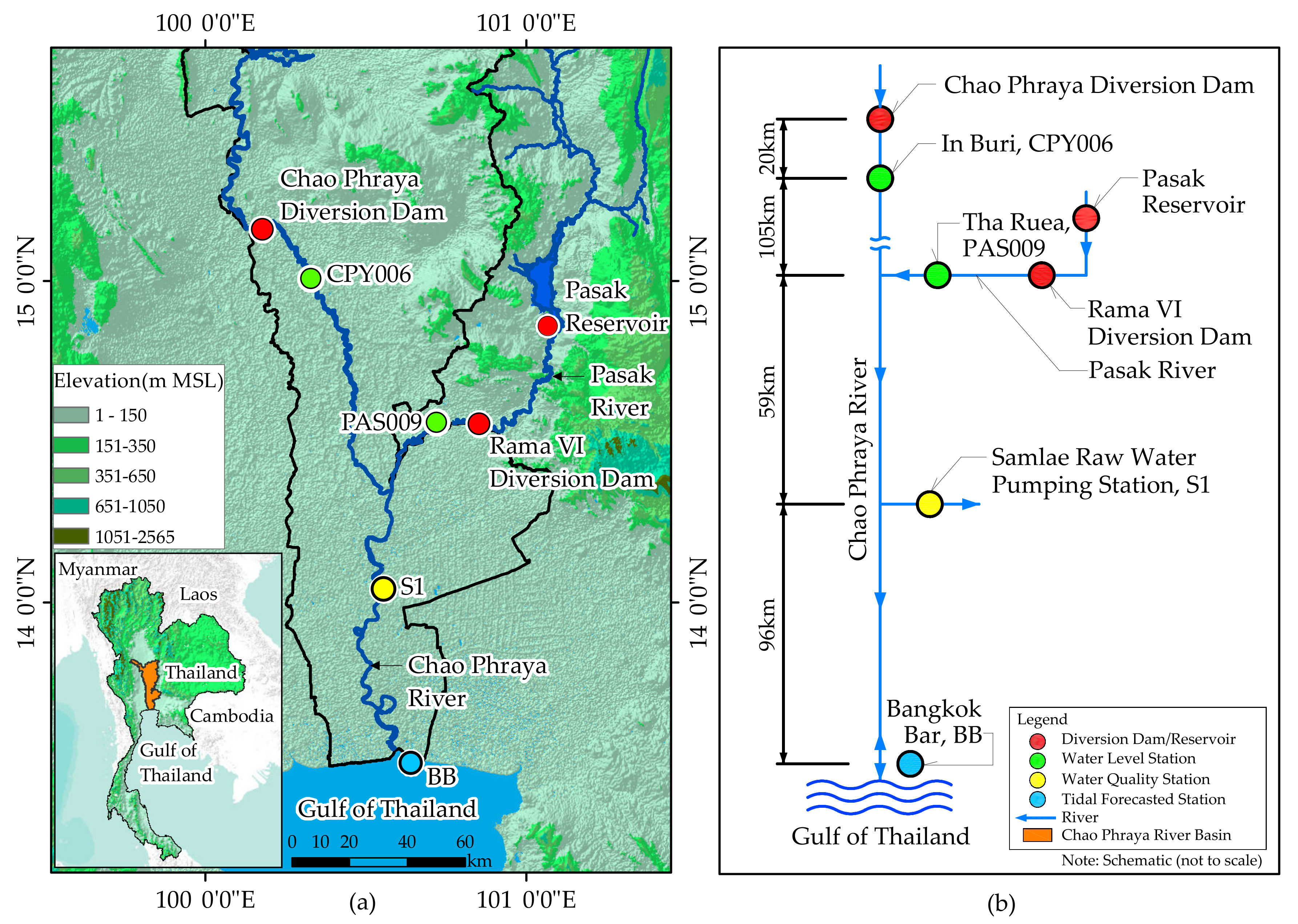
2.1. Study Site and Data Collection

The Samlae pumping station, which is a raw water pumping station that supplies water to Bangkok, is located 96 km upstream from the Chao Phraya’s mouth. Whenever the seawater intrudes up the Samlae pumping station, the water supply will have a high salinity level because water supply production processes do not include desalination. Since this study aims to forecast salinity in advance for warning purposes, salinity level at Samlae pumping station (S1) was chosen to be the target variable.

At the Samlae pumping station, the salinity was continuously measured in the river with water quality monitoring equipment. The device was the YSI 6600 V2 Sonde and the probe was well below the lowest water level at all time. The conductivity was continuously measured and converted to salinity hourly. According to the device specifications, the range of salinity was between 0 to 70 $\mathrm{g}$ ${\mathrm{L}}^{-1}$, the resolution was $0.01$ $\mathrm{g}$ ${\mathrm{L}}^{-1}$, and the accuracy was ±1% of reading or $0.1$ $\mathrm{g}$ ${\mathrm{L}}^{-1}$, whichever was greater.

Figure 1 shows locations of the measurement stations on both the map and the schematic diagram. Data of various variables judged (based on hydrology) to likely have an impact on the salinity level at the Samlae pumping station collected from multiple sources were selected to be candidates for the predictor variables. The candidate variables were the time-series data of salinity, water levels and forecasted tidal level at multiple measurement stations along the Chao Phraya river. The data sets were continuously measured along the Chao Phraya River by the following governmental organisations: the Metropolitan Waterworks Authority (MWA), the Hydro Informatics Institute (HII), and the Hydrographic Department, Royal Thai Navy (RTN). A preliminary analysis was conducted to narrow down the candidate predictor variables, and it was found that measurements of the same variable at different stations contained a high amount of mutual information. The analysis to find cross-correlation between multiple variables and the salinity at S1 suggested that four time-series variables should suffice for forecasting the salinity at the Samlae pumping station (S1), and these were: the salinity level itself, the water level at Inburi measurement station (CPY006), the water level at Tha Ruea measurement station (PAS009), and the forecasted tidal level at Bangkok Bar (BB).

This choice of time-series variables: CPY006, PAS009, and BB (and the salinity itself) was justified from a hydrological perspective. (i) CPY006 contained information about the Chao Phraya river’s discharge. It was also an indicator of the seawater flushing operation; (ii) PAS009 contained information about the impact of a principal tributary (Pasak River) to S1, which also indicated the flushing operation; and (iii) BB contained information about seawater intrusion at the Chao Phraya river mouth. All data sets had been continuously collected since 2014, however, there were some missing data. Although the river flow was an important factor affecting salinity and other water quality parameters in estuaries, however, we used the measured river flow depths at the CPY006 and PAS009 stations instead of the river flows because the river flows at both stations were the secondary variables computed from the depths using the stage-discharge rating curve.

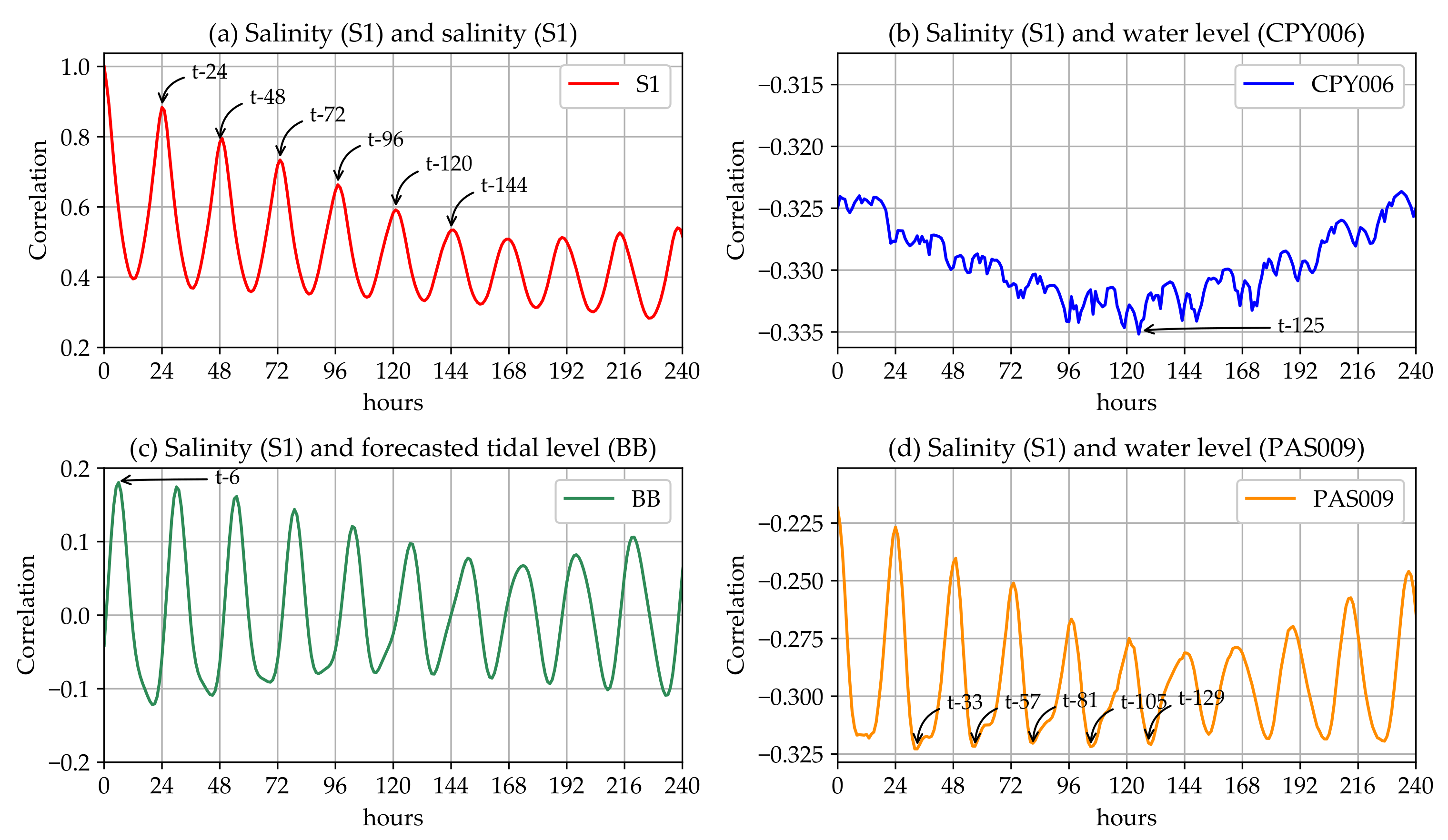
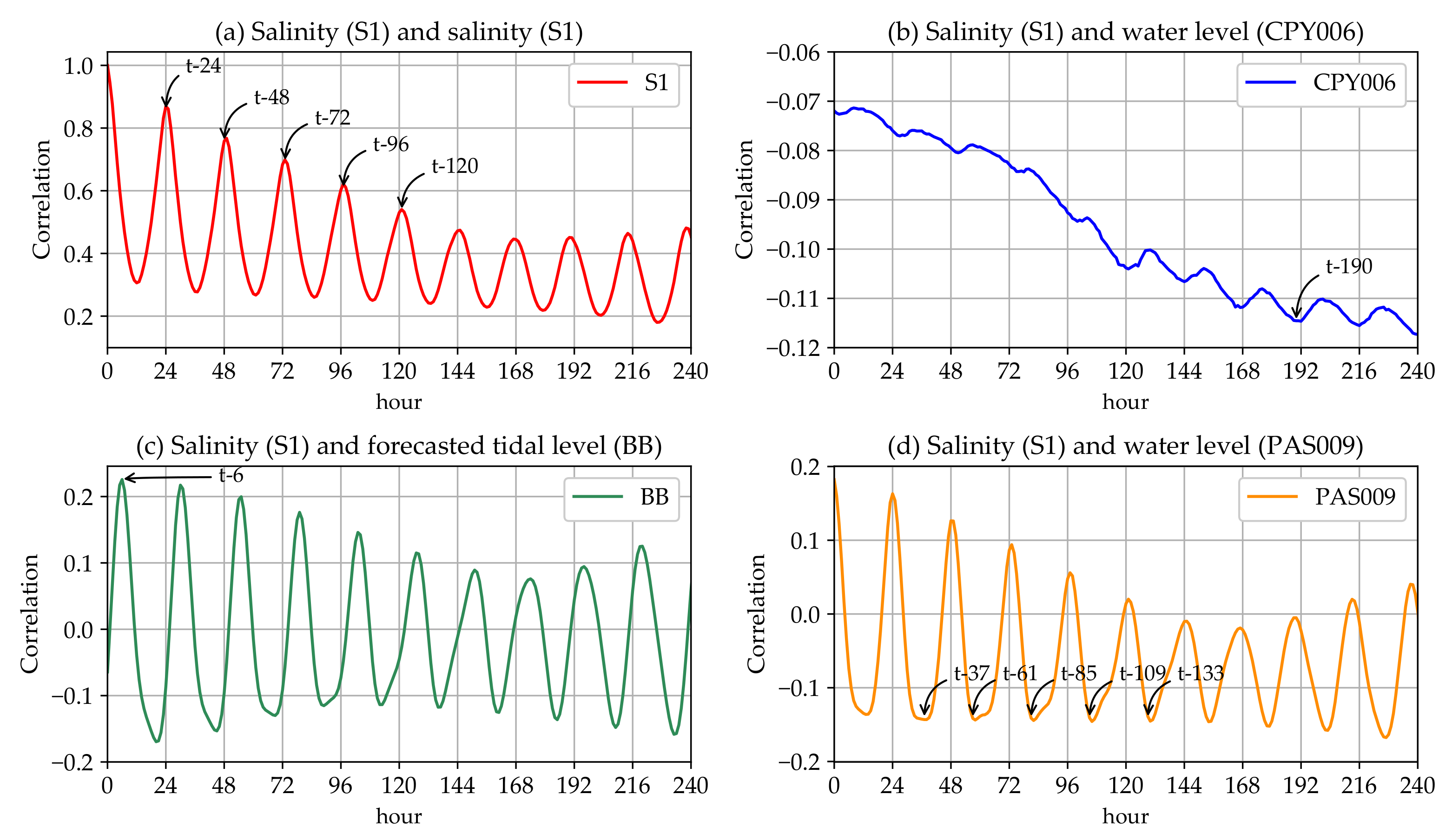
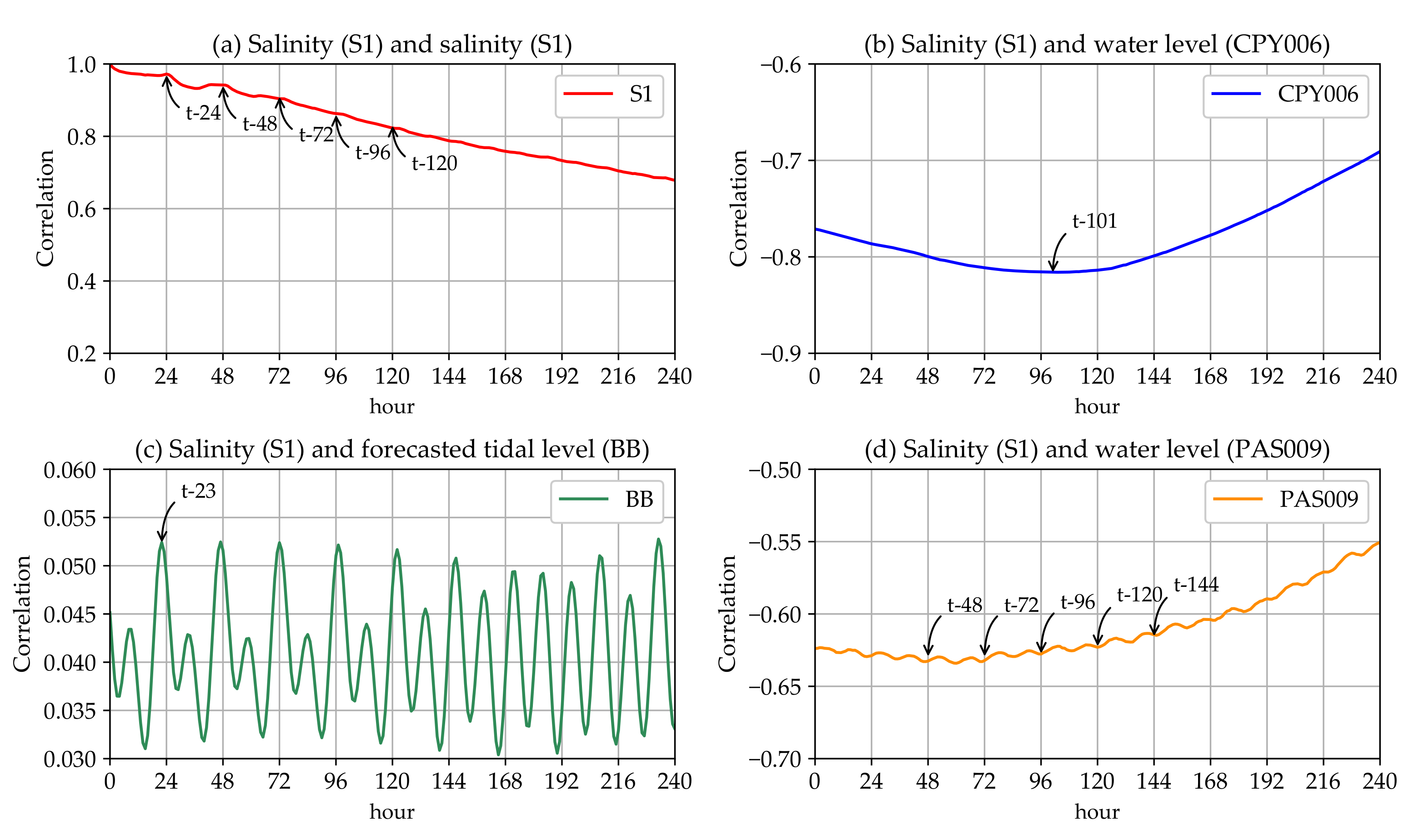
2.2. Selection of the Predictor Variables

Although we had already selected time-series to analyse, which were S1, CPY006, PAS009 and BB, we had not yet selected predictor variables from those time series. The predictor variables referred to the value at a point of a time-series at a certain time lag to the target variable. While we aimed to forecast salinity at various forecast periods, the predictor variables must be at the time lag longer than the forecast period, that is, to make a forecast at 24 h in advance, all predictor variable must be collected at least 24 h before the target variable. A cross-correlation analysis was therefore performed to help select the specific time lags from each time-series to become input variables. The Pearson’s correlation analysis was carried out as a measure of cross-correlation to find the impact of each variable on S1. The Pearson correlation coefficient (r) was calculated between each predictor variable from the training set at a time and S1 throughout the whole range. Krehbiel [24] presented criteria for the coefficient of correlation (r) to indicate the two variables had a linear relationship with each other. The correlation coefficient could be low as long as the number of data points was large.

In the preliminary analysis, we calculated the Pearson correlation on a trial-and-error basis between a number of variables, including water levels at different positions in the Chao Phraya River and the Pasak River, and the tidal forecast at the Chao Phraya mouth (BB). We found the water level at various points contained a lot of mutual information, and therefore, only a few variables should suffice for model construction. Thus, the selected variables for analysis were the water level at Inburi Station (CPY006), the tidal forecast at Bangkok Bar (BB), and the water level at Tha Ruea Station (PAS009). The cross-correlations between S1 and various variables are shown in Figure 2. The results of all four cross-correlation analyses showed periodic patterns with a period of 24 h which corresponded to the tide period. The auto-correlation of S1 had its peaks every 24 h with declining magnitude as the time lag increased. The cross-correlation between S1 and CPY006 showed a strong trend component with some seasonal patterns. The highest magnitude of the cross-correlation was when the time lag was 128 h. The correlation coefficients were negative throughout the time range, indicating that higher water level upstream at the Chao Phraya river corresponded to lower salinity at Samlae pumping station. The cross-correlation between S1 and BB also varied periodically, but it fluctuated around positive and negative values. Lastly, S1 and PAS009 were negatively correlated, with the cross-correlation result varying in a periodic pattern.

The predictor variables were selected from a point of time of each variable in the time-series. From the cross-correlation plots, the variables from the time-series at the peaks were selected subjected to the condition that the time lag had to be longer than the forecast period to provide realistic forecasting. After each variable had been selected from the time-series, various combinations of variables were chosen as candidate models for salinity forecasting (see Equations (1)–(3)). We then made a simple multiple linear regression model based on the least squares method. Residuals from the model were analysed graphically. Details of the residual analysis are discussed in Appendix A. The cross-correlation analysis demonstrated that the Pearson correlation coefficient (r) between S1 and S1 itself varied periodically, with local optima occurred at every 24 h. Similarly, a periodic trend was found in the cross-correlation between PAS009 and S1. These results implied tidal currents had an impact on the salinity level. The correlation coefficient between S1 and CPY006 had its highest magnitude at 125 h before the time of forecast, while the correlation coefficient between S1 and BB had its highest magnitude 6 h before the time of forecast. Based on these results, the optimal time lag for each predictor variable to forecast for S1 was selected.

For forecasting perspective, we aim to make a forecast at various forecast periods of 24 h, 48 h, 72 h, 96 h and 120 h in advance. Combinations of predictor variables were divided into 3 candidates, which are shown in Equation (1)–(3). The forecasting models would be trained and cross-validated with all candidates at various forecast periods. Model candidates for forecasting were

$$\begin{array}{cc}\mathrm{S}{1}_{\mathrm{t}}=\mathrm{f}(\mathrm{S}{1}_{\mathrm{t}-\mathrm{F}\mathrm{P}},\mathrm{S}{1}_{\mathrm{t}-\mathrm{F}\mathrm{P}-24},\mathrm{C}\mathrm{P}\mathrm{Y}{006}_{\mathrm{t}-125},\mathrm{B}{\mathrm{B}}_{\mathrm{t}-6},\mathrm{P}\mathrm{A}\mathrm{S}{009}_{\mathrm{t}-\mathrm{F}\mathrm{P}-9})\hfill & \hfill \mathrm{Candidate}1\mathrm{A}\end{array}$$

(1)

$$\begin{array}{cc}\mathrm{S}{1}_{\mathrm{t}}=\mathrm{f}(\mathrm{S}{1}_{\mathrm{t}-\mathrm{F}\mathrm{P}},\mathrm{S}{1}_{\mathrm{t}-\mathrm{F}\mathrm{P}-24},\mathrm{C}\mathrm{P}\mathrm{Y}{006}_{\mathrm{t}-125},\mathrm{B}{\mathrm{B}}_{\mathrm{t}-6})\hfill & \hfill \mathrm{Candidate}1\mathrm{B}\end{array}$$

(2)

$$\begin{array}{cc}\mathrm{S}{1}_{\mathrm{t}}=\mathrm{f}(\mathrm{S}{1}_{\mathrm{t}-\mathrm{F}\mathrm{P}},\mathrm{S}{1}_{\mathrm{t}-\mathrm{F}\mathrm{P}-24})\hfill & \hfill \mathrm{Candidate}1\mathrm{C}\end{array}$$

(3)

where S1 was the salinity at Samlae pumping station, CPY006 was the water level above the mean sea level at Inburi Station, PAS009 was the water level at Tha Ruea Station and BB was the predicted tidal level at Bangkok Bar Station. The subscripts refer to the time of the time-series, the subscript t denotes the time of forecast, the subscript FP denotes the forecast period; all units of time are in hours. The training/validation data set was randomly divided into a training set (80%) and a cross-validation set (20%). The process of model training and validation supported the selection of the most suitable predictor variables combinations for salinity forecasting (this was the so-called model selection process).

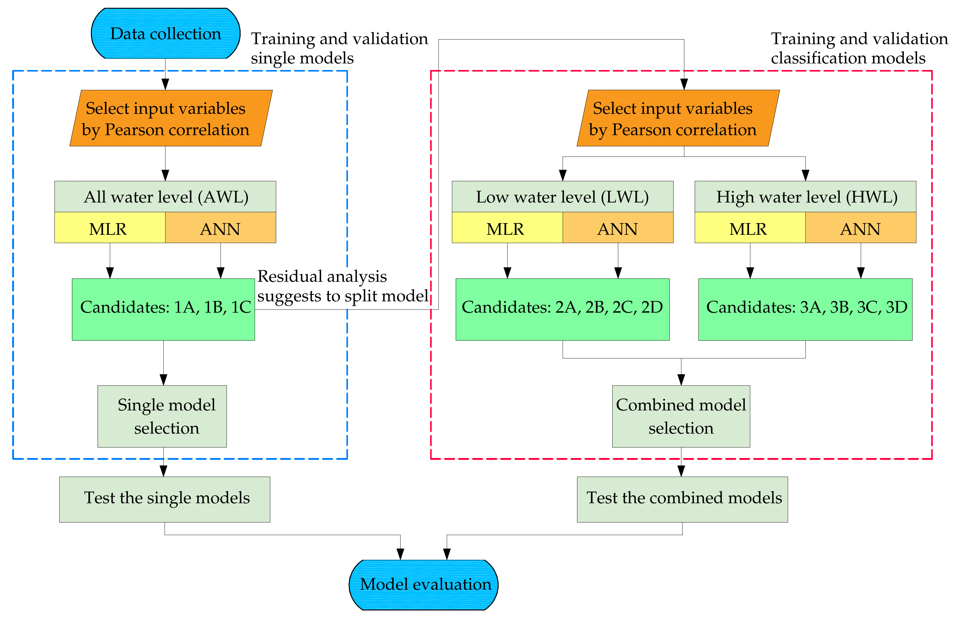
2.3. Model Development and Parameter Selection

We started developing models by using a simple MLR approach. Parameters were used according to candidates shown in Equation (1)–(3). The residuals from the trained models, which were the differences between the measurements and the forecasts, were graphically investigated (residual analysis). An MLR model assumes a linear relationship between the target variables and the predictor variables and works best when the residual is equal across all values of the independent variables. If the residual is highly heteroscedastic, it means the variability of a residual is unequal across the range of values of a variable that predicts it. In this case, the variability of the residuals was high when the water level at CPY006 was low and vice versa (See details in Appendix A). Hence, it indicated that the model could be consistent when the values of predictor variables were high, but it was highly inconsistent in accuracy when the values of predictor variables were low. To overcome this inconsistency, we proposed the use of two separate sub-models for forecasting: one when the water level was low and another when the water level was high. From observation of the residuals, the water level at CPY006 was a good model splitting boundary between the two sub-models. Therefore, the first sub-model explored was employed when the water level at CPY006 was lower than 4.0 m above mean sea level (MSL), that is, a low water level case (LWL) and the second sub-model was employed when the water level of CPY006 was higher than 4.0 m MSL, that is, a high water level case (HWL). The accuracy of the proposed combined-model method was investigated and compared with the single-model method afterward.

Once we decided to investigate the proposed concept of the combined model, which consisted of two sub-models, the model selection process was performed separately on each sub-model. The selection process included the cross-correlation analysis, the residual analysis from MLR results, and statistical analysis from MLR results. Details of the statistical analysis for parameter selections are shown here, where the model candidates for the low water level case (CPY006 < 4.0 m MSL) were

$$\begin{array}{cc}\mathrm{S}{1}_{\mathrm{t}}=\mathrm{f}(\mathrm{S}{1}_{\mathrm{t}-\mathrm{F}\mathrm{P}},\mathrm{C}\mathrm{P}\mathrm{Y}{006}_{\mathrm{t}-190},\mathrm{B}{\mathrm{B}}_{\mathrm{t}-6},\mathrm{P}\mathrm{A}\mathrm{S}{009}_{\mathrm{t}-\mathrm{F}\mathrm{P}-13})\hfill & \hfill \mathrm{Candidate}2\mathrm{A}\end{array}$$

(4)

$$\begin{array}{cc}\mathrm{S}{1}_{\mathrm{t}}=\mathrm{f}(\mathrm{S}{1}_{\mathrm{t}-\mathrm{F}\mathrm{P}},\mathrm{C}\mathrm{P}\mathrm{Y}{006}_{\mathrm{t}-190},\mathrm{B}{\mathrm{B}}_{\mathrm{t}-6})\hfill & \hfill \mathrm{Candidate}2\mathrm{B}\end{array}$$

(5)

$$\begin{array}{cc}\mathrm{S}{1}_{\mathrm{t}}=\mathrm{f}(\mathrm{S}{1}_{\mathrm{t}-\mathrm{F}\mathrm{P}},\mathrm{B}{\mathrm{B}}_{\mathrm{t}-6})\hfill & \hfill \mathrm{Candidate}2\mathrm{C}\end{array}$$

(6)

$$\begin{array}{cc}\mathrm{S}{1}_{\mathrm{t}}=\mathrm{f}\left(\mathrm{S}{1}_{\mathrm{t}-\mathrm{F}\mathrm{P}}\right)\hfill & \hfill \mathrm{Candidate}2\mathrm{D}\end{array}$$

(7)

Similarly, the model candidates for the high water level case (CPY006 > 4.0 m MSL) were

$$\begin{array}{cc}\mathrm{S}{1}_{\mathrm{t}}=\mathrm{f}(\mathrm{S}{1}_{\mathrm{t}-\mathrm{F}\mathrm{P}},\mathrm{C}\mathrm{P}\mathrm{Y}{006}_{\mathrm{t}-101},\mathrm{B}{\mathrm{B}}_{\mathrm{t}-23},\mathrm{P}\mathrm{A}\mathrm{S}{009}_{\mathrm{t}-\mathrm{F}\mathrm{P}-24})\hfill & \hfill \mathrm{Candidate}3\mathrm{A}\end{array}$$

(8)

$$\begin{array}{cc}\mathrm{S}{1}_{\mathrm{t}}=\mathrm{f}(\mathrm{S}{1}_{\mathrm{t}-\mathrm{F}\mathrm{P}},\mathrm{C}\mathrm{P}\mathrm{Y}{006}_{\mathrm{t}-101},\mathrm{P}\mathrm{A}\mathrm{S}{009}_{\mathrm{t}-\mathrm{F}\mathrm{P}-24})\hfill & \hfill \mathrm{Candidate}3\mathrm{B}\end{array}$$

(9)

$$\begin{array}{cc}\mathrm{S}{1}_{\mathrm{t}}=\mathrm{f}(\mathrm{S}{1}_{\mathrm{t}-\mathrm{F}\mathrm{P}},\mathrm{C}\mathrm{P}\mathrm{Y}{006}_{\mathrm{t}-101})\hfill & \hfill \mathrm{Candidate}3\mathrm{C}\end{array}$$

(10)

$$\begin{array}{cc}\mathrm{S}{1}_{\mathrm{t}}=\mathrm{f}\left(\mathrm{S}{1}_{\mathrm{t}-\mathrm{F}\mathrm{P}}\right)\hfill & \hfill \mathrm{Candidate}3\mathrm{D}\end{array}$$

(11)

For the combined model, the cross-correlation analysis results suggested a different time lag between predictor variables and the target variable than the time lag used for the single-model case. The cross-correlation between S1 and predictor variables for the low water level is shown in Figure 3 and for the high water level is shown in Figure 4. As can be observed, the behaviours of the cross-correlation between the variables differed for the low water level and the high water level. We therefore selected different points of the time-series to be predictor variables in the two cases.

We also trained the ANN models in parallel with the MLR models using the same input variables, as listed in Equations (1)–(11). The number of hidden layer we used was one, as suggested by the Ref. Zhou et al. [13], ASCE [21] and the activation function was the sigmoid function because it was one of the most common activation functions used in Salinity Forecasting [11,25,26] and in Water Quality Forecasting [27,28,29].

Furthermore, compared to the single model candidate equations, predictor variables for the combined-model case did not include S1 at forecast period minus 24 h before the time of forecast (subscript t-FP-24) because the coefficient of $\mathrm{S}{1}_{\mathrm{t}-\mathrm{F}\mathrm{P}-24}$ from MLR was much smaller than the term $\mathrm{S}{1}_{\mathrm{t}-\mathrm{F}\mathrm{P}}$. Additionally, the t-statistic of the hypothesis test indicated that the model was not significantly different with or without this term, that is, p-value > 0.05. A summary of all the processes for salinity forecasting is presented in Figure 5.

3. Results and Discussion

In this section, we describe how all the model candidates were compared and selected in both the single model and the combined-model cases. The model candidates were cross-validated using a 80/20 cross-validation split. The cross-validation results were compared through the performance indicators. Once the best model candidates had been selected, they were tested on continuous time series data from a period of two months. A salinity time-series data set for a period of two months had been reserved for testing. Those two months were April 2020, when seawater intrusion occurred heavily, that is, salinity exceeded the surveillance threshold of $0.25$ $\mathrm{g}$ ${\mathrm{L}}^{-1}$ and October 2020, when no seawater intrusion was observed. Additionally, an application of the model as an alarm system is demonstrated at the end of the section.

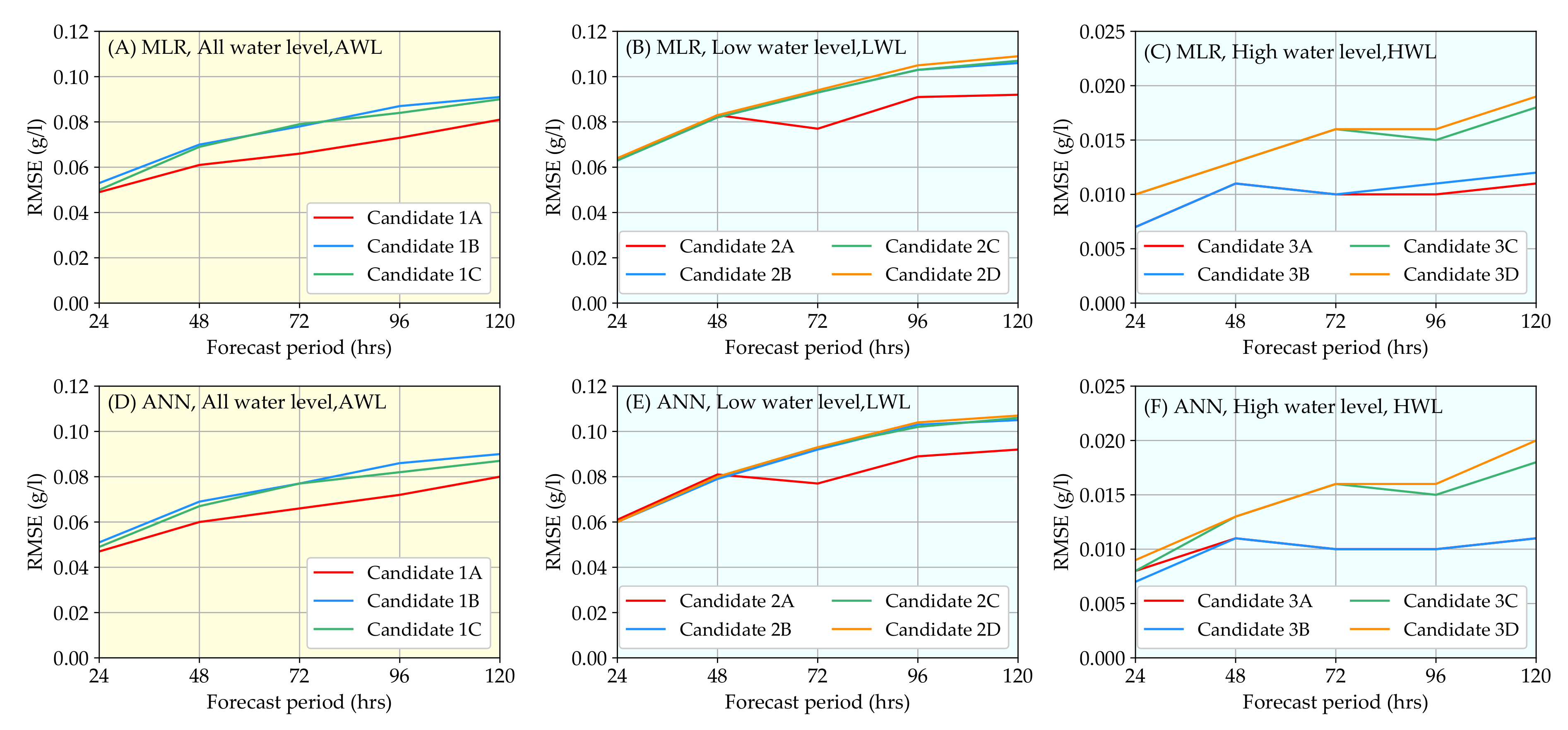
3.1. Model Performance Comparison and Validation

Since we already had a few of the model candidates for forecasting, we compared each candidate to select the best model for single-model forecasting and also to select the best model combination for the combined-model forecasting. We used three metrics to measure forecasting performance in the validation process, which were the coefficient of determination (${\mathrm{R}}^2$), the root mean squares of errors (RMSE) and the mean absolute percentage error (MAPE). To calculate all the performance indicators, we used a random 80/20 cross-validation split. The cross-validation was performed three times and then the MLR coefficients were averaged in each candidate for each forecast period to guarantee the consistency of the models. Detailed results of the cross-validation can be found in the Appendices. The values of ${\mathrm{R}}^2$ indicated that for every model candidate, there was a strong relationship between the dependent variable and the independent variables.

The values of the RMSE and the MAPE are important performance indicators for forecasting. The RMSE was chosen as a main indicator to select the best models. The best models for both the single-model case and combined-model case were later used in the testing period. The comparison of the RMSE between each case is shown in Figure 6. In each plot, the RMSE for various model candidates at various times of forecast are compared. The fit type (whether it was ANN or MLR) and the model cases (all water level (AWL) for the single model, and low water level (LWL) and high water level (HWL) for the combined model) is clearly stated on each sub-plot.

Figure 6 shows that the results of models fitted by MLR was not significantly different to those fitted by ANN. The RMSE gradually increased as the time of forecast increased from 24 h to 120 h in advance. The RMSE rose from $0.05$ $\mathrm{g}$ ${\mathrm{L}}^{-1}$ to $0.09$ $\mathrm{g}$ ${\mathrm{L}}^{-1}$ for the single-model case, whereas the range of the RMSE for the combined model was different for each sub-model. The RMSE varied from $0.06$ $\mathrm{g}$ ${\mathrm{L}}^{-1}$ to $0.11$ $\mathrm{g}$ ${\mathrm{L}}^{-1}$ for the LWL sub-model and from only $0.005$ $\mathrm{g}$ ${\mathrm{L}}^{-1}$ to $0.02$ $\mathrm{g}$ ${\mathrm{L}}^{-1}$ for the HWL sub-model. This difference in the RMSE for each sub-model was evidence that the relationship between the forecast and the predictor variables changed between the two cases. Patterns similar to the RMSE were also observed on the ${\mathrm{R}}^2$ and the MAPE.

The model performance was compared to select the best candidates for both the single model and the combined model using the RMSE as the performance indicator. In the single-model case, candidate 1A outperformed candidates 1B and 1C as the RMSE from candidate 1A was lower at all times of the forecast. This was also true with both the MLR or the ANN. In the LWL case of the combined model, candidate 2A yielded the lowest RMSE among other candidates regardless of fit type (MLR or ANN). In the HWL case of the combined model, candidates 3A and 3B provided almost identical RMSE, which was lower than that of candidates 3C and 3D.

Thus, the best-performing model for each case was selected to test against continuous data in Section 3.2. The selected candidates with variables for each case are shown in

Table 1. The selected model candidates for different cases from the RMSE.

Model	Case	Candidate
		MLR	ANN
Single model	AWL	1A: Equation (1)	1A: Equation (1)
Combined model	LWL	2A: Equation (4)	2A: Equation (4)
	HWL	3A: Equation (8)	3B: Equation (9)

.

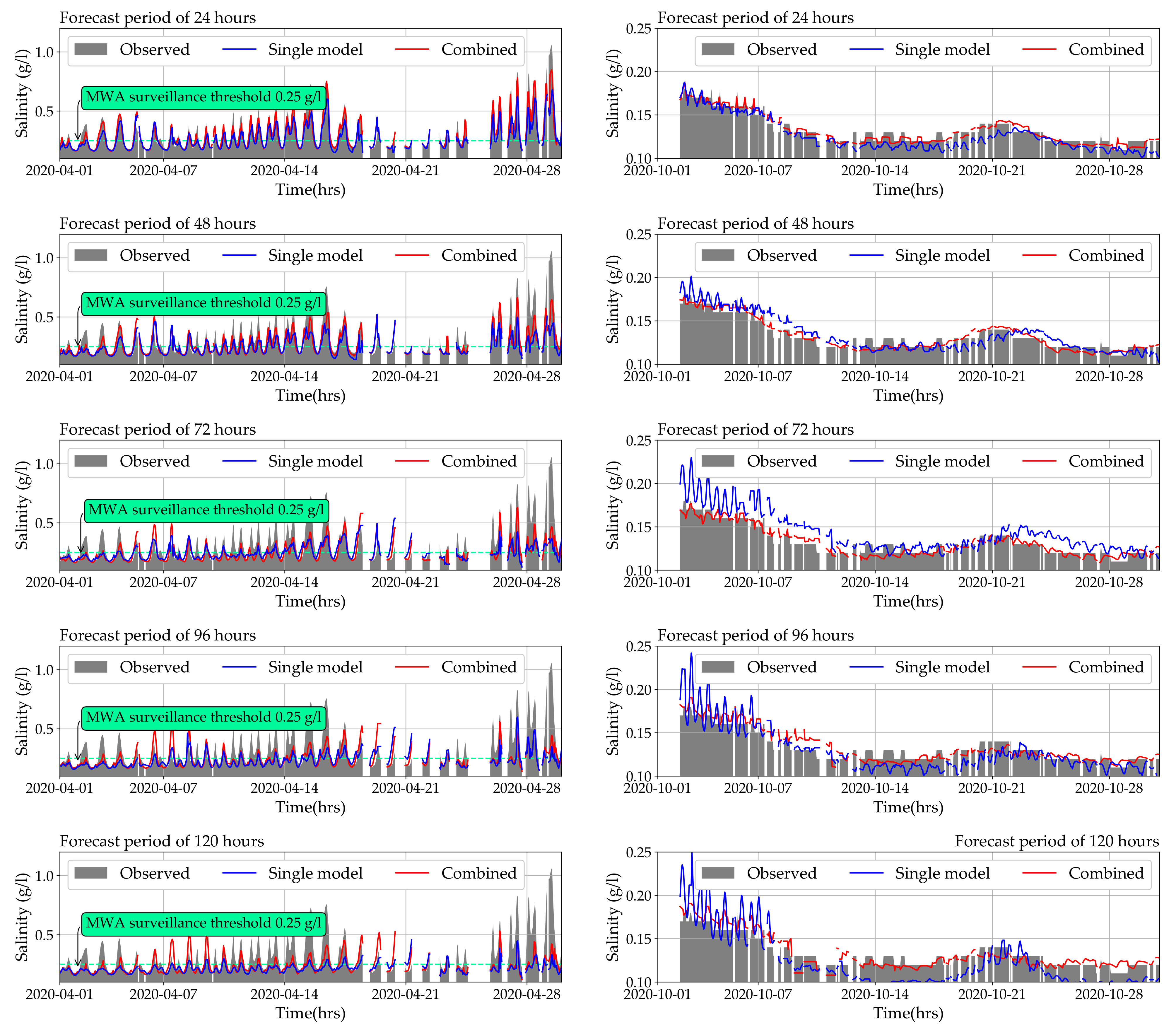
3.2. Model Test: Comparing Continuous Forecasting with Real Data

In this section, we illustrate the use of selected models to continuously forecast the salinity. Two data sets with a period of one month each were selected as testing data sets. These two data sets had been reserved for model testing and was not included in the model selection and validation processes. The first data set was from April 2020, when salinity intrusion occurred heavily, while the second data set was from October 2020, when salinity intrusion did not exceed the surveillance threshold of $0.25$ $\mathrm{g}$ ${\mathrm{L}}^{-1}$.

In the testing period, we also used the Nash–Sutcliffe efficiency (NSE) to evaluate model performance. Those two months are April 2020, when seawater intrusion occurred heavily, that is, salinity exceeded the surveillance threshold of $0.25$ $\mathrm{g}$ ${\mathrm{L}}^{-1}$ and October 2020, when no excessive seawater intrusion was observed.

The continuous forecast as a result of model testing is illustrated in Figure 7. While the continuous forecast was carried out using both the ANN and the MLR, Figure 7 showed the forecast through the ANN model candidates in Table 1 as they performed slightly better than the MLR. Missing data were observed occasionally in the testing period. Subplots on the left column represent the continuous forecast on April 2020, while those on the right column represent October 2020. The time of forecast varied from 24 h to 120 h from top to bottom. Each subplot consists of the observed salinity, the forecasts using the single model and the forecasts using the combined model. Overall, the accuracy of the forecast decreased as the time of forecast increased. This agreed with the results from model validation. On April 2020, at 24–48 h forecast period, the combined model was able to capture high peaks of salinity slightly better than the single model. However, when the time of forecast was longer, the combined model sometimes forecasted peaks which were not observed in the real data. On October 2020, at 24–48 h forecast period, both models performed similarly. Nevertheless, as the forecast period increased, the forecasts from the single model fluctuated, which was inconsistent with the real data.

Performance of both models on forecasting was evaluated numerically and is shown in

Table 2. The performance evaluation of the single model. Units of the RMSE and the MAPE are gram per litres and percent respectively.

Forecast Period (h)	MLR				ANN
	${\mathbf{R}}^2$	RMSE	MAPE	NSE	${\mathbf{R}}^2$	RMSE	MAPE	NSE
24	0.860	0.073	10.487	0.776	0.865	0.069	10.327	0.796
48	0.741	0.099	14.975	0.585	0.735	0.096	12.150	0.605
72	0.530	0.115	18.886	0.416	0.576	0.110	16.255	0.469
96	0.412	0.120	19.731	0.299	0.460	0.119	16.100	0.319
120	0.365	0.113	21.556	0.272	0.448	0.111	18.280	0.290

and

Table 3. The performance evaluation of the combined model. Units of the RMSE and the MAPE are gram per litres and percent respectively.

Forecast Period (h)	MLR				ANN
	${\mathbf{R}}^2$	RMSE	MAPE	NSE	${\mathbf{R}}^2$	RMSE	MAPE	NSE
24	0.888	0.058	8.131	0.853	0.892	0.054	7.671	0.875
48	0.734	0.091	13.177	0.643	0.748	0.085	11.168	0.687
72	0.583	0.108	14.922	0.480	0.599	0.104	13.624	0.514
96	0.449	0.120	16.249	0.338	0.493	0.111	15.531	0.434
120	0.392	0.117	16.797	0.283	0.448	0.107	16.172	0.395

. Overall, the accuracy decreased as the forecast period increased. This decrease in accuracy was captured by all performance indicators, which are ${\mathrm{R}}^2$, RMSE, MAPE and NSE. The RMSE was the lowest at $0.054$ $\mathrm{g}$ ${\mathrm{L}}^{-1}$ for the 24 h forecast period using the combined model fitted with ANN, whereas the RMSE was the highest at $0.117$ $\mathrm{g}$ ${\mathrm{L}}^{-1}$ for the 120 h forecast period using the combined model fitted with MLR. Comparing between the two model fit types, the accuracy of the forecasting performed through the ANN was slightly better than that performed through the MLR. The difference in accuracy between those fit types lied in the third decimal digit in RMSE in the unit of gram per litre.

Lastly, the combined model outperformed the single model at all forecast periods regardless of the fit type. This was because each sub-model in the combined model better captured the physical factors that were different between when the water level was high and when the water level was low. The improvement in the Nash–Sutchliffe efficiency of the combined model over the single model is presented in

Table 4. The improvement of the combined model compared to the single model.

Forcast Period (h)	MLR	ANN
24	9.03%	9.03%
48	9.02%	11.94%
72	13.33%	8.75%
96	11.54%	26.50%
120	3.89%	26.58%

.

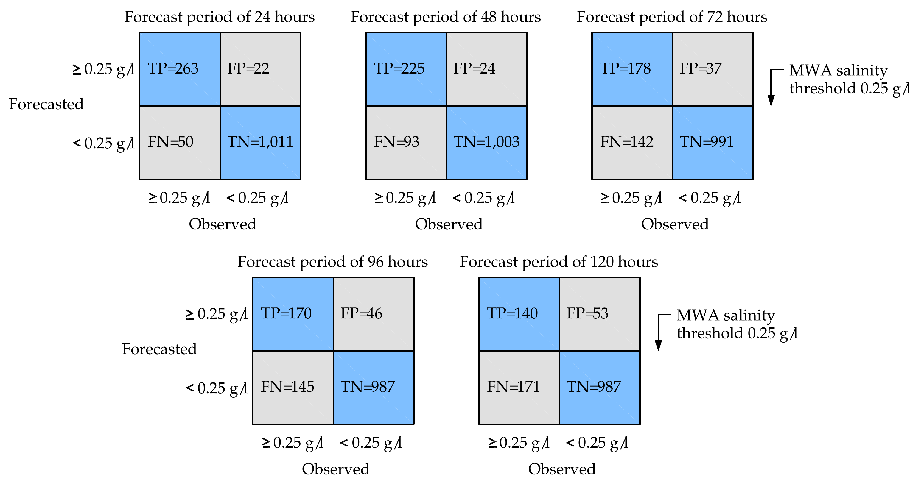
3.3. An Application of the Model as an Alarm System

Up to this point, models have been developed, cross-validated and tested against real data with continuous forecasting.

In this section, we will outline how the models can be used as a basis for an Alarm System. Such an alarm system would be of huge benefit to the waterworks authority in their operational planning and management as they would be able to schedule the pumping stations to minimise the effects of saltwater intrusion.

Here, a simple classification problem is formulated from the forecast and the measurement of the salinity. A confusion matrix, which summarises forecasting results on a classification problem is employed. The number of correct and incorrect forecasts are summarised with count values broken down by class. We use a binary confusion matrix and the MWA’s salinity threshold of $0.25$ $\mathrm{g}$ ${\mathrm{L}}^{-1}$ to evaluate the results of the salinity forecasts at Samlae raw water pumping station. The criteria are thus defined as follows:

Case 1:

Observed salinity ≥ 0.25 $\mathrm{g}$ ${\mathrm{L}}^{-1}$, and forecasted salinity ≥ 0.25 $\mathrm{g}$ ${\mathrm{L}}^{-1}$ is true positive (TP);

Case 2:

Observed salinity ≥ 0.25 $\mathrm{g}$ ${\mathrm{L}}^{-1}$, and forecasted salinity < 0.25 $\mathrm{g}$ ${\mathrm{L}}^{-1}$ is false negative (FN);

Case 3:

Observed salinity < 0.25 $\mathrm{g}$ ${\mathrm{L}}^{-1}$, and forecasted salinity < 0.25 $\mathrm{g}$ ${\mathrm{L}}^{-1}$ is true negative (TN);

Case 4:

Observed salinity < 0.25 $\mathrm{g}$ ${\mathrm{L}}^{-1}$, and forecasted salinity ≥ 0.25 $\mathrm{g}$ ${\mathrm{L}}^{-1}$ is false positive (FP).

Four indicators are used to quantitatively evaluate the forecasting performance, namely, the accuracy, the sensitivity, the specificity and the Matthews correlation coefficient (MCC). The accuracy indicates the overall accuracy of classification. The sensitivity (true positive rate) estimates the proportion of correctly identified positive forecasts. The specificity (true negative rate) measures the proportion of correctly identified negative forecasts. The MCC evaluates the performance of models based on the correlation rate between observed salinity and forecasted salinity. The MCC ranges between −1 to 1, where −1 indicates perfect disagreement between observed salinity and forecasted salinity and 1 indicates perfect agreement [30].

According to the model validation and testing processes, the combined model outperforms the single model and the ANN provides better forecasting results than MLR. Therefore, we use the forecasting results from the combined model fitted through an ANN as the predictor and evaluate its performance with the binary confusion matrix. The confusion matrices at various forecast periods are shown in Figure 8 and the performance indicators for the confusion matrices are summarised in

Table 5. The forecast performance evaluated through the confusion matrix.

Forecast Period (h)	Accuracy	Sensitivity (True Positive Rate)	Specificity (False Positive Rate)	MCC
24	0.947	0.840	0.979	0.847
48	0.913	0.708	0.977	0.748
72	0.867	0.556	0.964	0.605
96	0.858	0.540	0.955	0.571
120	0.834	0.450	0.949	0.480

. As one might expect, all performance indicators decrease when the forecast period increases. The 24 h forecast period has the highest accuracy, 0.947. The accuracy gradually decreases to 0.834 as the forecast period goes to 120 h. The true positive rate (sensitivity), however, drops much faster from 0.840 at 24 h forecast period to 0.450 at 120 h forecast period. In contrast, the true negative rate (specificity) does not change much at various forecast times. Lastly, the MCC shows identical trends to the sensitivity with the highest value of 0.847 when the forecast is performed 24 h in advance and 0.480 when the forecast is performed 120 h in advance.

4. Conclusions

In summary, saltwater intrusion negatively affects the lives of people in the lower Chao Phraya river area; in particular, it affects the raw water in the MWA’s water distribution network in that area, since raw water is pumped from the Chao Phraya River.

Currently, relocation of the pumping station is probably the most suitable long-term solution, however, a short- to middle-term solution is also required. This study presented data-driven methods to forecast salinity at the raw water pumping station for MWA water supply networks, Thailand. These methods will be greatly beneficial to MWA operational management, especially when saltwater intrusion occurs. The results show that the salinity can be forecasted accurately in advance from 1 to 5 days. The whole model development process has been described in detail throughout this paper; this study contained some interesting findings, as follows:

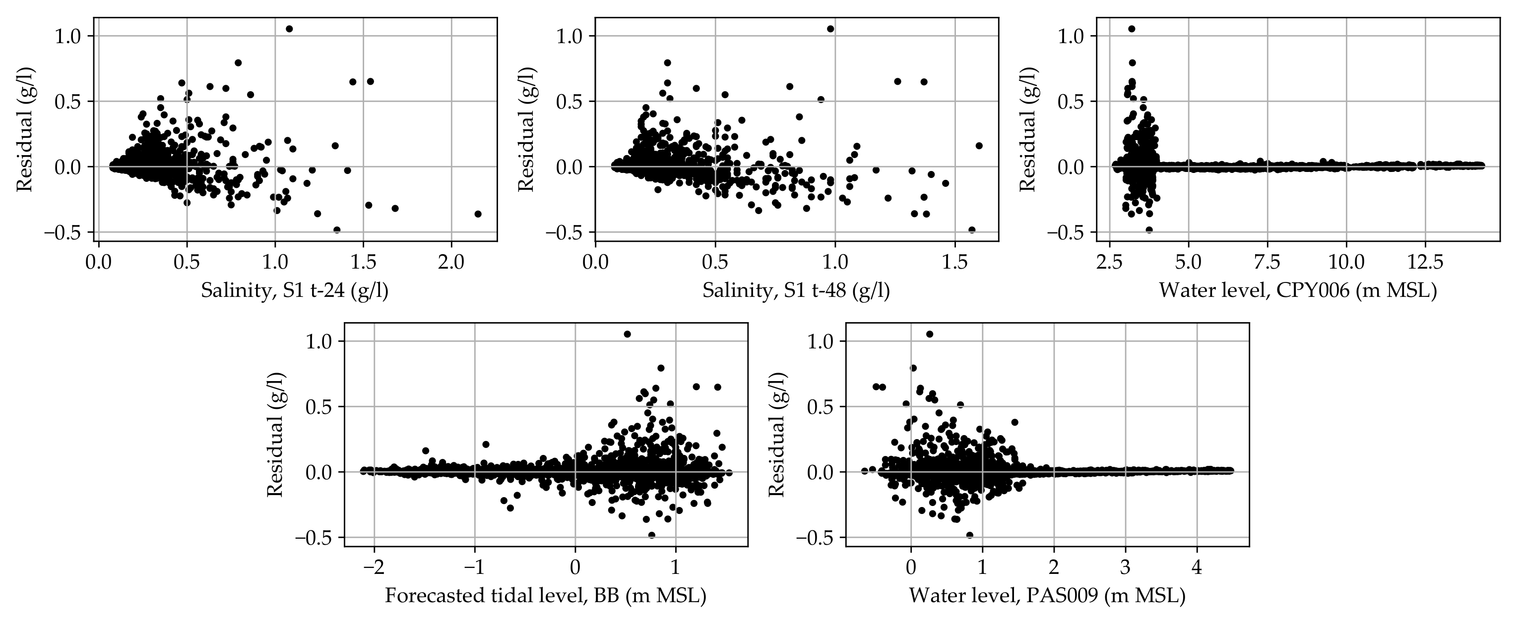
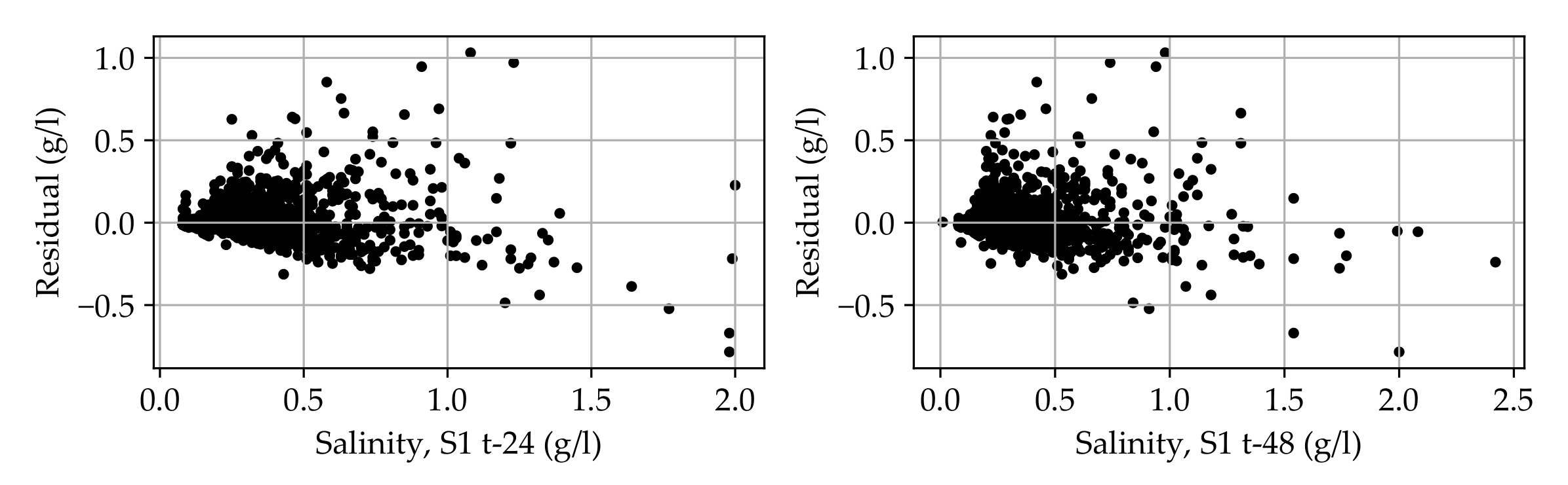
• The residual analysis of the the multiple linear regression (MLR) indicated that the model behaviours were different at high and low water levels, therefore, a two-stage model (the combined model) was proposed, analysed and compared to the single model;
• Two model fitting methods, which were the MLR and the artificial neuron network (ANN), were investigated;
• The combined model using MLR and ANN performed better than single models in forecasting hourly salinity at 24 to 120 h;
• When the forecast period increased from 24 to 120 h, the forecasting performances of all the models decreased rapidly. Still, the combined model performed better than the single model in all cases;
• The forecasting model can be effectively utilized as an alarm system. The confusion matrix shows the performance of the alarm system for early warning of a saltwater intrusion event at various forecast periods. The accuracy decreases as the forecast periods increases. In practice, a suitable forecast period can be selected based on the user’s needs.

This study showed that data-driven models, such as multiple linear regression (MLR) and the artificial neural network (ANN) can effectively be used for river salinity forecasting. Thus, they can form the basis of a salt water intrusion early-warning system for the Metropolitan Waterworks Authority, which would allow them to schedule their raw water pumping schedule more effectively.

References

- World Health Organization. Acceptable aspects: Taste, Odour and Appearance. Guidelines for Drinking-Water Quality, 4th ed.; Incorporating the 1st Addendum; World Health Organization: Geneva, Switzerland, 2008; pp. 219–230. [Google Scholar]
- Chong, Y.J.; Khan, A.; Scheelbeek, P.; Butler, A.; Bowers, D.; Vineis, P. Climate change and salinity in drinking water as a global problem: Using remote-sensing methods to monitor surface water salinity. Int. J. Remote Sens. 2014, 35, 1585–1599. [Google Scholar] [CrossRef]
- Kaushal, S.S. Increased salinization decreases safe drinking water. Environ. Sci. Technol. 2016, 50, 2765–2766. [Google Scholar] [CrossRef] [PubMed]
- Lassiter, A. Rising seas, changing salt lines, and drinking water salinization. Curr. Opin. Environ. Sustain. 2021, 50, 208–214. [Google Scholar] [CrossRef]
- Intaboot, N.; Taesombat, W. A Study of the Calibration of Salinity Dispersion in the Thachin Estuarine. In Proceedings of the 5th International Symposium on Fusion of Science and Technology (ISFT), New Delhi, India, 18–22 January 2016; pp. 101–105. [Google Scholar]
- Lam, N.T. Real-Time Prediction of Salinity in the Mekong River Delta. In Proceedings of the 10th International Conference on Asian and Pacific Coasts (APAC 2019), Hanoi, Vietnam, 25–28 September 2019; pp. 1461–1468. [Google Scholar]
- Alizadeh, M.J.; Kavianpour, M.R. Development of wavelet-ANN models to predict water quality parameters in Hilo Bay, Pacific Ocean. Mar. Pollut. Bull. 2015, 98, 171–178. [Google Scholar] [CrossRef]
- Alizadeh, M.J.; Kavianpour, M.R.; Danesh, M.; Adolf, J.; Shamshirband, S.; Chau, K.W. Effect of river flow on the quality of estuarine and coastal waters using machine learning models. Eng. Appl. Comput. Fluid Mech. 2018, 12, 810–823. [Google Scholar] [CrossRef]
- Melesse, A.M.; Khosravi, K.; Tiefenbacher, J.P.; Heddam, S.; Kim, S.; Mosavi, A.; Pham, B.T. River water salinity prediction using hybrid machine learning models. Water 2020, 12, 2951. [Google Scholar] [CrossRef]
- Jin, T.; Cai, S.; Jiang, D.; Liu, J. A data-driven model for real-time water quality prediction and early warning by an integration method. Environ. Sci. Pollut. Res. 2019, 26, 30374–30385. [Google Scholar] [CrossRef]
- Huang, W.; Foo, S. Neural network modeling of salinity variation in Apalachicola River. Water Res. 2002, 36, 356–362. [Google Scholar] [CrossRef]
- Hu, J.; Liu, B.; Peng, S. Forecasting salinity time series using RF and ELM approaches coupled with decomposition techniques. Stoch. Environ. Res. Risk Assess. 2019, 33, 1117–1135. [Google Scholar] [CrossRef]
- Zhou, F.; Liu, B.; Duan, K. Coupling wavelet transform and artificial neural network for forecasting estuarine salinity. J. Hydrol. 2020, 588, 125127. [Google Scholar] [CrossRef]
- Horiuchi, Y.; Matsuura, T.; Tebakari, T.; Wongsa, S. Meta-analysis of Water Quality Characteristics in the Lower Chaophraya River, Thailand. In Proceedings of the 22nd IAHR-APD Congress 2020, Sapporo, Japan, 14–17 September 2020. [Google Scholar]
- Wongsa, S. Impact of climate change on water resources management in the lower Chao Phraya Basin, Thailand. J. Geosci. Environ. Prot. 2015, 3, 53. [Google Scholar] [CrossRef]
- Sriratana, L.; Bisalyaputra, K. Reconnaissance Study on Saltwater Intrusion Control at Main Raw Water Pumping Station of Metropolitan Waterworks Authority (Thailand). Int. J. Eng. Technol. 2019, 11, 33–38. [Google Scholar] [CrossRef]
- Wang, Q.; Wang, S. Machine learning-based water level prediction in Lake Erie. Water 2020, 12, 2654. [Google Scholar] [CrossRef]
- Quilty, J.; Adamowski, J. Addressing the incorrect usage of wavelet-based hydrological and water resources forecasting models for real-world applications with best practices and a new forecasting framework. J. Hydrol. 2018, 563, 336–353. [Google Scholar] [CrossRef]
- Keskin, T.E.; Düğenci, M.; Kaçaroğlu, F. Prediction of water pollution sources using artificial neural networks in the study areas of Sivas, Karabük and Bartın (Turkey). Environ. Earth Sci. 2015, 73, 5333–5347. [Google Scholar] [CrossRef]
- Rajaee, T.; Khani, S.; Ravansalar, M. Artificial intelligence-based single and hybrid models for prediction of water quality in rivers: A review. Chemom. Intell. Lab. Syst. 2020, 200, 103978. [Google Scholar] [CrossRef]
- ASCE. Artificial neural networks in hydrology. I: Preliminary concepts. Chemom. Intell. Lab. Syst. 2000, 5, 115–123. [Google Scholar]
- Haddad, K.; Zaman, M.; Rahman, A.; Shrestha, S. Regional flood modelling: Use of Monte Carlo cross-validation for the best model selection. In World Environmental and Water Resources Congress 2010: Challenges of Change; ASCE: Reston, VA, USA, 2010; pp. 2831–2840. [Google Scholar]
- Nwanganga, F.; Chapple, M. Practical Machine Learning in R; John Wiley & Sons: Hoboken, NJ, USA, 2020. [Google Scholar]
- Krehbiel, T.C. Correlation coefficient rule of thumb. Decis. Sci. J. Innov. Educ. 2004, 2, 97–100. [Google Scholar] [CrossRef]
- Le, D.; Huang, W.; Johnson, E. Neural network modeling of monthly salinity variations in oyster reef in Apalachicola Bay in response to freshwater inflow and winds. Neural. Comput. Appl. 2019, 31, 6249–6259. [Google Scholar] [CrossRef]
- Qi, S.; Bai, Z.; Ding, Z.; Jayasundara, N.; He, M.; Sandhu, P.; Seneviratne, S.; Kadir, T. Enhanced Artificial Neural Networks for Salinity Estimation and Forecasting in the Sacramento-San Joaquin Delta of California. J. Water Resour. Plan. Manag. 2021, 147, 04021069. [Google Scholar] [CrossRef]
- Palani, S.; Liong, S.Y.; Tkalich, P. An ANN application for water quality forecasting. Mar. Pollut. Bull. 2008, 56, 1586–1597. [Google Scholar] [CrossRef] [PubMed]
- Sha, J.; Li, X.; Zhang, M.; Wang, Z.L. Comparison of Forecasting Models for Real-Time Monitoring of Water Quality Parameters Based on Hybrid deep-learning Neural Networks. Water 2021, 13, 1547. [Google Scholar] [CrossRef]
- EL Hamidi, M.J.; Larabi, A.; Faouzi, M. Numerical Modeling of Saltwater Intrusion in the Rmel-Oulad Ogbane Coastal Aquifer (Larache, Morocco) in the Climate Change and Sea-Level Rise Context (2040). Water 2021, 13, 2167. [Google Scholar] [CrossRef]
- Rong, G.; Li, K.; Han, L.; Alu, S.; Zhang, J.; Zhang, Y. Hazard Mapping of the Rainfall–Landslides Disaster Chain Based on GeoDetector and Bayesian Network Models in Shuicheng County, China. Water 2020, 12, 2572. [Google Scholar] [CrossRef]