Upscaling of Surface Water and Groundwater Interactions in Hyporheic Zone from Local to Regional Scale

Abstract

The groundwater (GW) and surface water (SW) interaction (SW-GW) through the hyporheic zone is a significant component in sustainable water resource management. The complexities in SW-GW interactions increase from a local to a regional scale and are affected by variation in hydraulic, hydrologic, and hydrogeologic (3H) processes. Controlling factors and their upscaling of these processes to assess SW-GW interaction have not been addressed sufficiently in previous studies. Additionally, it is unclear what the effective factors are at different scales during the upscaling. Therefore, the present review focused on controlling factors of 3H processes in SW-GW interaction and their upscaling techniques. Relevancy of controlling factors was identified at different scales. Applications of different approaches and their uncertainties were also discussed for the characterization of SW-GW interactions. The study revealed that the improved data from different approaches is crucial for machine learning training and its application in the SW and GW assessment at local, sub-catchment, and catchment scales. Based on the outcomes, a framework has been proposed to execute modalities of controlling factors using remote sensing, geophysics, and artificial intelligence. The proposed framework could help in handling big data and accurate upscaling for water resource management.

1. Introduction

The surface and subsurface hydrological exchanges through sediments between near-channel and in-channel water are known as a hyporheic zone (HZ) [1]. The HZ plays a crucial role in the depletion of dissolved contaminants in channel water, supply nutrients, and energy cycle to river ecology. It provides food for biological communities and controls Spatio-temporal pollutant transport in river water [2]. Understanding complex processes in the HZ due to variation in climate, topography, and geology are necessary to understand surface water-groundwater (SW-GW) interaction and their controlling factors for sustainable water resource management.

SW-GW interaction in the HZ is associated with different spatial scales, which do not have any universally accepted definition [3]. For instance, the hyporheic scale varies from 1 to 100 m refers to the transition zone of hyporheic flow (HF). The reach or local scale, dominated by GW flow conditions, varies between 100 and 1000 m or slightly greater than 1000 m. The sub-catchment scale, dominated by GW flow conditions of several streams, lies between the local scale and the catchment scale. The catchment scale is more than several kilometers, dominated by regional flows [3,4,5]. Due to complexities in SW-GW interaction, smaller-scale factors become irrelevant or less relevant at a larger scale [5]. Determination of a Spatio-temporal SW-GW interaction for a particular setting is a challenging task that is controlled by several factors such as type of SW body, geomorphological, hydrological, topographical, geological, chemical, biological, ecological, and climatological factors [6]. Interpolation of these factors from a small scale to a large scale is also a challenging task [7].

Recent studies focused on the upscaling of various controlling factors of SW-GW interaction from a point or local scale to a regional scale [8,9,10,11,12]. The key findings of some studies are summarized in

Table 1. Summary of recent studies for upscaling of various controlling factors of surface water-groundwater (SW-GW) interaction.

Reference	Key Findings
Vermeulen et al. [13]	Upscaled hydraulic conductivity and transmissivity in fine and coarse resolution mesh using different techniques.
Jana & Mohanty [14]	Upscaled soil hydraulic parameters and topographic conditions in a fine mesh.
Pryshlak et al. [15]	Upscaled hydraulic conductivity, channel morphology, and soil heterogeneity
Schmadel et al. [16]	Developed a framework to assess diel hydrologic fluctuations to hyporheic exchange in the absence of geomorphic complexity.
Di Ciacca et al. [8]	Used hydraulic conductivity of an aquifer and streambed properties to assess SW-GW interaction in a regional hydrogeological model.
Glose et al. [10]	Upscaled hydraulic conductivity using a different parameter termed vertically integrated hydraulic conductivity.
Magliozzi et al. [17]	Applied a statistical method in several factors of catchment scale, sub-catchment scale, and reach scale to identify potential areas of hyporheic exchange for river restoration planning.
Snowdon et al. [11]	Used topographic indices, hydraulic heads, and hyporheic exchange flux for groundwater resource management at different spatial scales.
Bastani & Harter [12]	Worked on the impact of temporal resolution upscaling of groundwater flow stresses and transport boundary conditions on the long-term prediction of nitrate transport at the regional scale.

.

However, these studies have not covered all controlling factors of the fundamental processes associated with SW-GW interaction. It showed that a framework to execute modalities of fundamental processes of SW-GW interaction and their impact on water resource management is limited. Additionally, there is a lack of a holistic approach that considers upscaling techniques for all controlling factors of the fundamental processes with their associated uncertainties. These research gaps motivated this study to review fundamental processes of SW-GW interaction and their upscaling techniques.

In this review, the fundamental processes are categorized as hydraulic, hydrological, hydrogeological, and hydro-geochemical processes. Hydro-geochemical processes are excluded because of their common approach for data collection and processing associated with field surveys and laboratory experiments [18,19,20,21,22]. Additionally, the location of sample collection, type of chemical analysis, and interpretation vary with the purpose of a study. Therefore, the focus of this study was to identify 3H processes in HZ, their impact on water resource management, upscaling techniques, and uncertainties. The purpose of separating the 3H processes is to understand their controlling factors and their upscaling, even though 3H processes may be naturally overlapped between some of these processes.

The review has been structured into three main parts (Figure 1). The first part has been divided into three steps. Step 1 explains the literature review on controlling factors of 3H processes and their uncertainties. Thereafter, the importance of upscaling and the role of effective factors at different scales are discussed in step 2. Lastly, a brief discussion on framework development focused on the modalities of factors that are difficult to measure spatially and temporally. The second part comprises the proposed framework at different scales for upscaling controlling factors of 3H processes using remote sensing, geophysics, and artificial intelligence. The third part refers to the conclusion of this review followed by general challenges of the proposed framework.

The purpose of the proposed framework is to handle big data, improve in upscaling uncertainties, and acquisition of accurate results. The proposed framework would be useful to understand the dynamic distribution of controlling factors of SW-GW interactions and their applications. Additionally, it would be helpful in better understanding applications of different upscaling techniques. Furthermore, it could be a guide to understand system dynamics and their use in water resource management.

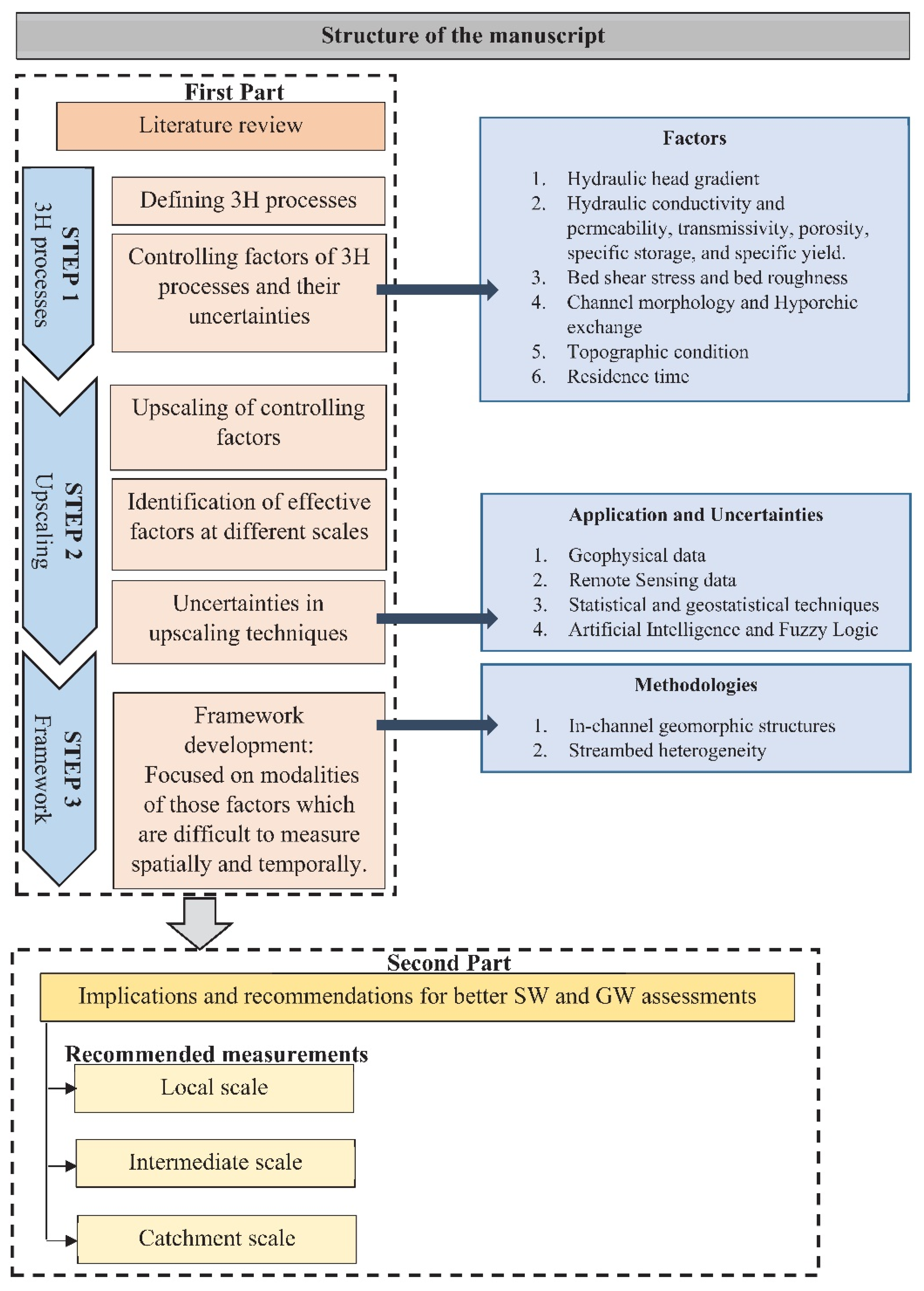
2. Literature Review

2.1. 3H Processes

Hydraulic processes in SW and GW systems are referred to as the movement of water volume and their associated pressure and energy. These processes depend on streambed pressure and water surface profile, which sequentially influences hydraulic head gradient and hyporheic exchange (HE) [23]. HE is primarily controlled by energy head gradients, alluvium volume, and hydraulic conductivity [24].

Hydrological processes in SW-GW interaction are referred to as in-channel pre-infiltrated water and their effect on changes in channel morphologies, transportation and deposition of sediments, development of in-channel geomorphic structures, and spanning of in-channel obstructions. The intensity of hydrological processes depends mainly on the spatio-temporal precipitation, heterogeneous topography, and floodplain anthropogenic activities.

Hydrogeological processes in SW-GW interactions can be divided into an HF and GW flow. The HF is bidirectional and travels a short distance, while GW flow is unidirectional and travels over much longer distances [7]. The HE due to hydrogeological processes mainly depends on streambed heterogeneity, subsurface geology, local topography, precipitation, and GW level position. Streambed heterogeneity depends on the bed composition, primarily controlled by channel slope and river sinuosity [25]. Bed composition includes alluvial beds composed of higher silt and clay, sandy bed, a mixture of both alluvial and sandy beds, unconsolidated materials, boulder bed, and bedrock with limited alluvial materials.

2.2. Controlling Factors of 3H Processes and Their Uncertainties

2.2.1. Hydraulic Head Gradient

Hydraulic head is the sum of pressure head, elevation head, and kinetic energy. It is used to characterize the mechanical energy of the fluid in SW and GW systems. At a point scale, hydrostatic components lead by the height and slope of SW cause the hydraulic head gradient changes. At a local or regional scale, the hydraulic head changes due to hydrodynamic components lead by stream velocity flowing over submerged bedforms, which results in momentum transfer to the bed [7]. Hydraulic head changes are also controlled by bed shear stress, bed roughness, and low and high-velocity zones in in-channel geomorphic structures such as spanning logs, pool-riffle, or riffle-pool sequences [7]. Controlling factors of hydraulic processes are shown in Figure 2.

The hydraulic head gradient in mountain streams is mainly controlled by in-channel obstructions, where high and low-pressure zones developed upstream and downstream of obstruction, which improves hyporheic circulation under the obstruction [24]. Uncertainties are associated with the identification of in-channel obstructions at a local to regional scale due to the distribution of in-channel geomorphology. Recent studies tried to identify in-channel geomorphic structures with different methodologies. Mahdade et al. [26] identified pool-riffle sequences at a spatial scale using wavelet and index methods, limited for low discharge rivers and large-scale undulation in the streambed. An increment in hydraulic resistance and SW-GW interaction due to the presence of in-channel logjams creates variations in the hydraulic head along the streambed. In this case, SW-GW interaction has been affected due to limited or generalized streambed leakage coefficient and hydrogeological properties. Spatial complexity has also increased along the streambed due to in-channel logjams. The reason for the spatial complexity is the presence of a control site both up and downstream. The upstream control site affects the downstream control site and hence impacts the results [27]. The spacing between individual geomorphic structures impacts the HE. For example, pool-step-riffle produced 60% downwelling and 40% upwelling, while riffle-pool-step reverses the percentages [28,29]. It showed the importance of accurate identification of in-channel geomorphic structures.

2.2.2. Hydrogeological Parameters (Hydraulic Conductivity, Permeability, Transmissivity, Porosity, Specific Storage, and Specific Yield)

Hydraulic conductivity is one of the leading factors in estimating and controlling HE flux across streambed spatially and temporally. Brunner et al. [3] and Naganna et al. [30] reviewed in detail several hydraulic conductivity measuring methods of in-situ, laboratory, and numerical modeling with some of their advantages and disadvantages. All techniques of determining hydraulic conductivity have uncertainties that are highly dependent upon the conditions under which the tests have been conducted [31]. Hydraulic conductivity of streambed is affected mainly by the heterogeneity of streambed, where its estimation is the most challenging task. The range of average error between measured and estimated hydraulic conductivity values with different methods and locations is of several orders of magnitude [3,31].

At point scale, field permeameter tests using the Darcy equation and the coupled seepage/hydraulic gradient method are not suitable techniques in estimating vertical hydraulic conductivity due to test design and logistics. However, the seepage meter is limited to a low-energy flowing stream and immobile bed [31]. Slug tests have generally been performed in wells (installed with filter packs) for water sampling. Uncertainty in the slug test is due to the borehole radius and the porosity of filter packs. Uncertainty in grain size distribution analysis leads to overestimation in hydraulic conductivity values precludes streambed anisotropy and is unable to consider preferential pathways [3]. Pumping tests have also been used for decades in hydraulic conductivity measurement. It also provides subsurface heterogeneity through the hydraulic tomography approach [3]. There are numerous challenges to overcome to conduct groundwater systems using a pumping test, such as coastal aquifer systems, fractured rock aquifer systems, shallow alluvial aquifer systems, determining aquifer properties, and well performance.

From the local to regional scale, statistical and geostatistical methods can be used to estimate heterogeneous hydraulic conductivity. However, these methods also have uncertainties and limitations as discussed by Naganna et al. [30]. For example, inaccuracies due to the density of in-situ point measurement in geostatistical technique [32]. The geostatistical methods usually do interpolation using the kriging method. The interpolated values at unknown locations depend upon the variance of in-situ point measurement. This variance shows the spatial dependency between the estimated points. If the nugget (related to short-range variability in the data) and sill (total variance where the empirical variogram appears to level off) ratio is <0.25, there will be a strong spatial dependency between the in-situ measured points [33]. With an increase in the nugget/sill (a component of the variogram), the error would increase in the estimated heterogeneous hydraulic conductivity. Uncertainties in other spatial measurement methods like geophysical and remote sensing have been discussed in the following sections.

Intrinsic permeability in alluvial beds increases with increasing particle size, while in an unconsolidated bed, it is affected by particle shape, particle packing, and degree of compaction [34]. Laboratory methods for the determination of permeability have some issues. First, it is less suitable for a mixture of silt and clay deposits [35]. Second, the packing and density of deposits are compromised during sample data collection. Third, if the sample is collected correctly, the core can provide only vertical permeability [34]. Chappell and Lancaster [36] studied the spatio-temporal uncertainties in the measurement of permeability in several field methods. MacDonald et al. [34] showed the importance of d10 cover in the variation of hydraulic conductivity in a catchment. Measurement of permeability and hydraulic conductivity values using repeated Guelph permeameter showed a good method in determining permeability, where large-scale permeability testing is not feasible.

Subsurface rock could be sedimentary or igneous, or metamorphic at or below the HZ. Permeability developed due to secondary porosity of rocks such as faults, joints, shear lineaments, facies, bedding plane partings, crossbedding, dipping beds, axial plane cleavage, and other fractures [30]. Hydraulic conductivity values vary vertically and laterally following the direction of the above-mentioned secondary porosities. Bi-directional flow in fractures and the bedding system recharges the aquifer, at a local or regional scale, either from downward seepage or lateral/upward seepage. Water flow through subsurface geological settings is controlled by aquifer characteristics (transmissivity, storativity, specific storage, and specific yield), compressibility, and effective stress of the aquifer. The movement of water is either SW to GW or within the aquifer. The magnitude of the SW-GW interaction in the groundwater system depends upon the effective porosity (specific yield; Sy) of the crystalline rock aquifers. Dewandel et al. [37] proposed an upscaling method based on the double water table fluctuation for the estimation of hydraulic conductivity and Sy. This information is useful as input parameters for the GW numerical modeling. However, this proposed method required a significant amount of borehole information that discourages in cases of limited information and shows the inability to estimate spatial heterogeneity.

2.2.3. Bed Shear Stress and Bed Roughness

Bed shear stress is mainly controlled by bed roughness such as stream metabolism, drag coefficient, and velocity generated due to the dynamic pressure [38]. Bed roughness varies according to hydraulics, geomorphology, and sediment condition in a river. Uncertainties in streambed mobilization are due to the generalization of roughness factors, visual identification of sediment texture, and several discharge-related conditions [38]. The presence of roughness factors such as streambed vegetation and gravel bed (generally in mountain streams) affect flow velocities, shear stress, and turbulence intensities. For example, streambed anisotropy enhanced by vegetation generates strong secondary currents and develops a new boundary layer by changing bed roughness from gravel bed to vegetated bed [39]. Ignoring these factors or imprecise estimation/identification of roughness factors develop uncertainties in hydraulic processes. The drag coefficient varies due to blockages in a river either by in-channel obstruction or geomorphic structures, the flow area of a cross-section, local velocity, and local water depth. At a local scale, an increment in bed roughness, due to in-channel obstruction can modify the transportation and deposition of sediment [40]. Modification of channel morphology causes changes in flow velocity, and momentum affects dynamic pressure head distribution [24]. Therefore, in the drag coefficient estimation, the ignorance of in-channel obstruction causes uncertainties in hydraulic processes. For example, Hygelund and Manga [41] investigate the effect of wood logs on the drag coefficient with the orientation, size, depth, and leafless log branches.

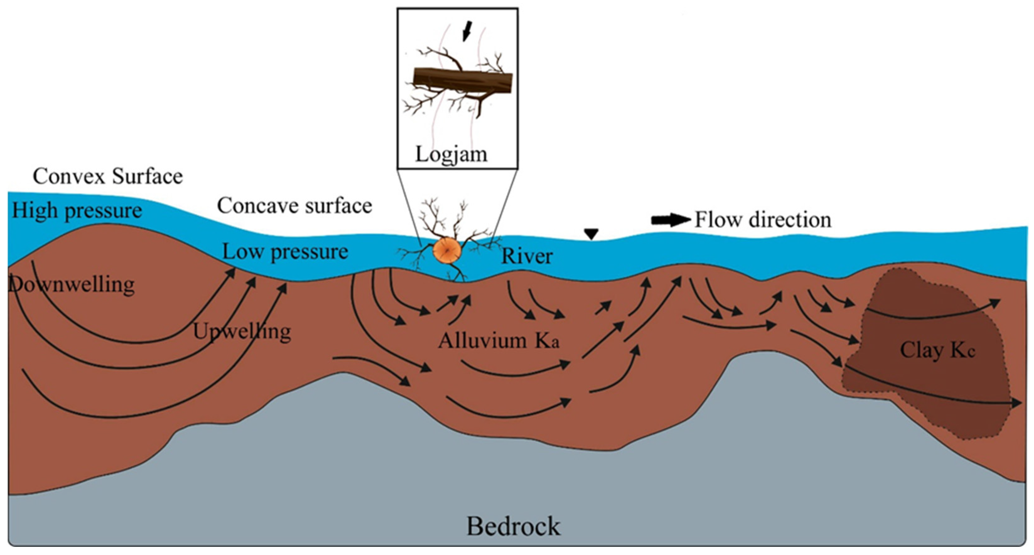
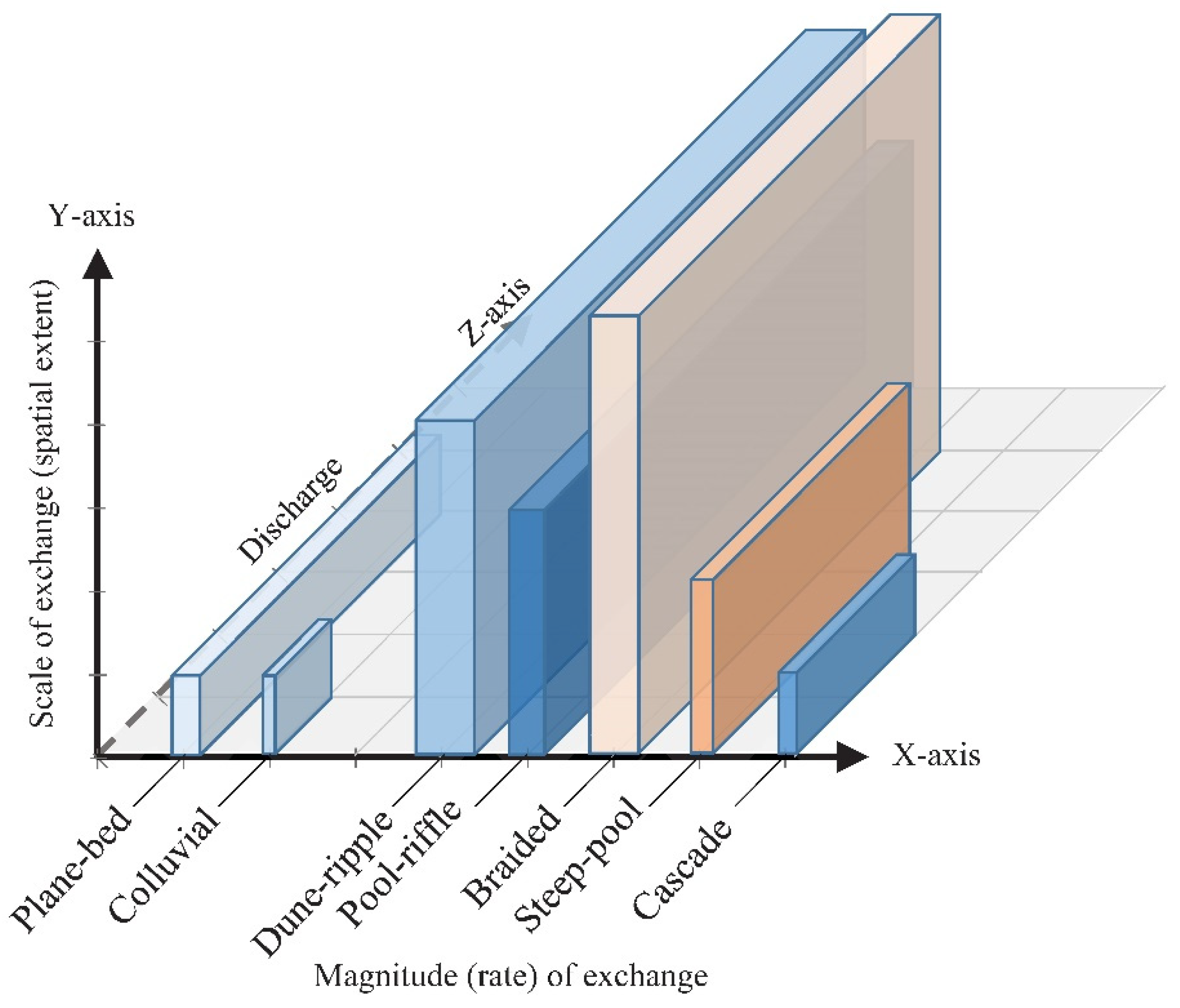
2.2.4. Channel Morphology and Hyporehic Exchange

Three factors have controlled the modification in channel morphology [42]. First, the effect of soil and climatic conditions on the discharge regime; second, variation in channel slope according to heterogeneous topography from local to regional scale; third, the impact of sediment properties on streambed erodibility. All these factors in different types of channels were discussed in detail by Montgomery and Buffington [43]. Further discussion is not required because the focus is on the rate and spatial extent of HE. Buffington and Tonina [25] showed different relationships between magnitude, spatial extent, the length scale of HE, and river discharge. In this review, these relationships are combined to show the heterogeneity of hydrological control on HE in different channel types (Figure 3).

Schmadel et al. [44] analyzed the spatial heterogeneity of hydrological control on HE in steep-pool morphology. They found that GW inflow was the primary controlling factor rather than discharge in morphologically driven HE. Whereas, spanning of a channel structure such as natural debris dams, stream restoration log dams, and boulder weirs cause dominancy of hydrostatically derived HE and reduction in hydrodynamic forces [45]. The significance of hydrological processes is limited to examining variation in channel morphology and its effect on HE. Mostly, uncertainties of hydrological processes in SW-GW interactions are due to hydrological modeling that has been discussed in the later section.

2.2.5. Topographic Condition

The relationship between topographic conditions and GW level position is responsible for controlling GW flow, infiltration, and exfiltration in the HZ. Sophocleous [46] mentioned the extension of GW discharge from the discharge area to the downgradient from the basin hinge line (an imaginary line separating discharging and recharging areas). Dahl et al. [4] classified riparian flow paths based on the type of flow and contact time between water and riparian deposits with an organic content as diffused, overland, direct, and drainage flow path. The mechanism of these flow paths is helpful in understanding the recharging and discharging of GW, mainly derived by precipitation. The extent of the HZ due to these flow paths varied spatially and temporally. For instance, during the GW upwelling, the HZ depth is constant across the stream’s width due to a diffused flow path than the direct flow path. Whereas, during the GW downwelling, the HE occurs in shallow sediments of the stream’s central part [47].

2.2.6. Residence Time

Another effect of flow paths (mentioned above) is on residence time, controlled by the flow path scale and hydraulic conductivity heterogeneity. High residence time (from weeks to years) is associated with a diffused flow path, while short residence time (for a few hours) is associated with a drainage flow path [4]. Heterogeneous hydraulic conductivity increases the tortuosity of flow lines causing uncertainty in measured residence time. Whereas, in the homogeneous case, the increment in residence time is due to the compression of the HZ. The overall effect of heterogeneity and homogeneity of residence time is due to variation in the HZ and HE, which influence reactive transportation [48]. Additionally, the HZ extent in a floodplain is controlled by lateral flow paths that follow paleo-channels across a floodplain or the head difference between meanders in the stream path [49]. Meander-driven lateral flows are the greatest from hinge points, controlled by channel sinuosity and settings with large GW discharge rates [49].

Summary of controlling factors of 3H processes and their uncertainties are given in

Table 2. Summary of 3H processes controlling factors, their sub-factors, and uncertainties.

Processes	Controlling Factors	Scale	Sub-Factors	Uncertainties
Hydraulic	Hydraulic head gradient	Point	Affected by height and slope of SW	Coarse-resolution and inaccurate measurement of SW height.
		Local or regional	Affected by bed roughness, stream velocity, and bed topography	Use of constant bed roughness and streambed leakage coefficient. Ignorance of geomorphic structures.
Hydrogeological	Hydraulic conductivity	Point	Affected by streambed heterogeneity	Inaccurate grain size distribution
		Local or regional	Affected by streambed heterogeneity and secondary porosity	Low-density point measurement and ignorance of secondary porosities.
	Permeability	Point, local or regional	Particle size, shape, packing, and degree of compaction	Lab-based measurements
Hydrological	Bed roughness	Local or regional	Streambed vegetation, gravel bed, and channel morphology	Selection of wrong bed roughness or ignorance of bed roughness factors.
	Drag Coefficient	Local or regional	In-channel obstruction or geomorphic structures, and river geometry.	Ignorance of in-channel obstruction
	Channel morphology	Local or regional	Soil and climatic condition, heterogeneous topography, and sediment properties	Ignorance of key factors and hydrological modeling limitations.

.

2.3. Upscaling and Role of Effective Factors at Different Scales

In SW-GW interactions, scales vary from point to regional and their selection depends on the type of study. For example, water quality assessment due to anthropogenic activities is generally studied at specific locations, while water resource management is at a regional scale/watershed scale. Mostly in-situ measurements are at point scales, which can interpolate to a larger scale for precise assessment of SW-GW interactions. The importance of upscaling is explained by Boano et al. [7] while dominating characteristics and factors of different scales are briefly discussed by Barthel and Banzhaf [5]. Effective factors in SW-GW interactions are variable at different scales. How the effective factors change from one scale to another scale, and how they can interpolate during the transition is not addressed correctly in the literature. It needs to be comprehensively classified to understand upscaling and downscaling between different scales. Furthermore, the role of integrated techniques needs to assess in the above scenarios.

2.3.1. Effective Factors at Different Scales

At the point scale, very detailed observations are possible in describing elementary and fundamental concepts of 3H processes [5]. Upscaling of the elementary and fundamental concepts is challenging due to (i) heterogeneity and complexity, which gives inaccurate results when low-density point scale measurements are interpolated and (ii) restriction in high-density point measurements on the field due to high cost, high labor, and impractically high measurement times. As discussed, in upscaling, some factors become less important with increment in the heterogeneity and complexity from point scale to a larger scale, whereas the importance of other factors becomes more relevant than at the point scale. However, the influence of insignificant factors at a point scale continues to exist at a larger scale but lies outside the area of interest. For example, at the point scale, SW-GW interaction is due to changes in pressure gradient between GW and SW bodies affected by pore geometry, size, distribution, and connectivity of streambed with an aquifer [5]. While at a larger scale, the effects of pressure gradient are studied in terms of exchange flux between in-channel geomorphic structures, unsaturated zones, hydrostatic and hydrodynamic processes.

Several authors have mentioned different criteria for the relevancy and irrelevancy of processes and parameters at different scales which are summarized by Barthel and Banzhaf [5]. In this study, the relevancy and irrelevancy of all possible processes and parameters were identified based on different criteria. The criterion to simplify the descriptive comparison of the effective parameters from small to large scale are summarized as follows:

• Processes and their parameters in HZ can be observed in detail at a small scale, while these have strong practical limits at a larger scale. However, nature and magnitude are unchanged at a larger scale. Therefore, parameters are irrelevant at a larger scale and relevant at a smaller scale for study purposes.
• There are some processes and parameters which give detailed observation at a small scale but can only be observed at a large scale. Therefore, for study purposes, large-scale assessment of those processes and parameters is the only option.
• However, for some parameters at larger-scale studies, observations at low resolution will suffice. Therefore, some detailed observations at a small scale become irrelevant.

Based on the criterion obtained from the literature, variations of effective factors at different scales are shown in

Table 3. Relevancy of effective factors at different spatial scale.

Processes	Factors	Sub-Factors	Point	Local	Intermediate	Regional
Hyd	1	Pressure gradients	R	R	IR	IR
Hyd	1	Hyporheic flow	R	R	PR	IR
Hyd, Hyg	1, 2	Streambed leakage coefficient	R	PR	IR	IR
Hyd	1	Turbulence intensities	IR	R	IR	IR
Hyd, Hy	1, 3	Stream velocity	IR	R	PR	IR
Hyd, Hy	1, 3, 4	Stream’s water surface slope	IR	PR	R	R
Hyd, Hyg	1, 2	Geomorphic structure, its size and spacing	IR	PR	R	R
Hyd	1	Channel obstructions	IR	PR	R	R
Hyg	2	Pore size and distribution	R	IR	IR	IR
Hyg	2	Pore geometry	R	IR	IR	IR
Hyg	2	Streambed porosity	R	R	IR	IR
Hyg	2	Connectivity of the aquifer substratum and riverbed	R	R	PR	IR
Hyg	2	Hydraulic conductivity	R	R	IR	IR
Hyg	2	Permeability	R	R	IR	IR
Hyg	2	Transmissivity	R	R	IR	IR
Hyg	2	Streambed composition	R	R	IR	IR
Hyg	2	Infiltration rate	R	R	IR	IR
Hyg	2	Thickness of sediment layers	R	R	IR	IR
Hyg	2	Grain size distribution	R	R	IR	IR
Hyg	2	Groundwater level	R	R	R	R
Hyg	2	Intrinsic permeability	R	R	IR	IR
Hyg	2	Biological activities	R	R	IR	IR
Hyg	2	Groundwater chemistry	R	R	PR	IR
Hyg	2	Groundwater discharge rate	IR	PR	R	R
Hyg	2	Clogging layer of streambed	IR	IR	R	IR
Hyg	2	Groundwater flow	IR	IR	R	R
Hyg	2	Aquifer characteristics	IR	IR	R	R
Hyg	2	Aquifer compressibility	IR	IR	R	R
Hyg	2	Parent-rock type	IR	IR	R	R
Hy	3, 4	Depth to bedrock	R	R	IR	IR
Hy	3	Streambed motion	IR	R	IR	IR
Hyd, Hy	1, 3	Bed shear stress	IR	R	IR	IR
Hy	3	Streambed vegetation	IR	R	PR	IR
Hy	3	Roughness features	IR	R	R	R
Hy	3, 4, 6	Channel slope	IR	PR	R	R
Hy	3, 4	Drag coefficient	IR	PR	R	R
Hy	4	Channel morphologies	IR	PR	R	R
Hy	4, 5	Precipitation	IR	PR	R	R
Hy	5	Surface topography	IR	PR	R	R
Hy	5	Floodplain anthropogenic activities	IR	PR	R	R
Hy	5	Evaporation	IR	IR	IR	IR
Hy	5	Soil heterogeneity	PR	PR	PR	PR
Hy	5	Climate	R	R	R	R
Hy	5	Geological structures	IR	IR	IR	IR
Hy	6	Residence time	IR	IR	IR	IR
Hy	5	Evapotranspiration	R	R	R	R
Hy	1, 4	Environmental tracers	R	R	R	R
Hy	4	Water chemical characteristics	IR	IR	IR	IR
Hy	4	Channel geometry	IR	IR	IR	IR
Hy	4	Bank storage	R	R	R	R
Hy	5	Soil moisture	R	R	R	R
Hy	3, 4	Hydraulic structures	IR	IR	IR	IR
Hyg, Hy	2, 4	Pumping	IR	IR	IR	IR
Hy	4	River network	R	R	R	R
Hy	5	Land use changes	R	R	R	R

R is relevance, IR is irrelevance, PR is partially relevant, Hyd = hydraulic, Hyg = hydrogeology, Hy = hydrology, Factor 1 = Hydraulic head gradient, Factor 2 = hydrogeological parameters, Factor 3 = Bed share stress and bed roughness, Factor 4 = Channel morphology and Hyporehic exchange, Factor 5 = Topographic condition, and Factor 6 = Residence time.

.

The table summarizes that the effectiveness of factors changes from a small scale to a larger size [5]. For example, at a point and local scale, channel slope is ineffective while it is effective at a larger scale due to lateral variations in streambed elevations. The streambed leakage coefficient is effective at point scale while it is less effective at a larger scale due to heterogeneous streambed composition and changes in streambed thickness, where the spatial determination of the coefficient is not possible. The role of geomorphological structures and channel obstruction in SW-GW interactions is effective at a larger scale, while these are ineffective at a point and local scale due to their heterogeneous spatial extent and processes responsible for their formations. However, these structures are responsible for increasing intensities of HE at a point and local scale, which indicates relationships between effective and ineffective factors at different scales. Although, factors at a larger scale can be determined by inverse modeling with other factors that required some form of generalization and hence create uncertainties in effective GW resource management.

2.3.2. Integration of Effective Factors during Upscaling

For accurate integration of effective factors, a large number of in-situ data is required. It could be from high-density point measurements, which is impractical as discussed above. It could be from a large number of borehole data in the study area, which provides detailed vertical information and can interpolate spatially. However, the availability of high-density borehole data is also rare. It could also be from environmental tracers that provide an average measurement but are unable to characterize spatial heterogeneity. Alternatively, geophysical methods can be used to identify SW-GW interactions at both vertical (centimeters to hundreds of meters) and horizontal scales (meters to hundreds of meters). Remote sensing provides a synoptic view of large areas, coupled with geophysics and geographic information system plays a crucial role in enhancing the characterization of SW-GW interactions.

2.3.3. Uncertainties in Geophysical Data for Characterization of SW-GW Interactions

McLachlan et al. [50] reviewed geophysical methods that provide geological, hydrological, and biogeochemical information spatially and temporally. McLachlan et al. [50] mentioned three primary uncertainties of the geophysical approach. First is the uncertainty in geophysical data and modeling methods. Several under and overestimation measurements caused a misinterpretation of subsurface information. The accuracy of subsurface information is affected due to errors in a model structure like the limitation of software and algorithms of image processing and interpolation. Various approaches to solve and formulate inversion problems for the interpretation of subsurface geology are reviewed by Linde et al. [51]. Second is the resolution of geophysical data, which is affected due to the number and spacing of electrodes. A large number and small spacing of electrodes are used to obtained detailed subsurface information, whereas a lesser number and wide spacing of electrodes are used to obtain deep but also some generalized subsurface information. The third is the extraction of quantitative information from geophysical and petro-physical data, which is inconsistent due to different resolutions.

Improvement in these uncertainties can be a good calibration of geophysical data with other in-situ data such as solute transport, point scale measurements, and borehole data. Multiple geophysical methods such as coupling of resistivity and seismic data with anomalies obtained from magnetic and gravity surveys are also useful for the improvement. Moreover, the selection of the best methods based on the objectives of a study is crucial. It requires the proper arrangement of an instrument such as straight and well-spread lines, adequate current input, strong input signals, no external noise, and many more [52]. Furthermore, the fence diagram of geophysical data used for validation where the crossing point of 2D subsurface images must be of the same values [53].

Improved geophysical data will play an important role in the characterization of SW-GW interaction. Randomly collected geophysical data such as streambed heterogeneity, subsurface porosity, geomorphic structures, and subsurface aquifer characteristics can be interpolated for sub-catchment and catchment scale assessments. These data will also be helpful during the training of machine learning processes.

2.3.4. Use of Remote Sensing and Their Uncertainties for Characterization of SW-GW Interactions

The extraction of river bathymetry is one of the most challenging tasks during field surveys, especially at wide rivers. Accurate spatial measurement of river bathymetry is necessary, which leads to a variety of hyporheic processes (as discussed above). Remote sensing data is crucial for the spatio-temporal estimation of river bathymetry, changes in river morphologies, identification of geomorphological features, evapotranspiration, land-use changes, and extent of wetlands. High resolution (≤2.5 m) LiDAR-based Digital Elevation Models (DEM) are useful for accurate floodplain topography and river geometry [54,55]. Further limitations of DEM and the use of other satellite images for in-depth estimation were reviewed by Brunner et al. [3]. Several approaches have been developed for submerged topography of a river, based on the spectral reflectance of satellite images [56,57]. However, these still need to be improved. Remote sensing data coupled with geophysical data is constructive for better spatial estimation of rainfall recharge, GW table, GW volumes, fluxes, and flows from a local scale to a regional scale [58].

Thermal infrared imaging (TIR) remote sensing is another technique for mapping temperature patterns and thermal anomalies in water bodies. Diurnal and annual variations in SW temperature and relatively stable GW temperature were used to identify hydraulic connections between aquifers and rivers. Additionally, it is useful in mapping spatial surface temperature patterns along rivers from a local to regional scale. Generally, hydro-geochemical (stable isotopes) data coupled with the TIR is used to validate the TIR-based SW-GW interaction [59,60,61].

Uncertainties in remote sensing data are primarily due to satellite image resolution, cloud cover, spectral characteristics, and noises. Publicly available remote sensing data have a coarse resolution (15 m), which can be used to estimate evapotranspiration. Fine resolution (≤2.5 m) is constructive to obtain other surface information precisely. In the cloud cover case, the use of multiple images of different temporal resolutions of that particular area is useful. Uncertainty due to spectral characteristics causes misinterpretation of different objects. It can be improved by coupling with either field survey data or information from higher resolution images [62]. Spatio-temporal surface temperature patterns, from local to sub-catchment scale, are mapped with low altimeter TIR mounted on Unmanned Aerial Vehicle (UAV). For accurate characterization of SW-GW interaction at a catchment scale, it provides precise spatio-temporal surface temperature patterns.

2.3.5. Uncertainties in Statistical and Geostatistical Techniques for Interpolation of Effective Factors

The application of statistical and geostatistical techniques is used to generate spatio-temporal maps and predictions of effective factors at unknown locations. Generally, interpolation required point measurements, which effects due to low-density point measurements and model structure. The 2D and 3D subsurface measurements using hydro-geophysics and remote sensing are useful for improving the interpolation accuracies. For example, the relationship between precipitation, runoff, and infiltration rate is necessary to understand accurate water balance. The relationship is affected primarily by the spatio-temporal measurements of precipitation due to low-density gauge stations. This uncertainty is addressed in the literature using pixel-based spatio-temporal estimation coupled with geostatistical techniques and factors affecting precipitation [63,64,65]. Additionally, 2D and 3D geophysical data are interpolated using several interpolation methods such as model-driven or based on wave-equation, and data-driven or based on signal processing [66]. However, for precise interpolation, these methods are coupled with a local variogram, which represents local structural anisotropies [66]. Naganna et al. [30] reviewed several statistical and geostatistical models with their application and implications. Furthermore, geophysical data coupled with TIR and hydro-geochemical data could provide accurate SW-GW interaction maps at a catchment scale.

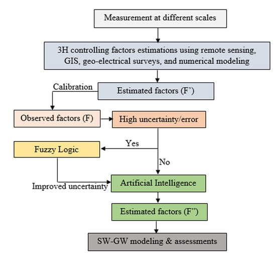
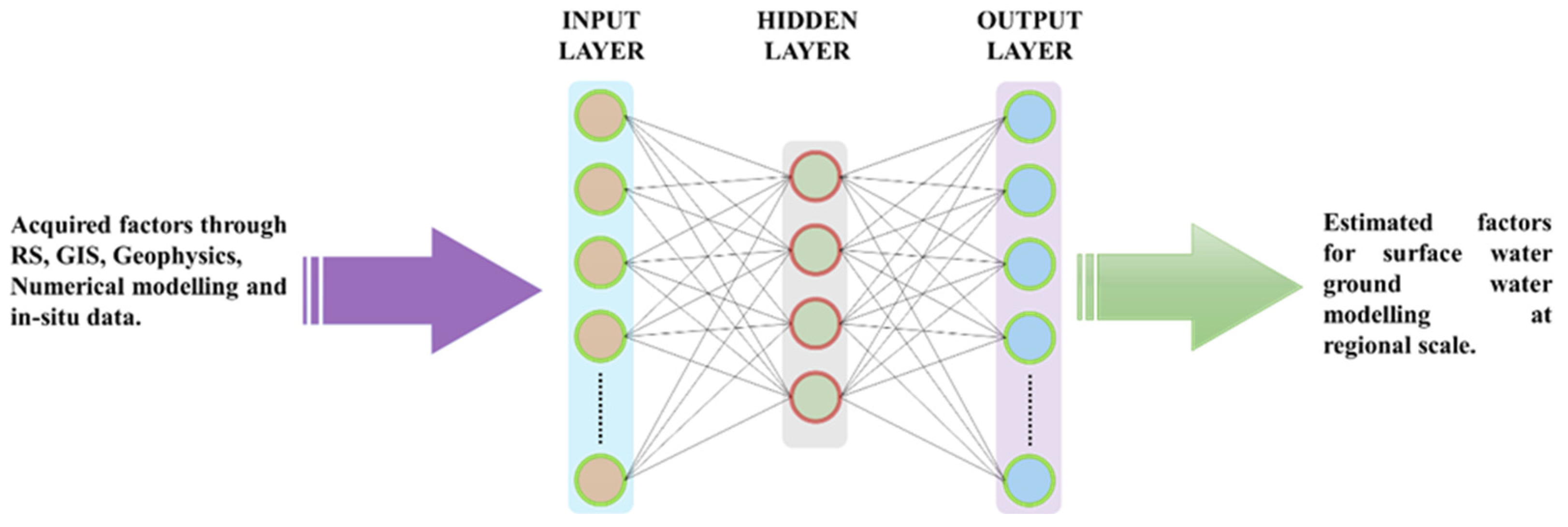
2.3.6. Use of Artificial Intelligence and Fuzzy Logic for Characterization of SW-GW Interactions

Artificial Neural Network (ANN), inspired by biological neural networks, proves to be a powerful tool that can be structured to perform multiple complex tasks like classification, forecasting, pattern recognition, and process modeling. The ANN is an effective tool in inferring a factor via other factors without any specific relationship. An ANN requires training by searching an optimal value of biases and weights to obtain an accurate relation between input and output. This training process minimizes the error between the estimated and the observed output values step by step.

As shown in Figure 4, using ANN, the SW-GW interaction can estimate at a regional scale, where the effecting factors at a point or local scale are used to train the ANN, and estimate the factors corresponding to the regional scale. This estimation can be done using an optimally structured ANN employing one hidden layer and inputs corresponding to the number of affecting factors incorporated in the study.

The ANN posed with more training data, allows the process to converge the network towards more accurate values. A major concern during the training is network over-fitting, which can be avoided by dividing the data into three sets such as training, validation, and test.

Chang et al. [67] investigated SW-GW interaction by correlating GW level variation, rainfall, and streamflow using the ANN approach. Rajaee et al. [68] reviewed AI methods in GW level modeling in which they explained the widely used AI methods and their modalities and algorithms [69,70,71,72,73]. They mentioned uncertainties of AI methods such as overtraining, low generalizability, risk of using unrelated data, and incorrect modeling. Almost all previous studies used ANN in GW level estimation and water quality modeling. A few studies used ANN in the characterization of SW-GW interactions. Spatio-temporal data collection for GW level and water quality modeling is challenging due to limited boreholes from where data are easily collected. Accurate SW-GW interaction modeling using ANNs can be possible with big data obtained from geophysical and remote sensing techniques. A discussion on the possible modalities of SW-GW interaction is in the following sections.

The fuzzy logic approach is like a human decision-making methodology, which deals with uncertainties due to vagueness in input data, factors, and model structure. It works by solving possibility theory using fuzzy numbers instead of crisp numbers to minimize uncertainties and complexities of hydrological models [74,75]. There are several fuzzy logic operations such as fuzzification, fuzzy logic operators, fuzzy inference system (FIS), and defuzzification based on appropriate membership functions (MFs) from the specified input-output pairs. Multiple techniques coupled with combined ANN and FIS in GW level modeling with Mamdani and Sugeno approaches have been used [68,76]. Milan et al. [77] used FIS in SW and GW resource management to reduce GW modeling uncertainties using MODFLOW. Other studies used fuzzy logic coupled with remote sensing and GIS for potential GW mapping [78,79]. None of the studies used a fuzzy approach to reduce uncertainties in SW-GW interaction modeling. It would be an accurate approach in upscaling SW-GW interactions.

2.4. Framework Development

Based on the above discussion of the 3H processes, this section focused on modalities of those factors which are difficult to measure spatially and temporally. These factors are geomorphic structures and streambed heterogeneity in hydraulic processes; channel morphology, which includes sediment deposition and floodplain HZ in hydrological processes; subsurface geology, streambed composition, secondary porosity, and aquifer characteristics in hydrogeological processes. Some factors are not discussed in detail because their methodologies are common. For instance, channel morphology can be easily identified by visual interpretation techniques using remote sensing data. Spatio-temporal sediment deposition can be estimated through hydrological modeling using in-situ sediment grain size distribution data. Floodplain HZ can be identified by mapping temperature patterns and thermal anomalies in water bodies using TIR remote sensing technique (as discussed in Section 2.3.4). Furthermore, subsurface geology, secondary porosity, and aquifer characteristics are generally measured using geophysical surveys.

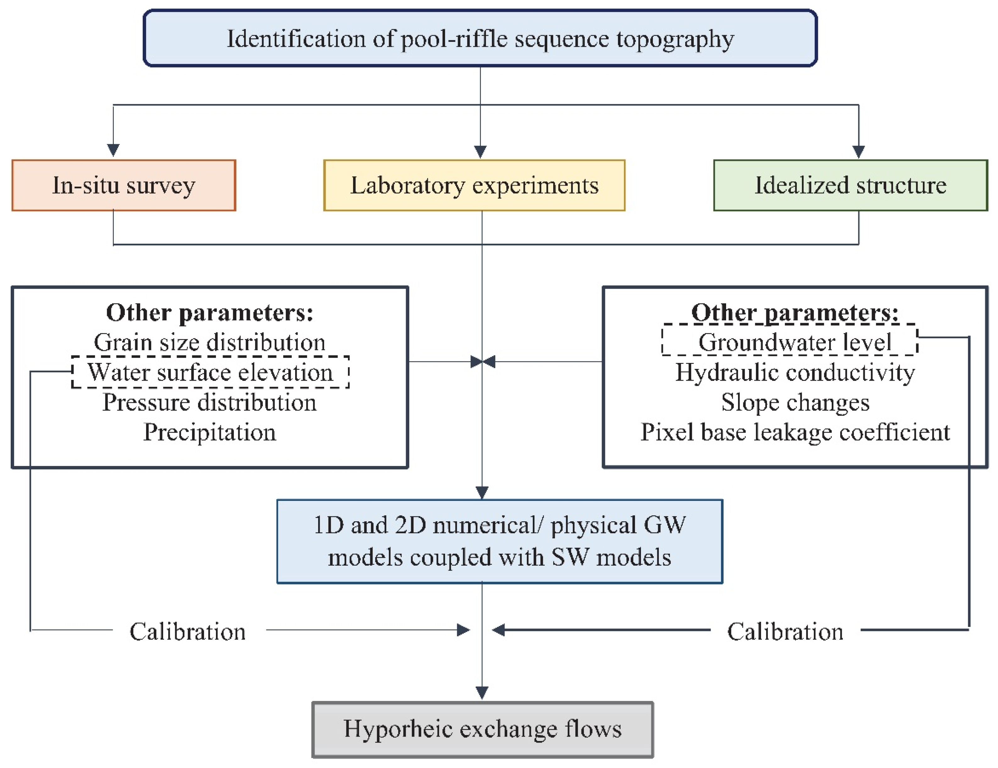
2.4.1. Identification of In-Channel Geomorphic Structures

The mapping of log jams in a natural channel is studied by Doughty et al. [27], while others used artificial logjams in laboratory experiments. Doughty et al. [27] analyzed HE flow variation due to log jams at a local scale using tracer injection, electrical resistivity imaging, numerical modeling, and statistical methods. The general approach is the data collected from tracer injection and electrical resistivity is used in numerical modeling to simulate HE flow and solute transport (Figure 5).

Small-scale HE flows, both vertically and laterally, are derived by changes in longitudinal gradients due to the presence of pool-riffle and steep-pool sequences. At a local to regional scale, visible in-channel geomorphic structures in shallow water can be identified using high-resolution satellite images and aerial photographs [56,57]. For geomorphic structures in deep water, geophysical surveys or sound navigation ranging (SONAR) could be useful. Mostly, previous studies identified pool-riffle sequences from in-situ data, while some used idealized pool-riffle structure and laboratory-based pool-riffle topography [28,80,81,82,83,84]. The combined methodology of these studies to analyze HE flows are shown in Figure 6.

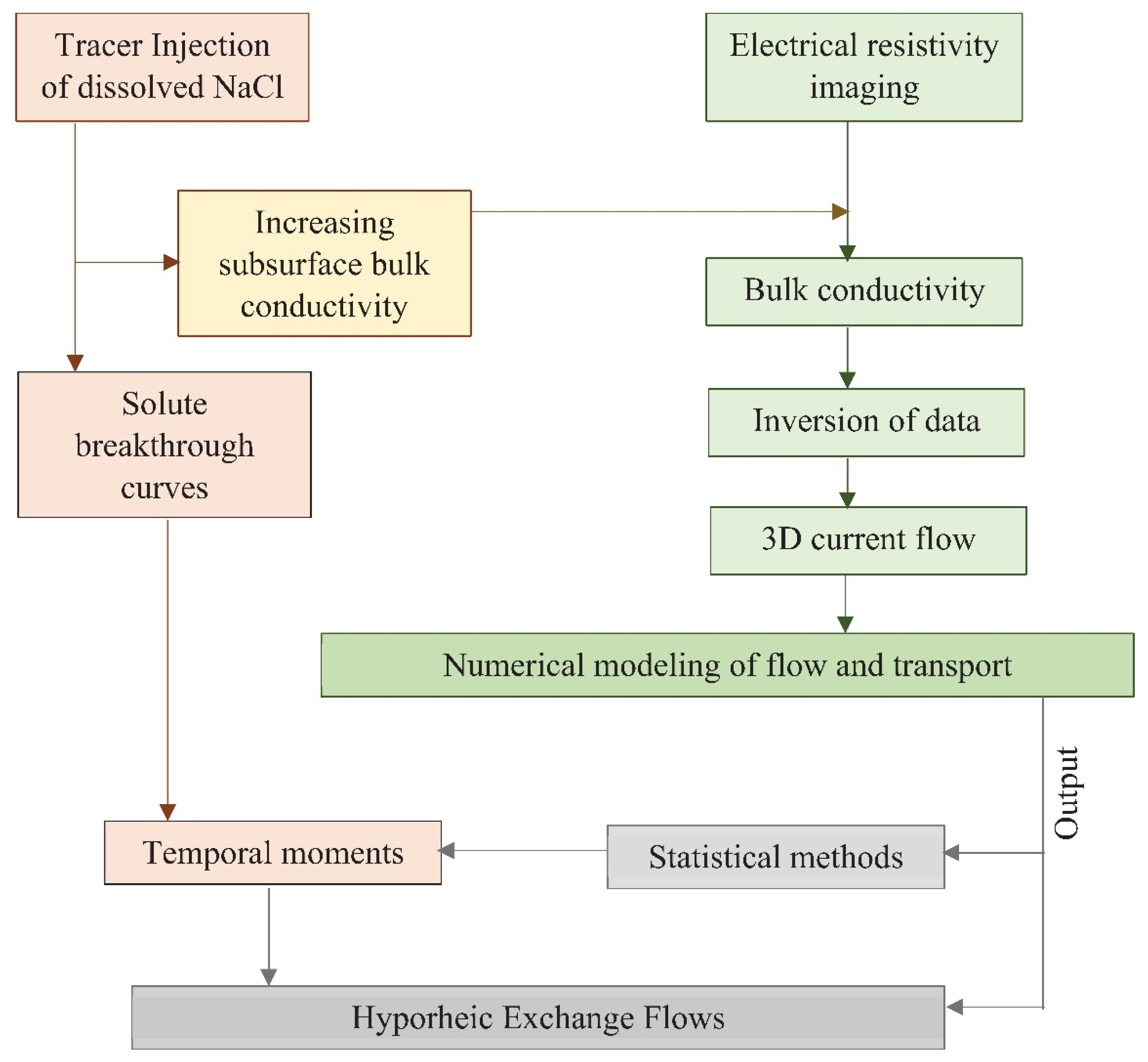
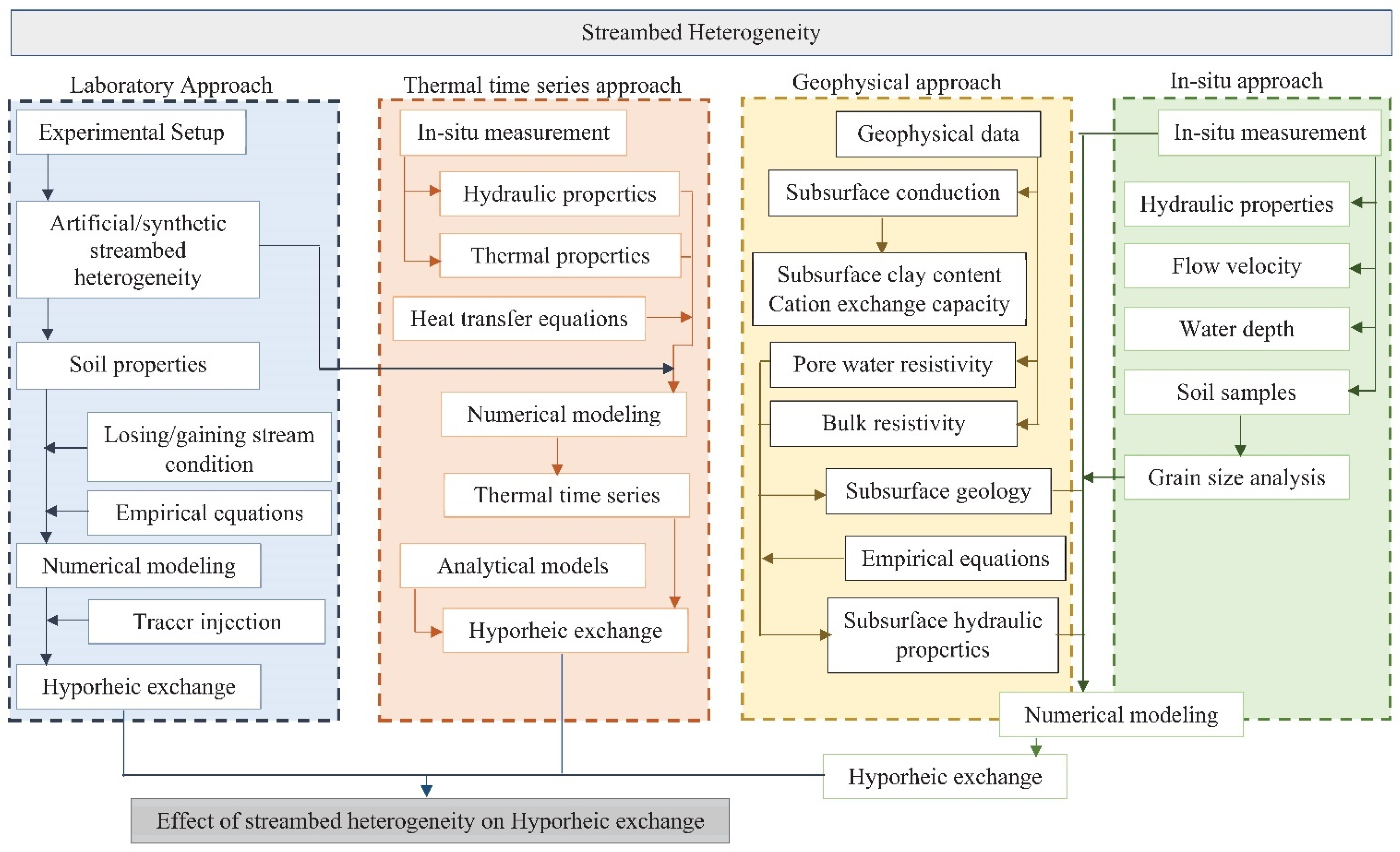
2.4.2. Measurement of Streambed Heterogeneity

Measurement of streambed heterogeneity is a challenging task because it is affected by channel morphology and topographic factors. For instance, in the meandering river, streambed features are more variable than a straight channel. Increases the streambed thickness due to the deposition of sediments with increasing river sinuosity. While in the straight channel, the thickness varies due to changes in channel slope and sedimentation rate. Several studies analyzed the effect of streambed heterogeneity on a HE through four types of approaches at a local scale. First is the laboratory-based, in which an experimental setup of the streambed with the composition of different materials [24,85]. The second is using spatial in-situ data, in which the data is either collected at river cross-section or random sampling [86].

The third is using thermal time series data, in which temperature sensors have been installed for data collection, interpolated through geostatistical methods, and modeled using empirical equations and numerical modeling [87,88]. Fourth is using geophysical methods, either across the river or along the river, depending on the water depth [89,90]. The combined methodology of these studies and their effect on HE flows are shown in Figure 7.

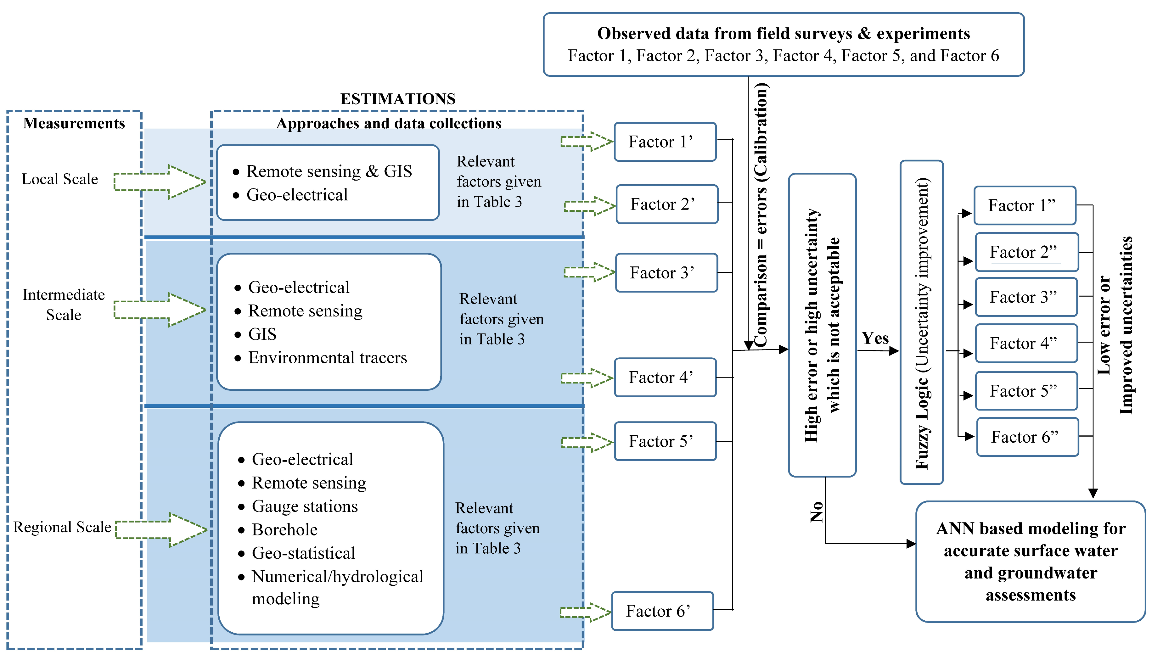
3. Proposed Framework

The framework is proposed based on this review. The purposes of the framework are accurate upscaling of 3H processes and big data assessment. Effective factors and uncertainties have been discussed in the above sections. Figure 8 shows the general layout of the proposed framework. Brief explanations of the proposed framework are as follows:

3.1. Local Scale Measurement

The local scale is referred to as a river cross-section with floodplain and adjacent geologic units [5]. Along the cross-section, three types of measurements are proposed.

First is point scale measurement covering the center of the river and left and right side from the center, including riverbanks [86]. Point scale measurement is mainly for calibration and validation purposes. The second is remote sensing data for bathymetry estimation and river-aquifer interaction. The third is geo-electrical methods such as electrical resistivity tomography (ERT), induced polarization (IP), and transient electromagnetic (TEM). Geo-electrical methods can accurately map streambed heterogeneity across as well as along the flowing river, which is one of the most important factors in SW-GW modeling [91,92]. Along the river, log jams may alter the measurement. In that case, across the river measurement at close intervals would be useful. Additionally, spatio-temporal mapping with geo-electrical methods is possible, which helps upscale streambed heterogeneity, rather than assuming homogenous streambed, as done by previous studies mentioned above. Furthermore, an in-channel geomorphic structure can accurately map with geo-electrical methods, which is crucial in hyporheic exchanges.

3.2. Intermediate Scale Measurement

The drainage area connected by several streams and tributaries is an intermediate scale [5]. At this scale, point scale and geo-electrical measurements covering all streams and tributaries are practically not possible. Therefore, geo-electrical surveys, remote sensing, and GIS are suitable for measuring variable channel morphology, and topographic characteristics. For example, low-density geophysical profiles are for a straight channel, while high-density profiles are for a meandering river. A high resolution (≤2.5 m) LiDAR-based digital elevation model (DEM) can capture accurate topographic characteristics of floodplain and dry parts of the river (means up to river water surface level). Limited in-situ water depth measurement can estimate the submerged river topography [56,57,93,94]. Additionally, spatio-temporal anthropogenic activities and land use land cover changes can accurately be determined using satellite images. Overall, for selected places using remote sensing, geo-electrical surveys can provide accurate floodplain soil heterogeneity, hydraulic properties of soil, and aquifer characteristics. Furthermore, the role of environmental tracers is crucial in understanding the spatio-temporal SW and GW quality, and pollution assessment.

3.3. Regional Scale Measurement

The regional scale in the proposed framework refers to the whole catchment. At this scale, the complexity is very high due to combined spatio-temporal variations of climate, geomorphology, geology, landscape types, and biological factors [5]. Upscaling at a regional scale is a tough and challenging task because of the size and heterogeneity of the catchment. In data collection at this scale, remote sensing, in-situ gauge stations, and borehole data played a primary role. Geoelectrical measurements are only practically possible and useful at prioritized areas at the regional scale, which depends on the objective of a particular study. However, the prioritization criteria depend on the types of analysis and investigations [95,96]. Extensively, inverse modeling is used to estimate hydraulic, hydrogeologic, and hydrologic factors for physical or numerical modeling of SW and GW. In inverse modeling, GW level data from a borehole and in-situ gauge stations of precipitation, river water level, discharge, and evaporation are crucial for calibration and validation purposes. Based on the topography, suitable statistical and geostatistical techniques would be accurate for the interpolation of scattered in-situ data. Overall, upscaling of 3H processes at a regional scale using multiple approaches with precise calibration and validation can provide an accurate assessment of SW-GW interactions.

4. Conclusions

This review presents the hydraulic, hydrological, and hydrogeological process (3H) and its controlling factors in the quantification of SW-GW interaction separately at local to regional scale, which has brought all aspects in one place. Additionally, the limitations, uncertainties, and challenges in controlling factors measurement of 3H processes at different scales are also discussed. The upscaling methods of effective factors and their associated uncertainties in 3H processes at different scales are not well understood. As well, the modalities for the characterization of SW-GW interaction at different scales are also missing in the available literature.

Based on peer-reviewed journal literature, the effective factors of 3H processes in the characterization of SW-GW interaction from local to regional scale are identified and emphasized on their upscaling and associated uncertainties. Upscaling techniques mentioned in the literature are lacking on how the effective factors from a local scale to regional scale could be accurately estimated. The role of electrical geophysics methods and remote sensing techniques in upscaling could be crucial, but presently, these are limited in use. The role of fuzzy logic in uncertainty improvement and artificial intelligence, especially artificial neural networks in analyzing big data, are widely applicable but very sparse in SW-GW interaction-related studies. Big data is crucial in upscaling from local to regional scale. However, the procedure of accurate big data collection is a primary concern of some authors in the literature. Therefore, based on the literature, this review proposed a framework, and the procedure of big data collection is explained briefly. Furthermore, the challenges of the proposed framework are mentioned in the following section.

The following points are the general challenges in the proposed framework from local to regional scale, which need to be addressed in future research:

• Estimation of river bathymetry using remote sensing and geo-electrical techniques at the intermediate and RS is one of the most crucial challenges, especially for deep, wide, braided, and high-velocity rivers. The use of high-resolution (≤ 2.5 m) satellite images for a catchment are rare due to financial constrain. Whereas, the application of geo-electrical methods is not practically possible at a larger scale. Generalization of river bathymetry in upscaling would affect streambed heterogeneity, and hence HE.
• Due to anthropogenic activities, variation in estimating controlling factors of 3H processes, and their influence on SW-GW interaction is a challenging task. For example, heterogeneous deposition of sediment on streambed increases streambed heterogeneity, which results in an inaccurate assessment of SW-GW interaction using physics-based modeling. The identification of pollutant sources is also challenging at a larger scale due to the extensive analysis of water sampled in the laboratory.
• Another challenge is the availability of data and the selection of prioritization criteria of sub-watersheds to do a geophysical survey and in-situ measurements. Prioritization should be accurate, which deals with the heterogeneous SW-GW interactions at an intermediate and regional scale.
• Shifting from a conceptual model to a physics-based model smaller scale to a larger scale is also challenging. Complex modeling should be accurate due to the extensive use of inverse modeling at a regional scale. Inaccurate modeling would affect the precision of controlling factors of 3H processes and hence HE.
• Is the fuzzy logic dealing with uncertainties and artificial intelligence techniques able to give a precise output of 3H processes? It is indicating a significant challenge in the proposed framework as fuzzy logic and artificial intelligence have proved to be important tools for the analysis of big data in the literature for other applications and groundwater level modeling.

References

1. Orghidan, T. Ein neuer Lebensraum des unterirdischen Wassers: Der hyporheische Biotop. Arch. Hydrobiol. 1959, 55, 392–414. [Google Scholar]
2. Gandy, C.J.; Smith, J.W.N.; Jarvis, A.P. Attenuation of mining-derived pollutants in the hyporheic zone: A review. Sci. Total Environ. 2007, 373, 435–446. [Google Scholar] [CrossRef] [PubMed]
3. Brunner, P.; Therrien, R.; Renard, P.; Simmons, C.T.; Franssen, H.J.H. Advances in understanding river-groundwater interactions. Rev. Geophys. 2017, 55, 818–854. [Google Scholar] [CrossRef]
4. Dahl, M.; Nilsson, B.; Langhoff, J.H.; Refsgaard, J.C. Review of classification systems and new multi-scale typology of groundwater–surface water interaction. J. Hydrol. 2007, 344, 1–16. [Google Scholar] [CrossRef]
5. Barthel, R.; Banzhaf, S. Groundwater and surface water interaction at the regional-scale—A review with focus on regional integrated models. Water Resour. Manag. 2016, 30, 1–32. [Google Scholar] [CrossRef] [Green Version]
6. Conant, B., Jr.; Robinson, C.E.; Hinton, M.J.; Russell, H.A. A framework for conceptualizing groundwater-surface water interactions and identifying potential impacts on water quality, water quantity, and ecosystems. J. Hydrol. 2019, 574, 609–627. [Google Scholar] [CrossRef]
7. Boano, F.; Harvey, J.W.; Marion, A.; Packman, A.I.; Revelli, R.; Ridolfi, L.; Wörman, A. Hyporheic flow and transport processes: Mechanisms, models, and biogeochemical implications. Rev. Geophys. 2014, 52, 603–679. [Google Scholar] [CrossRef]
8. Di Ciacca, A.; Leterme, B.; Laloy, E.; Jacques, D.; Vanderborght, J. Scale-dependent parameterization of groundwater–surface water interactions in a regional hydrogeological model. J. Hydrol. 2019, 576, 494–507. [Google Scholar] [CrossRef]
9. Guo, Z.; Fogg, G.E.; Henri, C.V. Upscaling of regional scale transport under transient conditions: Evaluation of the multirate mass transfer model. Water Resour. Res. 2019, 55, 5301–5320. [Google Scholar] [CrossRef]
10. Glose, T.J.; Lowry, C.S.; Hausner, M.B. Vertically Integrated Hydraulic Conductivity: A New Parameter for Groundwater-Surface Water Analysis. Groundwater 2019, 57, 727–736. [Google Scholar] [CrossRef]
11. Snowdon, A.P.; Sykes, J.F.; Normani, S.D. Topography scale effects on groundwater-surface water exchange fluxes in a Canadian Shield setting. J. Hydrol. 2020, 124772. [Google Scholar] [CrossRef]
12. Bastani, M.; Harter, T. Effects of upscaling temporal resolution of groundwater flow and transport boundary conditions on the performance of nitrate-transport models at the regional management scale. Hydrogeol. J. 2020, 28, 1299–1322. [Google Scholar] [CrossRef] [Green Version]
13. Vermeulen, P.T.M.; Te Stroet, C.B.M.; Heemink, A.W. Limitations to upscaling of groundwater flow models dominated by surface water interaction. Water Resour. Res. 2006, 42, W10406. [Google Scholar] [CrossRef]
14. Jana, R.B.; Mohanty, B.P. On topographic controls of soil hydraulic parameter scaling at hillslope scales. Water Resour. Res. 2012, 48, W02518(1-18). [Google Scholar] [CrossRef]
15. Pryshlak, T.T.; Sawyer, A.H.; Stonedahl, S.H.; Soltanian, M.R. Multiscale hyporheic exchange through strongly heterogeneous sediments. Water Resour. Res. 2015, 51, 9127–9140. [Google Scholar] [CrossRef] [Green Version]
16. Schmadel, N.M.; Ward, A.S.; Lowry, C.S.; Malzone, J.M. Hyporheic exchange controlled by dynamic hydrologic boundary conditions. Geophys. Res. Lett. 2016, 43, 4408–4417. [Google Scholar] [CrossRef] [Green Version]
17. Magliozzi, C.; Coro, G.; Grabowski, R.C.; Packman, A.I.; Krause, S. A multiscale statistical method to identify potential areas of hyporheic exchange for river restoration planning. Environ. Model. Softw. 2019, 111, 311–323. [Google Scholar] [CrossRef] [Green Version]
18. Krause, S.; Heathwaite, L.; Binley, A.; Keenan, P. Nitrate concentration changes at the groundwater-surface water interface of a small Cumbrian River. Hydrol. Process. Int. J. 2009, 23, 2195–2211. [Google Scholar] [CrossRef]
19. Cook, P.G. Estimating groundwater discharge to rivers from river chemistry surveys. Hydrol. Process. 2013, 27, 3694–3707. [Google Scholar] [CrossRef]
20. Xie, Y.; Cook, P.G.; Shanafield, M.; Simmons, C.T.; Zheng, C. Uncertainty of natural tracer methods for quantifying river–aquifer interaction in a large river. J. Hydrol. 2016, 535, 135–147. [Google Scholar] [CrossRef]
21. Rivas, A.; Singh, R.; Horne, D.; Roygard, J.; Matthews, A.; Hedley, M.J. Denitrification potential in the subsurface environment in the Manawatu River catchment, New Zealand: Indications from oxidation-reduction conditions, hydrogeological factors, and implications for nutrient management. J. Environ. Manag. 2017, 197, 476–489. [Google Scholar] [CrossRef] [PubMed]
22. Kshetrimayum, K.S.; Laishram, P. Assessment of surface water and groundwater interaction using hydrogeology, hydrochemical and isotopic constituents in the Imphal river basin, Northeast India. Groundw. Sustain. Dev. 2020, 11, 100391. [Google Scholar] [CrossRef]
23. Han, B.; Chu, H.H.; Endreny, T.A. Streambed and water profile response to in-channel restoration structures in a laboratory meandering stream. Water Resour. Res. 2015, 51, 9312–9324. [Google Scholar] [CrossRef] [Green Version]
24. Tonina, D.; Buffington, J.M. Hyporheic exchange in Mountain Rivers I: Mechanics and environmental effects. Geogr. Compass 2009, 3, 1063–1086. [Google Scholar] [CrossRef]
25. Buffington, J.M.; Tonina, D. Hyporheic exchange in mountain rivers II: Effects of channel morphology on mechanics, scales, and rates of exchange. Geogr. Compass 2009, 3, 1038–1062. [Google Scholar] [CrossRef]
26. Mahdade, M.; Moine, N.L.; Moussa, R. Wavelet and index methods for the identification of pool–riffle sequences. Hydrol. Earth Syst. Sci. Discuss. 2018, 1–30. [Google Scholar] [CrossRef] [Green Version]
27. Doughty, M.; Sawyer, A.H.; Wohl, E.; Singha, K. Mapping increases in hyporheic exchange from channel-spanning logjams. J. Hydrol. 2020, 587, 124931. [Google Scholar] [CrossRef]
28. Gooseff, M.N.; Anderson, J.K.; Wondzell, S.M.; LaNier, J.; Haggerty, R. A modelling study of hyporheic exchange pattern and the sequence, size, and spacing of stream bedforms in mountain stream networks, Oregon, USA. Hydrol. Process. 2006, 20, 2443–2457. [Google Scholar] [CrossRef]
29. Herzog, S.P.; Ward, A.S.; Wondzell, S.M. Multiscale Feature-feature Interactions Control Patterns of Hyporheic Exchange in a Simulated Headwater Mountain Stream. Water Resour. Res. 2019, 55, 10976–10992. [Google Scholar] [CrossRef]
30. Naganna, S.R.; Deka, P.C.; Ch, S.; Hansen, W.F. Factors influencing streambed hydraulic conductivity and their implications on stream–aquifer interaction: A conceptual review. Environ. Sci. Pollut. Res. 2017, 24, 24765–24789. [Google Scholar] [CrossRef]
31. Landon, M.K.; Rus, D.L.; Harvey, F.E. Comparison of instream methods for measuring hydraulic conductivity in sandy streambeds. Groundwater 2001, 39, 870–885. [Google Scholar] [CrossRef] [Green Version]
32. Anees, M.T.; Abdullah, K.; Nawawi, M.N.M.; Norulaini, N.A.N.; Piah, A.R.M.; Fatehah, O.; Syakir, M.I.; Zakaria, N.A.; Omar, A.K.M. Development of daily rainfall erosivity model for Kelantan state, Peninsular Malaysia. Hydrol. Res. 2018, 49, 1434–1451. [Google Scholar] [CrossRef]
33. Ahmadi, S.H.; Sedghamiz, A. Geostatistical analysis of spatial and temporal variations of groundwater level. Environ. Monit. Assess. 2007, 129, 277–294. [Google Scholar] [CrossRef] [PubMed]
34. MacDonald, A.M.; Maurice, L.; Dobbs, M.R.; Reeves, H.J.; Auton, C.A. Relating in situ hydraulic conductivity, particle size and relative density of superficial deposits in a heterogeneous catchment. J. Hydrol. 2012, 434, 130–141. [Google Scholar] [CrossRef] [Green Version]
35. Chapuis, R.P. Predicting the saturated hydraulic conductivity of sand and gravel using effective diameter and void ratio. Can. Geotech. J. 2004, 41, 787–795. [Google Scholar] [CrossRef]
36. Chappell, N.A.; Lancaster, J.W. Comparison of methodological uncertainties within permeability measurements. Hydrol. Process. Int. J. 2007, 21, 2504–2514. [Google Scholar] [CrossRef]
37. Dewandel, B.; Maréchal, J.C.; Bour, O.; Ladouche, B.; Ahmed, S.; Chandra, S.; Pauwels, H. Upscaling and regionalizing hydraulic conductivity and effective porosity at watershed scale in deeply weathered crystalline aquifers. J. Hydrol. 2012, 416, 83–97. [Google Scholar] [CrossRef]
38. O’Connor, B.L.; Harvey, J.W.; McPhillips, L.E. Thresholds of flow-induced bed disturbances and their effects on stream metabolism in an agricultural river. Water Resour. Res. 2012, 48, W08504. [Google Scholar] [CrossRef]
39. Afzalimehr, H.; Maddahi, M.R.; Sui, J.; Rahimpour, M. Impacts of vegetation over bedforms on flow characteristics in gravel-bed rivers. J. Hydrodyn. 2019, 31, 986–998. [Google Scholar] [CrossRef]
40. De Cicco, P.N.; Paris, E.; Ruiz-Villanueva, V.; Solari, L.; Stoffel, M. In-channel wood-related hazards at bridges: A review. River Res. Appl. 2018, 34, 617–628. [Google Scholar] [CrossRef]
41. Hygelund, B.; Manga, M. Field measurements of drag coefficients for model large woody debris. Geomorphology 2003, 51, 175–185. [Google Scholar] [CrossRef]
42. Alabyan, A.M.; Chalov, R.S. Types of river channel patterns and their natural controls. Earth Surf. Process. Landf. J. Br. Geomorphol. Group 1998, 23, 467–474. [Google Scholar] [CrossRef]
43. Montgomery, D.R.; Buffington, J.M. Channel-reach morphology in mountain drainage basins. Geol. Soc. Am. Bull. 1997, 109, 596–611. [Google Scholar] [CrossRef]
44. Schmadel, N.M.; Ward, A.S.; Wondzell, S.M. Hydrologic controls on hyporheic exchange in a headwater mountain stream. Water Resour. Res. 2017, 53, 6260–6278. [Google Scholar] [CrossRef]
45. Rana, S.M.; Scott, D.T.; Hester, E.T. Effects of in-stream structures and channel flow rate variation on transient storage. J. Hydrol. 2017, 548, 157–169. [Google Scholar] [CrossRef] [Green Version]
46. Sophocleous, M. Interactions between groundwater and surface water: The state of the science. Hydrogeol. J. 2002, 10, 52–67. [Google Scholar] [CrossRef]
47. Boano, F.; Revelli, R.; Ridolfi, L. Reduction of the hyporheic zone volume due to the stream-aquifer interaction. Geophys. Res. Lett. 2008, 35, L09401. [Google Scholar] [CrossRef]
48. Tonina, D.; de Barros, F.P.; Marzadri, A.; Bellin, A. Does streambed heterogeneity matter for hyporheic residence time distribution in sand-bedded streams? Adv. Water Resour. 2016, 96, 120–126. [Google Scholar] [CrossRef] [Green Version]
49. Merill, L.; Tonjes, D.J. A review of the hyporheic zone, stream restoration, and means to enhance denitrification. Crit. Rev. Environ. Sci. Technol. 2014, 44, 2337–2379. [Google Scholar] [CrossRef]
50. McLachlan, P.J.; Chambers, J.E.; Uhlemann, S.S.; Binley, A. Geophysical characterisation of the groundwater–surface water interface. Adv. Water Resour. 2017, 109, 302–319. [Google Scholar] [CrossRef] [Green Version]
51. Linde, N.; Renard, P.; Mukerji, T.; Caers, J. Geological realism in hydrogeological and geophysical inverse modeling: A review. Adv. Water Resour. 2015, 86, 86–101. [Google Scholar] [CrossRef] [Green Version]
52. Ren, Z.; Kalscheuer, T. Uncertainty and resolution analysis of 2D and 3D inversion models computed from geophysical electromagnetic data. Surv. Geophys. 2020, 41, 47–112. [Google Scholar] [CrossRef] [Green Version]
53. Bhattacharya, B.B. Application of Geophysical Techniques in Groundwater Management. In Groundwater Development and Management; Springer: Cham, Switzerland, 2019; pp. 43–75. [Google Scholar] [CrossRef]
54. Hilldale, R.C.; Raff, D. Assessing the ability of airborne LiDAR to map river bathymetry. Earth Surf. Process. Landf. 2008, 33, 773–783. [Google Scholar] [CrossRef]
55. Anees, M.T.; Abdullah, K.; Nawawi, M.N.M.; Ab Rahman, N.N.N.; Piah, A.R.M.; Syakir, M.I.; Omar, A.K.; Hossain, K. Applications of Remote Sensing, Hydrology and Geophysics for Flood Analysis. Indian J. Sci. Technol. 2017, 10, 17. [Google Scholar] [CrossRef] [Green Version]
56. Legleiter, C.J. Calibrating remotely sensed river bathymetry in the absence of field measurements: Flow REsistance Equation-Based Imaging of River Depths (FREEBIRD). Water Resour. Res. 2015, 51, 2865–2884. [Google Scholar] [CrossRef]
57. Legleiter, C.J. Inferring river bathymetry via image-to-depth quantile transformation (IDQT). Water Resour. Res. 2016, 52, 3722–3741. [Google Scholar] [CrossRef] [Green Version]
58. Westerhoff, R.S. Satellite Remote Sensing for Improvement of Groundwater Characterisation. Ph.D. Thesis, University of Waikato, Hamilton, New Zealand, 2017. Available online: https://hdl.handle.net/10289/10922 (accessed on 1 December 2021).
59. Bejannin, S.; van Beek, P.; Stieglitz, T.; Souhaut, M.; Tamborski, J. Combining airborne thermal infrared images and radium isotopes to study submarine groundwater discharge along the French Mediterranean coastline. J. Hydrol.-Reg. Stud. 2017, 13, 72–90. [Google Scholar] [CrossRef]
60. Rautio, A.B.; Korkka-Niemi, K.I.; Salonen, V.P. Thermal infrared remote sensing in assessing groundwater and surface-water resources related to Hannukainen mining development site, northern Finland. Hydrogeol. J. 2018, 26, 163–183. [Google Scholar] [CrossRef]
61. Coluccio, K.; Santos, I.; Jeffrey, L.C.; Katurji, M.; Coluccio, S.; Morgan, L.K. Mapping groundwater discharge to a coastal lagoon using combined spatial airborne thermal imaging, radon (222Rn) and multiple physicochemical variables. Hydrol. Process. 2020, 34, 4592–4608. [Google Scholar] [CrossRef]
62. Rapinel, S.; Rossignol, N.; Hubert-Moy, L.; Bouzillé, J.B.; Bonis, A. Mapping grassland plant communities using a fuzzy approach to address floristic and spectral uncertainty. Appl. Veg. Sci. 2018, 21, 678–693. [Google Scholar] [CrossRef]
63. Hwang, Y.; Clark, M.; Rajagopalan, B.; Leavesley, G. Spatial interpolation schemes of daily precipitation for hydrologic modeling. Stoch. Environ. Res. Risk Assess. 2012, 26, 295–320. [Google Scholar] [CrossRef]
64. Castro, L.M.; Gironás, J.; Fernández, B. Spatial estimation of daily precipitation in regions with complex relief and scarce data using terrain orientation. J. Hydrol. 2014, 517, 481–492. [Google Scholar] [CrossRef]
65. Anees, M.T.; Abdullah, K.; Nawawi, M.N.M.; Ab Rahman, N.N.N.; Piah, A.R.M.; Syakir, M.I.; Khan, M.M.A.; Omar, A.K.M. Spatial estimation of average daily precipitation using multiple linear regression by using topographic and wind speed variables in tropical climate. J. Environ. Eng. Landsc. Manag. 2018, 26, 299–316. [Google Scholar] [CrossRef]
66. Turco, F.; Azevedo, L.; Herold, D. Geostatistical interpolation of non-stationary seismic data. Comput. Geosci. 2019, 23, 665–682. [Google Scholar] [CrossRef]
67. Chang, F.J.; Lin, C.H.; Chang, K.C.; Kao, Y.H.; Chang, L.C. Investigating the interactive mechanisms between surface water and groundwater over the Jhuoshuei river basin in central Taiwan. Paddy Water Environ. 2014, 12, 365–377. [Google Scholar] [CrossRef]
68. Rajaee, T.; Ebrahimi, H.; Nourani, V. A review of the artificial intelligence methods in groundwater level modeling. J. Hydrol. 2019, 572, 336–351. [Google Scholar] [CrossRef]
69. Safavi, H.R.; Darzi, F.; Mariño, M.A. Simulation-optimization modeling of conjunctive use of surface water and groundwater. Water Resour. Manag. 2010, 24, 1965–1988. [Google Scholar] [CrossRef]
70. Gong, Y.; Zhang, Y.; Lan, S.; Wang, H. A comparative study of artificial neural networks, support vector machines and adaptive neuro fuzzy inference system for forecasting groundwater levels near Lake Okeechobee, Florida. Water Resour. Manag. 2016, 30, 375–391. [Google Scholar] [CrossRef]
71. Nourani, V.; Mousavi, S. Spatiotemporal groundwater level modeling using hybrid artificial intelligence-meshless method. J. Hydrol. 2016, 536, 10–25. [Google Scholar] [CrossRef]
72. Yu, H.; Wen, X.; Feng, Q.; Deo, R.C.; Si, J.; Wu, M. Comparative study of hybrid-wavelet artificial intelligence models for monthly groundwater depth forecasting in extreme arid regions, Northwest China. Water Resour. Manag. 2018, 32, 301–323. [Google Scholar] [CrossRef]
73. Wang, P.; Yao, J.; Wang, G.; Hao, F.; Shrestha, S.; Xue, B.; Xie, G.; Peng, Y. Exploring the application of artificial intelligence technology for identification of water pollution characteristics and tracing the source of water quality pollutants. Sci. Total Environ. 2019, 693, 133440. [Google Scholar] [CrossRef] [PubMed]
74. Zadeh, L.A. Fuzzy sets. Inf. Control. 1965, 8, 338–353. [Google Scholar] [CrossRef] [Green Version]
75. Khazaei, B.; Hosseini, S.M. Improving the performance of water balance equation using fuzzy logic approach. J. Hydrol. 2015, 524, 538–548. [Google Scholar] [CrossRef]
76. Zare, M.; Koch, M. Groundwater level fluctuations simulation and prediction by ANFIS-and hybrid Wavelet-ANFIS/Fuzzy C-Means (FCM) clustering models: Application to the Miandarband plain. J. Hydro-Environ. Res. 2018, 18, 63–76. [Google Scholar] [CrossRef]
77. Milan, S.G.; Roozbahani, A.; Banihabib, M.E. Fuzzy optimization model and fuzzy inference system for conjunctive use of surface and groundwater resources. J. Hydrol. 2018, 566, 421–434. [Google Scholar] [CrossRef]
78. Nobre, R.C.M.; Rotunno Filho, O.C.; Mansur, W.J.; Nobre, M.M.M.; Cosenza, C.A.N. Groundwater vulnerability and risk mapping using GIS, modeling and a fuzzy logic tool. J. Contam. Hydrol. 2007, 94, 277–292. [Google Scholar] [CrossRef]
79. Mohamed, M.M.; Elmahdy, S.I. Fuzzy logic and multi-criteria methods for groundwater potentiality mapping at Al Fo’ah area, the United Arab Emirates (UAE): An integrated approach. Geocarto Int. 2017, 32, 1120–1138. [Google Scholar] [CrossRef]
80. Kasahara, T.; Wondzell, S.M. Geomorphic controls on hyporheic exchange flow in mountain streams. Water Resour. Res. 2003, 39, SBH-3. [Google Scholar] [CrossRef] [Green Version]
81. Tonina, D.; Buffington, J.M. Effects of stream discharge, alluvial depth and bar amplitude on hyporheic flow in pool-riffle channels. Water Resour. Manag. 2011, 47, W08508. [Google Scholar] [CrossRef]
82. Gariglio, F.P.; Tonina, D.; Luce, C.H. Spatiotemporal variability of hyporheic exchange through a pool-riffle-pool sequence. Water Resour. Manag. 2013, 49, 7185–7204. [Google Scholar] [CrossRef]
83. Huang, P.; Chui, T.F.M. Empirical Equations to Predict the Characteristics of Hyporheic Exchange in a Pool-Riffle Sequence. Groundwater 2018, 56, 947–958. [Google Scholar] [CrossRef]
84. Ibrahim, A.; Steffler, P.; She, Y. Comparison of a vertically-averaged and a vertically-resolved model for hyporheic flow beneath a pool-riffle bedform. J. Hydrol. 2018, 557, 688–698. [Google Scholar] [CrossRef]
85. Fox, A.; Laube, G.; Schmidt, C.; Fleckenstein, J.H.; Arnon, S. The effect of losing and gaining flow conditions on hyporheic exchange in heterogeneous streambeds. Water Resour. Res. 2016, 52, 7460–7477. [Google Scholar] [CrossRef]
86. Song, J.; Jiang, W.; Xu, S.; Zhang, G.; Wang, L.; Wen, M.; Zhang, B.; Wang, Y.; Long, Y. Heterogeneity of hydraulic conductivity and Darcian flux in the submerged streambed and adjacent exposed stream bank of the Beiluo River, northwest China. Hydrogeol. J. 2016, 24, 2049–2062. [Google Scholar] [CrossRef]
87. Irvine, D.J.; Cranswick, R.H.; Simmons, C.T.; Shanafield, M.A.; Lautz, L.K. The effect of streambed heterogeneity on groundwater-surface water exchange fluxes inferred from temperature time series. Water Resour. Res. 2015, 51, 198–212. [Google Scholar] [CrossRef]
88. Lu, C.; Chen, S.; Zhang, Y.; Su, X.; Chen, G. Heat tracing to determine spatial patterns of hyporheic exchange across a river transect. Hydrogeol. J. 2017, 25, 1633–1646. [Google Scholar] [CrossRef]
89. Wojnar, A.J.; Mutiti, S.; Levy, J. Assessment of geophysical surveys as a tool to estimate riverbed hydraulic conductivity. J. Hydrol. 2013, 482, 40–56. [Google Scholar] [CrossRef]
90. Gaona, J.; Lewandowski, J.; Bellin, A. Improving Spatial Estimations of Groundwater-Stream Water Exchange in Heterogeneous Stream-Bed by Combining Point and Distributed Techniques and Geophysical Exploration of Stream-Bed Properties. In Proceedings of the EGUGA, Vienna, Austria, 4–13 April 2018; p. 7184. [Google Scholar]
91. Benoit, S.; Ghysels, G.; Gommers, K.; Hermans, T.; Nguyen, F.; Huysmans, M. Characterization of spatially variable riverbed hydraulic conductivity using electrical resistivity tomography and induced polarization. Hydrogeol. J. 2019, 27, 395–407. [Google Scholar] [CrossRef]
92. Lane, J.W., Jr.; Briggs, M.A.; Maurya, P.K.; White, E.A.; Pedersen, J.B.; Auken, E.; Terry, N.; Minsley, B.; Kress, W.; LeBlanc, D.R.; et al. Characterizing the diverse hydrogeology underlying rivers and estuaries using new floating transient electromagnetic methodology. Sci. Total Environ. 2020, 740, 140074. [Google Scholar] [CrossRef]
93. Gichamo, T.Z.; Popescu, I.; Jonoski, A.; Solomatine, D. River cross-section extraction from the ASTER global DEM for flood modeling. Environ. Model. Softw. 2012, 31, 37–46. [Google Scholar] [CrossRef]
94. Dey, S.; Saksena, S.; Merwade, V. Assessing the effect of different bathymetric models on hydraulic simulation of rivers in data sparse regions. J. Hydrol. 2019, 575, 838–851. [Google Scholar] [CrossRef]
95. Anees, M.T.; Abdullah, K.; Nawawi, M.N.M.; Ab Rahman, N.N.N.; Ismail, A.Z.; Syakir, M.I.; Abdul Kadir, M.O. Prioritization of Flood Vulnerability Zones Using Remote Sensing and GIS for Hydrological Modelling. Irrig. Drain. 2019, 68, 176–190. [Google Scholar] [CrossRef]
96. Al-Abadi, A.M.; Ghalib, H.B.; Al-Mohammdawi, J.A. Delineation of Groundwater Recharge Zones in Ali Al-Gharbi District, Southern Iraq Using Multi-criteria Decision-making Model and GIS. J. Geovisualization Spat. Anal. 2020, 4, 9. [Google Scholar] [CrossRef]
Figure 1. Structure of the manuscript.
Water 14 00647 g001
Figure 2. Controlling factors of hydraulic processes showing changes in hydraulic head gradient and hyporheic exchange due to streambed pressure, alluvium volume, hydraulic conductivity, and geomorphic structures, such as pool riffle sequences and logjams [24,26].
Water 14 00647 g002
Figure 3. The combined relationship between magnitude (x-axis), spatial extent (y-axis), length scale (block thickness) of hyporheic exchange (HE), and discharge (z-axis) in different channel patterns.
Water 14 00647 g003
Figure 4. Artificial Neural Network (ANN) architecture to estimate the effecting parameters of SW-GW interaction.
Water 14 00647 g004
Figure 5. General methodology of HE flows assessment due to log jams at a local scale using tracer injection, electrical resistivity imaging, numerical modeling, and statistical methods.
Water 14 00647 g005
Figure 6. Based on the literature, the general methodology of pool-riffle sequence topography measurement at a local scale and HE flow assessment.
Water 14 00647 g006
Figure 7. A general methodology of streambed heterogeneity measurement using different approaches based on the literature.
Water 14 00647 g007
Figure 8. General layout of the proposed framework.
Water 14 00647 g008