1. Introduction
Kolmogorov derived his well-known transport equations describing the probability density of random-walk particles in both jump and diffusion processes in 1931 [
1,
2]:
where
is the forward conditional probability density, i.e., the probability to find the particle in location
[
L] at time
[
T], given it was in
at time
(
);
is the backward conditional probability density, i.e., the probability that the particle was in location
at time
, given it is in
at time
; and the superscript
represents the transpose of the matrix. Here
and
are the “drift” vectors [
LT−1], and
and
are tensors [
LT−1/2] defining the strength of diffusion along the backward and forward directions, respectively. Equation (1) is called the Kolmogorov forward equation or the Fokker–Planck equation, and Equation (2) is the Kolmogorov backward equation. During the past four decades, hydrogeologists have used the forward equation of Equation (1) (with a slightly different diffusive flux to account for the mass balance, see
Section 3.1) to simulate the random walk of particles to calculate aqueous concentrations of solutes driven by advection and dispersion [
3,
4,
5,
6,
7,
8,
9]. The corresponding numerical method is called the random-walk particle tracking (RWPT) method. The RWPT method is computationally appealing because it does not need any space discretization, does not suffer from numerical dispersion in problems dominated by advection, conserves the global mass balance automatically, and can be incorporated into any flow problem [
5,
9]. The continuum-based classical solvers, such as the finite element method, the finite difference method, and the method of characteristic models, do not have these advantages. Therefore, the high efficiency of the RWPT method promotes applications of the forward equation (Equation (1)) and its variant, which is adopted by this study.
Kolmogorov’s backward equation (Equation (2)) has also been applied, although by relatively fewer users, to reverse problems in hydrology. For example, since Uffink [
10] first applied Kolmogorov’s backward equation to calculate the history of groundwater contamination, backward probability has been used to delineate well-head protection zones [
11,
12,
13], calculate groundwater ages based on the concentrations of environmental tracers [
14], evaluate the aquifer vulnerability [
15,
16], identify the groundwater pollutant source [
17,
18,
19,
20], and study the important influence of pumping on natural aquifer recharge [
21]. These studies demonstrate that the application of backward probability has a high efficiency in backward problems for the case of non-point source contaminants and does not need initial conditions of solutes on model boundaries (as shown again by this study). These advantages are not present in the forward transport methods.
Further development is required in both the theoretical derivation and field application of backward probabilities of contaminants. There have been two main methods used to derive the governing equation of backward probabilities, namely, the adjoint method proposed by Kolmogorov [
1,
2] and expanded recently by Neupauer and Wilson [
22,
23,
24] and Zhang et al. [
25,
26], and the traditional method of the Taylor series expansion of the Chapman–Kolmogorov equation initiated by Fokker and Planck [
27]. However, four main questions remain for the backward probability models.
First, methods that can conveniently reverse the forward transport models to their backward counterpart are still needed for hydrologists.
Second, one outstanding question that limits further applications of backward probabilities is whether the vector
and the tensor
in Kolmogorov’s backward equation must be divergence free.
Third, current applications of backward probabilities are either limited to macroscopically homogeneous or simplified heterogeneous porous media, or one- or two-dimensional media [
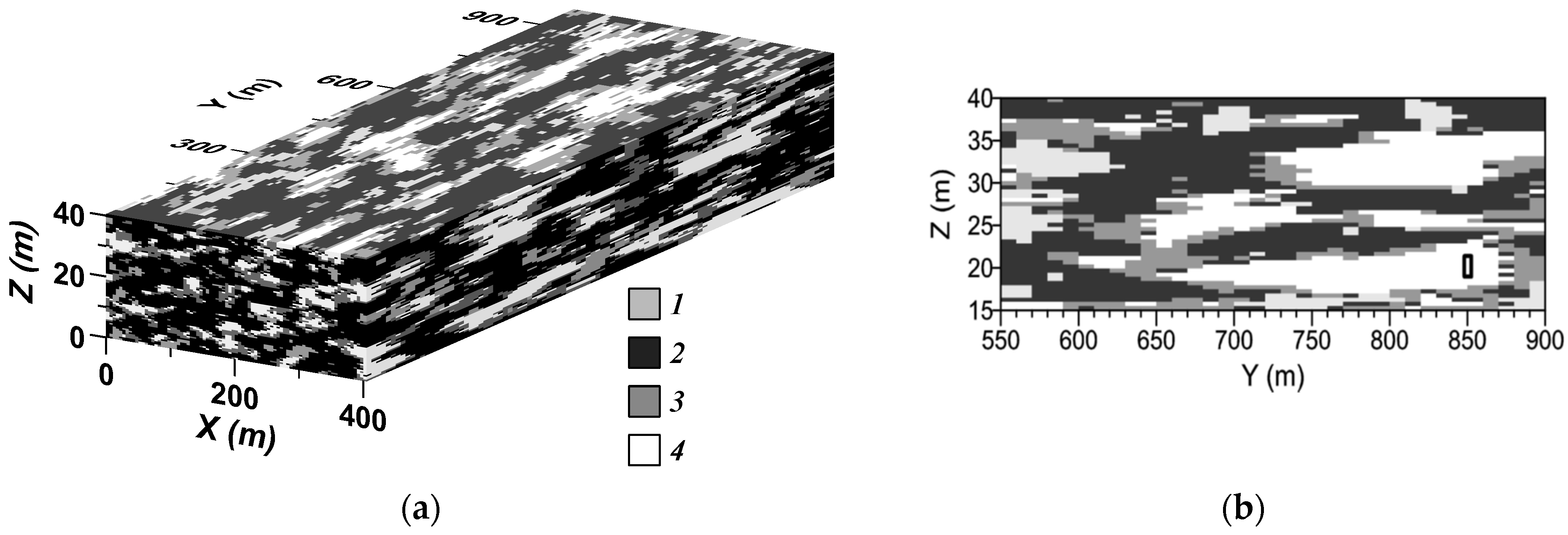
26]. The systematic behaviors of backward probabilities in three-dimensional natural geological media, such as regional-scale alluvial aquifer/aquitard systems, have not yet been reported in literature.
Fourth, the above-mentioned limitations question the commonly used assumption that the scale effect of backward probabilities can be ignored. In general, for a short (1.5 m for a commonly used short-screen) and narrow well surrounded by highly permeable sediments, researchers assumed that local dispersion around the well screen is negligible compared with the regional-scale dispersion occurring between the well and the contaminant source (see for example the particle tracking transport modeling conducted by Weissmann et al. [
14] using the middle interval of a well screen). Therefore, one conclusion is usually drawn and applied pervasively—the sample collected from either one interval, or the entire interval of a short screen, is representative of waters at any interval of the well screen. This assumption neglects the scale effect of backward probabilities, and quantitative evaluations are needed to support or correct it.
This study tries to fill the four knowledge gaps mentioned above. We develop the theoretical basis, improve the calculation algorithm, extend the application areas of backward probabilities, and quantitatively evaluate the scale effect of backward probabilities of contaminants in heterogeneous aquifer systems (notably, all natural aquifers are heterogeneous) in three steps. First, three different methods of particle moving, including the backward-in-time discrete random-walk (DRW) method, the backward-in-time continuous time random-walk (CTRW) method, and the particle mass balance method, are proposed and applied to derive the governing equation of backward location probability (BLP) and backward travel time probability (BTTP) of contaminants in groundwater flow systems. We show for the first time that, by tracking backward in time, the widely used random walk and mass balance theories can conveniently lead to backward probability models. Next, an improved backward-in-time RWPT technique is applied to solve the backward probabilities numerically. Finally, the effects of diameter, length, and depth of the well screen on BLP and BTTP are explored for a three-dimensional heterogeneous medium and its equivalent homogeneous counterpart using numerical solutions.
2. Governing Equations of Backward Probabilities
Backward probabilities of a particle, including BTTP and BLP, provide the probability of a particle at certain previous time(s) and location(s) given that the probability of the particle at the current time and location is 1. Specifically, BTTP describes the time required for the particle to travel from a known location to an observation point or area, and BLP describes the possible positions of the particle at a known time or period in the past.
The motion of a particle is well known to be composed of two processes: one is driven deterministically by a drift vector, and the other is driven by a Gaussian noise (or a non-Gaussian noise shown by our previous work [
25,
26]). This motion can be described by the following nonlinear Langevin equation, which is a stochastic differential equation modeling random dynamics driven by deterministic and fluctuating forces [
27]:
where
represents a Wiener process [
T1/2], and
denotes the particle’s displacement during time
. Interpreting Equation (3) in its integral version and applying the characteristics of Ito integration, one can use the following equation to describe the previous information of a particle given its current location and time:
A reliable backward model is the prerequisite for reliable applications of BLP/BTTP. In the following sub-sections, we derive Kolmogorov’s backward equation by solving the probability density function (PDF) of particles with displacements obeying Equation (4). For cross verification and extension purposes, three different methods are used.
2.1. Backward-in-Time Discrete Random-Walk (DRW) Method
The DRW method is first shown here because of its simplicity. For description simplicity, here we use a one-dimensional random walk (whose three-dimensional extension is straightforward). Let
denote the probability of a walker being at
after
steps in a one-dimensional random walk. Assuming that the individual steps of the random walk are independent and identically distributed, we have the following backward-in-time recurrence relationship:
where
denotes the probability that a walker who is currently at location
, moved from location
. Let
be the step size and
be the time interval between successive steps, and their limits toward zero; then, Equation (5) can be re-written as:
where
is the PDF for the walker located at
at time
.
Assuming
is differentiable once with respect to
and twice with respect to
, we can re-write Equation (6) using a formal Taylor expansion:
Because
, Equation (7) can be re-arranged to:
When and , the truncation error and becomes negligible.
We already know that:
where
is the
component of
, and
is the
-diagonal component of
[
5,
27]. They are also the two parameters used in the nonlinear Langevin equation [
27,
28,
29]. Dividing Equation (8) by
and inserting Equations (9) and (10) in Equation (8) leads to the following backward probability model:
2.2. Backward-in-Time Continuous Time Random-Walk (CTRW) Method
The CTRW method is considered here because it is theoretically stricter than the DRW method. There have been hundreds of papers discussing Brownian motion using CTRW (see for example, the review in [
30]), but most of them focus on the forward-in-time movement of particles. An in-depth introduction of the CTRW method can be found in the classical work of Metzler and Klafter [
31]. The Galilei variant/invariant assumptions, which might be disputable, sometimes are used to directly add an advection term to the diffusion equation [
31]. Here we extend the CTRW method in Metzler and Klafter [
31] for backward-in-time solutions and eliminate the Galilei variant/invariant assumptions.
The backward PDF is:
where
represents the backward increase in time with
,
denotes the PDF for particle reaching
at time
, and
is the PDF for particles without movement during the period of
to
. We use
and
to represent the detection location and time for forward-in-time formulations. The backward time is
, where
. The corresponding Fourier transform (with the symbol of hat ^) and Laplace transform (with the symbol of bar −) of Equation (12) is:
We then derive the expression of
and
. Considering the decoupled jump length and waiting time PDF [
31]:
where
is the Dirac delta function. Equation (14) is equal to:
where
is the waiting time PDF,
is the jump length PDF, and the symbol “*” denotes convolution. Taking both the Fourier and Laplace transforms for Equation (15), and then solving for
, we have:
Because
, the corresponding Laplace transform of
is:
Inserting Equations (16) and (17) into Equation (13) leads to:
To solve Equation (18), we first assume a Poissonian waiting time PDF [
31]:
where
is the mean waiting time and
> 0. We then assume that the particle jump size satisfies a Gaussian PDF (and the particle has different probabilities of directional particle movement for multi-dimensional extension). This allows particles to have a non-zero mean jump length
:
where
is the standard deviation of the random jump size.
The Laplace/Fourier transform of
and
is
and
, respectively. By inserting the first-order Taylor expansion of
and the second-order expansion of
into Equation (18), we have:
Assuming a long time and large space limit as in Metzler and Klafter [
31], we know that
is a higher order term than
, and
is a higher order term than
. Then we obtain the following equation using the reverse Laplace and Fourier transforms:
According to the relationship between the backward time and the increase in backward time, we can transfer Equation (22) to Equation (11), proving the backward probability model of Equation (11).
The above-mentioned random-walk-based methods indicate that the governing equation of the backward-in-time PDF has the same form as Kolmogorov’s backward equation. This result is not limited to one dimension because random walk methods can be extended to three dimensions [
2,
32,
33].
2.3. Method of Conservation of Particle Mass
The mass-balance method is proposed here for three-dimensional expansion. It is a reasonable assumption that each particle moves randomly in multiple dimensional spaces. For simplicity, we consider particle transport in the
direction first, and then we combine the spatial movements of each particle. Let
be the number of particles in cell
; then, the particle density in this cell is given by:
where
is the volume of cell
[
L3]. Assuming that the particle generally moves from cell
to cell
under ambient conditions, then the particle number flux from cell
to cell
per unit area and per unit time in the backward-in-time process is [
34]:
where the parameter
represents the difference in probabilities when particles jump forward and backward along
-axis, so
;
is the area of cell normal to
-axis [
L2];
is the number of jumps per unit time for each particle [
T−1]; and
is the cell length [
L]. Using the following Taylor series approximation:
we can then rewrite Equation (24) as:
When
, it is obvious that
. According to Fick’s law [
30],
. Equation (26) hence becomes:
For conservative solutes, the total number of particles remains stable during jumping events. The conservation of particle mass also means the conservation of the number of particles (which carry the solute mass or backward probability). Substituting Equation (27) into
, the mass conservation equation, and then expanding it to three dimensions, one obtains:
This formula extends Kolmogorov’s backward equation by showing that the vector
and tensor
, which control the advective and diffusive displacement of particles, do not necessarily have to be divergence free. This conclusion is consistent with the results of Neupauer and Wilson [
24] using the rigid, but mathematically complex, sensitivity-based adjoint approach. In the following we discuss whether this extension is reasonable in applications.
5. Discussion
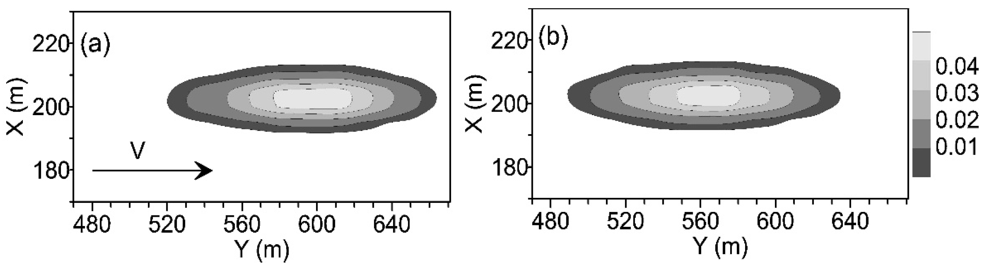
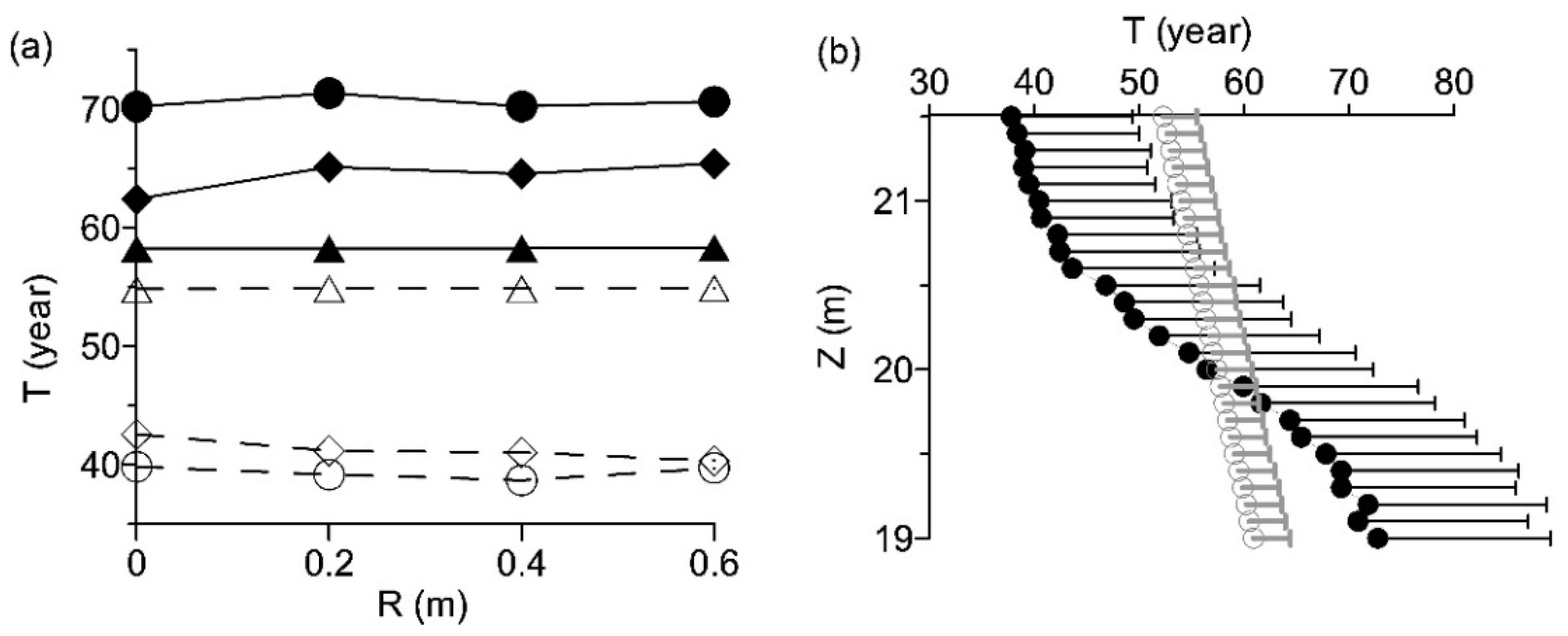
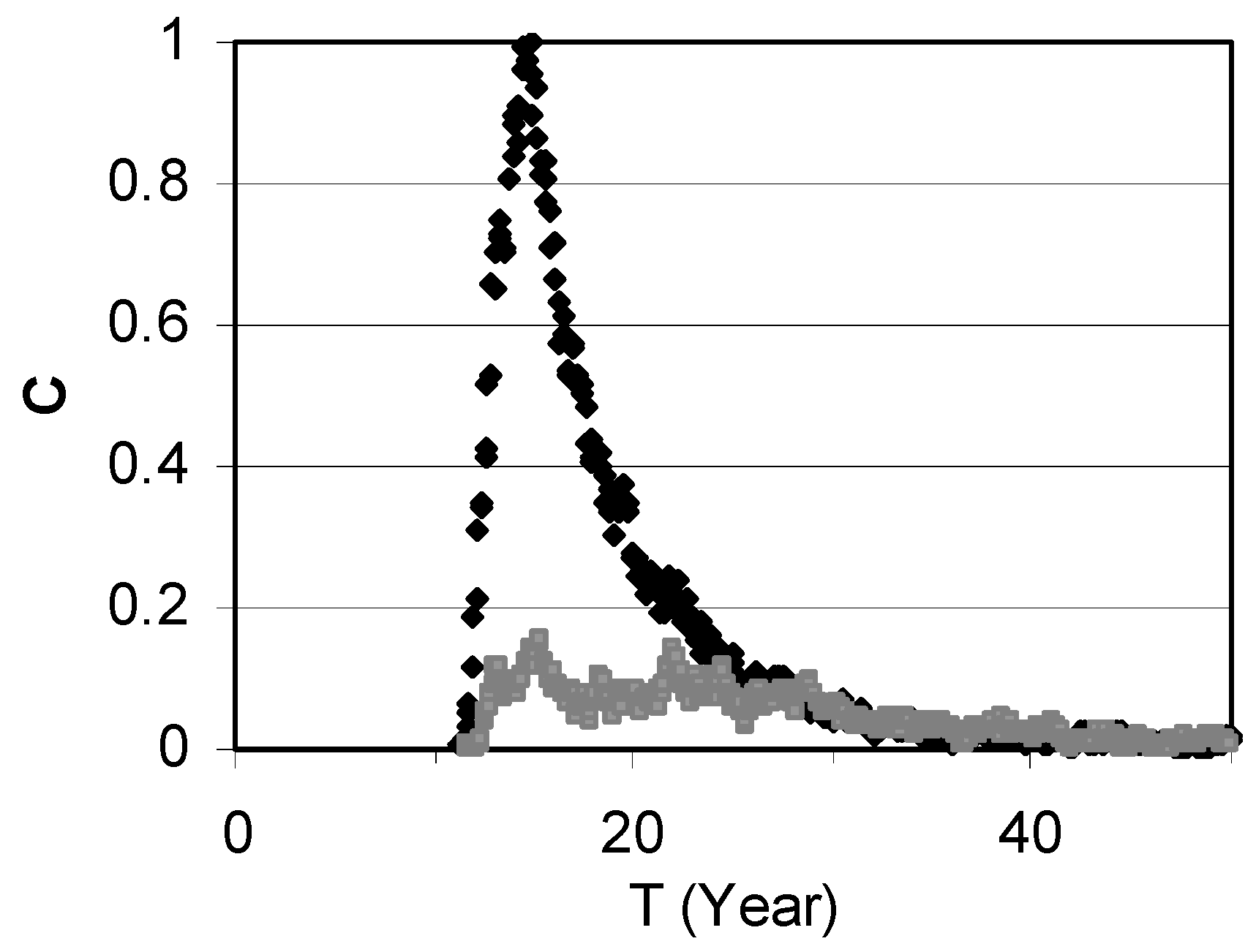
The major finding of this work (i.e., BLP and BTTP are sensitive to the vertical interval and length of well screens) has profound meanings for real-world applications where BTP and BTTP are used as critical indices. Specifically, the scale effect of backward probabilities can result in strong spatial and temporal variations in measured concentrations of groundwater samples, which thus raises serious questions in the current applications of backward probabilities, including the monitoring and evaluation of groundwater quality, identification of groundwater pollutant sources, assessment of aquifer vulnerability, and delineation of well-head protection zones. For instance, as indicated by
Figure 7, the normalized concentrations of contaminants measured at different depths along a short screen (2 m long) may vary up to 1 order of magnitude due to the scale effect of backward probabilities. This strong variation results in the following dilemma. If the monitoring network of groundwater quality is too sparse (a common scenario), it is difficult to capture variations in concentration within such a small local scale, and then it is most likely to miss the main characteristics of contaminant plumes. On the contrary, if the well screen is relatively long, a small amount of water collected from specific interval(s) of the well may not represent the aquifer where the well is. In both cases, it is important to evaluate the measurements based on the exact sampling location to obviate any misleading data. The method proposed by this study can be developed to assist field works, such as the design of monitoring networks.
As mentioned above, researchers simplify the heterogeneous aquifers for many reasons, such as lack of data or scale limitations. Comparisons in this study indicate the heterogeneous model has significantly different backward probabilities compared to the equivalent homogeneous and anisotropic models. However, our hydrogeologic interpretive skills have been strongly influenced by homogeneous conceptual models. We need to better understand the limitations of replacing a real-world heterogeneous medium by a homogeneous model when investigating backward probabilities, because the homogeneous model may be misleading.
This study therefore answered the four backward probability-related questions raised in Introduction. First, three particle-moving methods, namely, the backward DRW, backward CTRW, and particle mass balance, conveniently converted the forward-in-time transport model to its backward counterpart. Second, the backward conversion showed that the vector and the tensor in Kolmogorov’s backward equation need not to be divergence free. Third, the backward PDF properties were systematically analyzed for pollutants moving in a three-dimensional alluvial aquifer, whose nuance cannot be fully captured by its “equivalent” homogeneous model. Fourth and most importantly, extensive numerical experiments revealed the strong (vertical) scale effect of backward probability, challenging the commonly used assumption that the scale effect of backward probability is negligible for regional-scale natural aquifers.
Future extensions of this work are needed. For example, subsurface hydrodynamics and heterogeneity distributions influence the scale effect of backward probabilities and thus require further investigation. First, the main hydrodynamic conditions affecting the variations in backward probabilities include boundary conditions and transport parameters used in the simulation. Boundary conditions include the rate of recharge applied to the top boundary and horizontal flux from the upgradient boundary. Our preliminary results (not shown here) revealed that a larger recharge rate from the top boundary and/or a smaller flux from the upgradient boundary will cause smaller variations in backward probabilities along the well. In the models used by this study, the most important transport parameter is the molecular diffusion coefficient. A larger molecular diffusion coefficient may enhance leakage recharge from sediments having low permeability, resulting in more old components in the backward travel time probability distribution. Second, variation in the heterogeneity structure, such as the correlation length and the proportion of hydrofacies, may result in different preferential paths for both water and solute. Therefore, the heterogeneity structure may play an important role in the scale effect of backward probabilities. This topic will be further investigated in a future paper. Finally, the most important factor in a real-world application that may change the simulation results of this study is the actual distributions of depositional materials around the screened well. Sediments having low permeability may form mixed layers, such as clay laminae, within the highly permeable materials around the screen. The existence of low-permeability materials can enhance the difference in water intakes at different depths of the screen, and then enhance the scale effect of backward probabilities. One possible means to address this issue is to build and analyze multiple different but equally possible realizations for each scenario of hydrofacies models using the geostatistical tool applied above. The uncertainty of the calculated backward probabilities caused by the above factors deserves further research.
6. Conclusions
This study tried to fill the knowledge gaps of backward probabilities by building the governing equations and evaluating the scale effect of backward location and travel time probabilities for pollutants moving in a three-dimensional aquifer. Three main conclusions were drawn.
First, the governing equation of backward location probability and backward travel time probability cross-verified Kolmogorov’s backward equation and extended the theoretical basis of backward probabilities. The improved backward RWPT technique extended the application of backward probabilities to more complex, three-dimensional, heterogeneous alluvial settings. The groundwater flow field is not limited to steady-state conditions and the media do not have to have constant porosity values (see Equation (36), for example, where the velocity can be time dependent and the porosity can change in space).
Second, numerical experiments indicated that the backward probabilities are not sensitive to the well screen diameter, because the horizontal scale of the aquifer is much larger than the diameter of a well screen (hundreds of meters verses ~10
−1 to 10
0 m in this study). Therefore, a well can be simplified to be a vertical line inside an aquifer system during numerical modeling. Numerical simulations conducted by LaBolle et al. [
39] supported this conclusion by showing that the main behaviors of plume migrations were not significantly influenced by a limited variation in the initial horizontal location of contaminants.
Third, the backward location and travel time probabilities of groundwater contaminants can be significantly influenced by the variations in the vertical lengths of the well screen or the depths of sampling points along the well screen in complex heterogeneous aquifers. The results of this study showed that the backward probabilities of contaminants from one depth inside a 2.5 m long screen surrounded by highly permeable materials cannot represent the backward probabilities of contaminants in water packages entering the screen through another depth. Although the local dispersion around the well screen is negligible compared with the regional-scale dispersion occurring between the well and the source, groundwater can reach individual intervals of the same screen from different pathways connecting the water table and the well. Thus, the backward probabilities can change vertically, resulting in a scale effect of backward probabilities. The scale effect of backward probabilities may strongly affect real-world applications relying on BLP/BTTP.


