
The Spatial-Temporal Characteristics of Soil Moisture and Its Persistence over Australia in the Last 20 Years


Abstract
:1. Introduction
2. Materials and Methods
2.1. Study Area—Australia
2.2. Soil Moisture Datasets
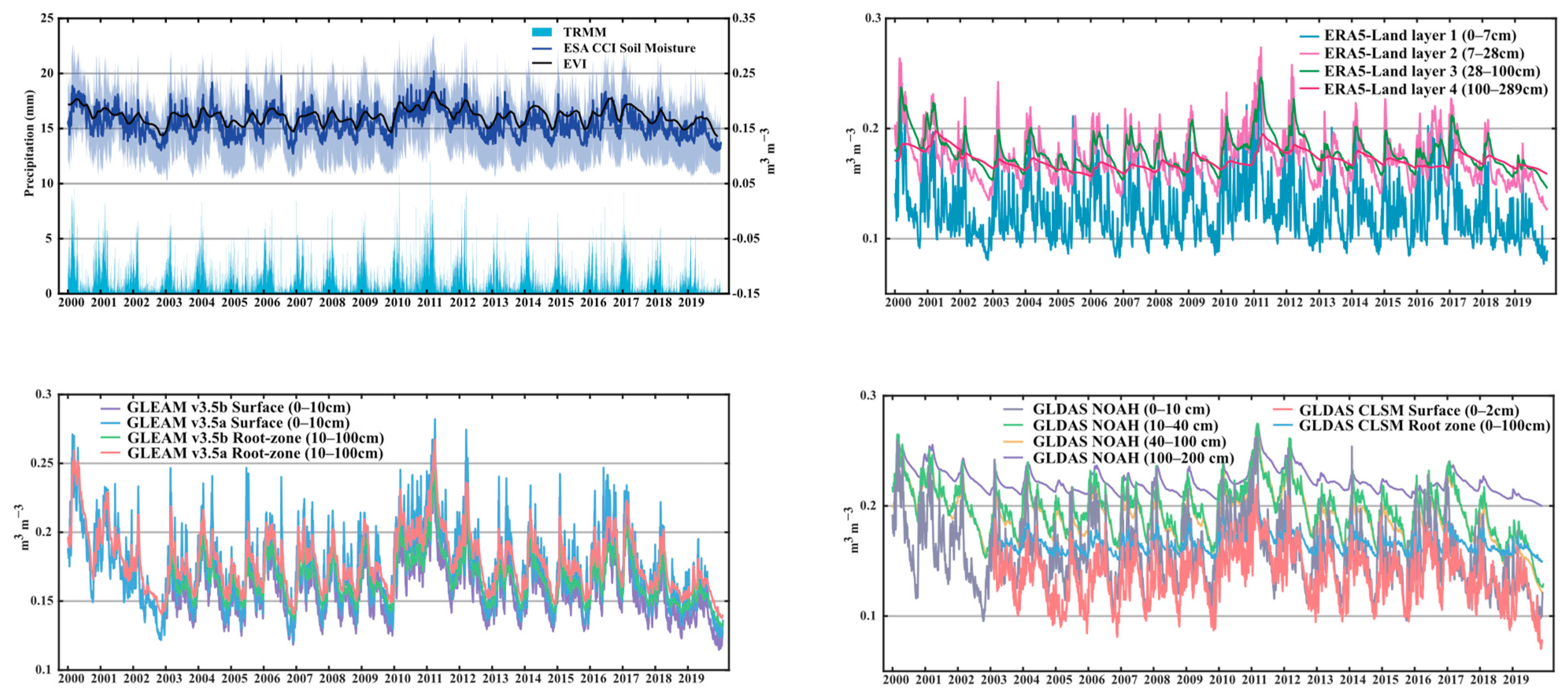
2.3. Other Auxiliary Data
2.4. Methods
2.4.1. Pearson Correlation
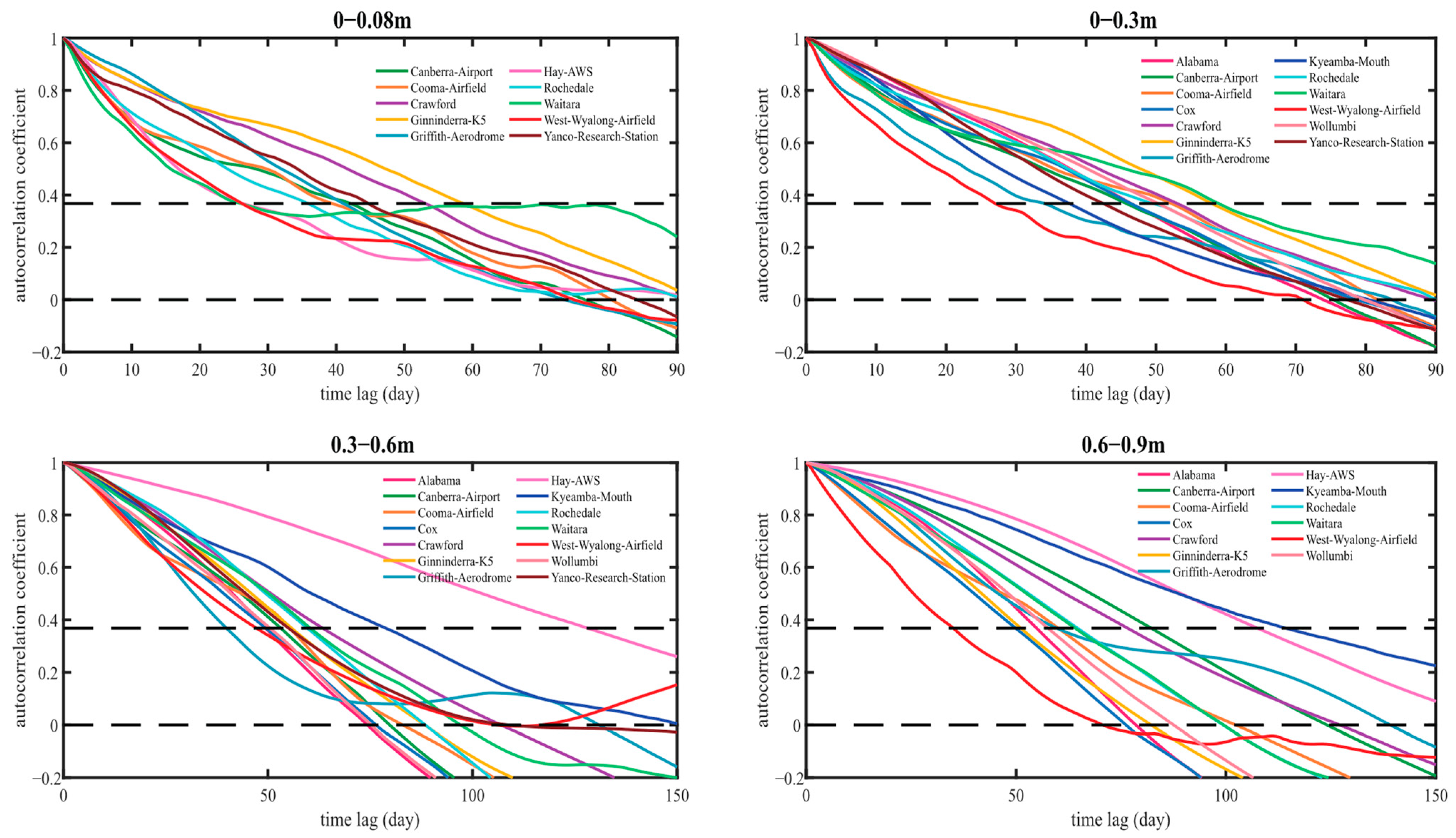
2.4.2. Autocorrelation (AC)
3. Results
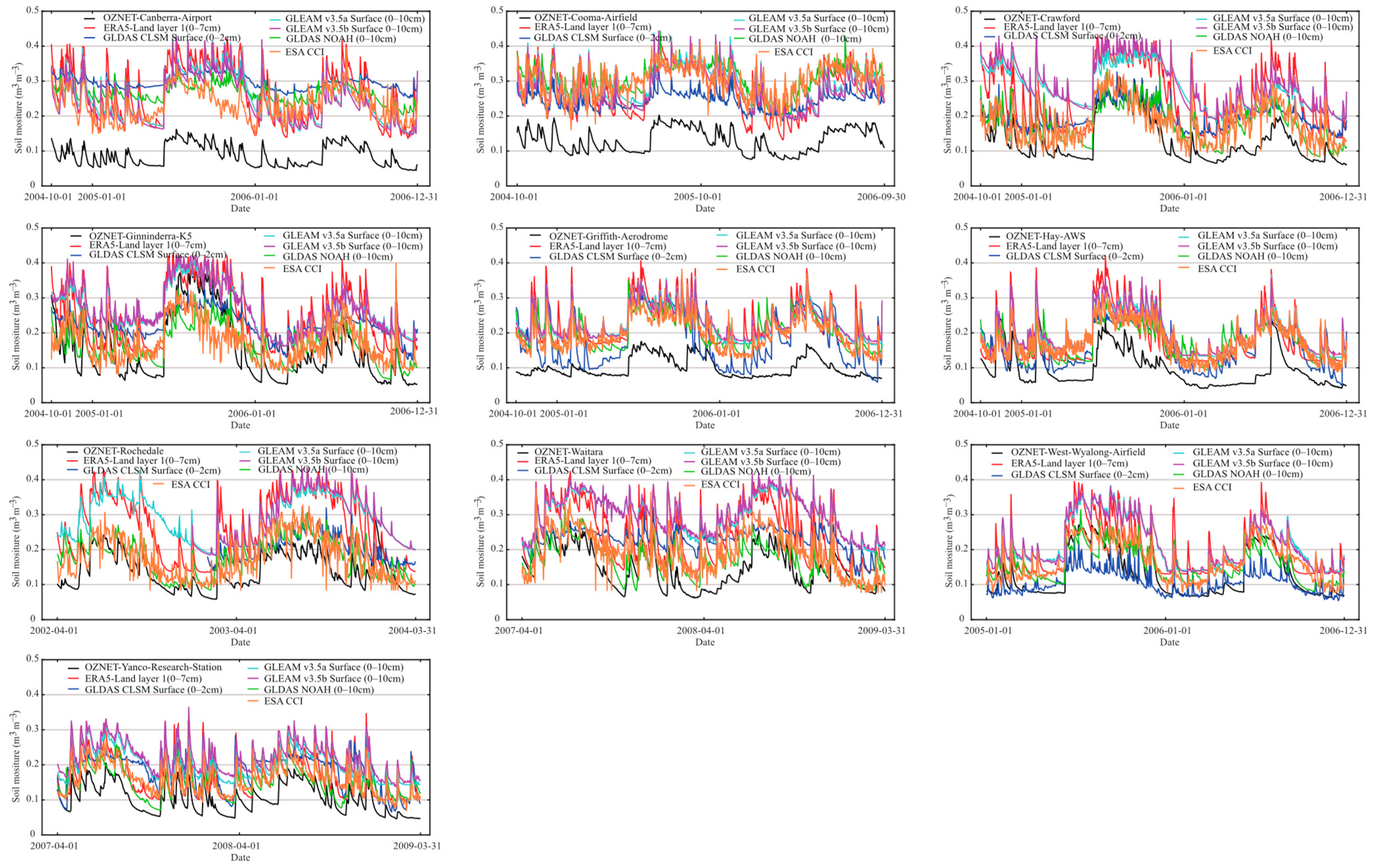
3.1. Evaluation of the Soil Moisture Data
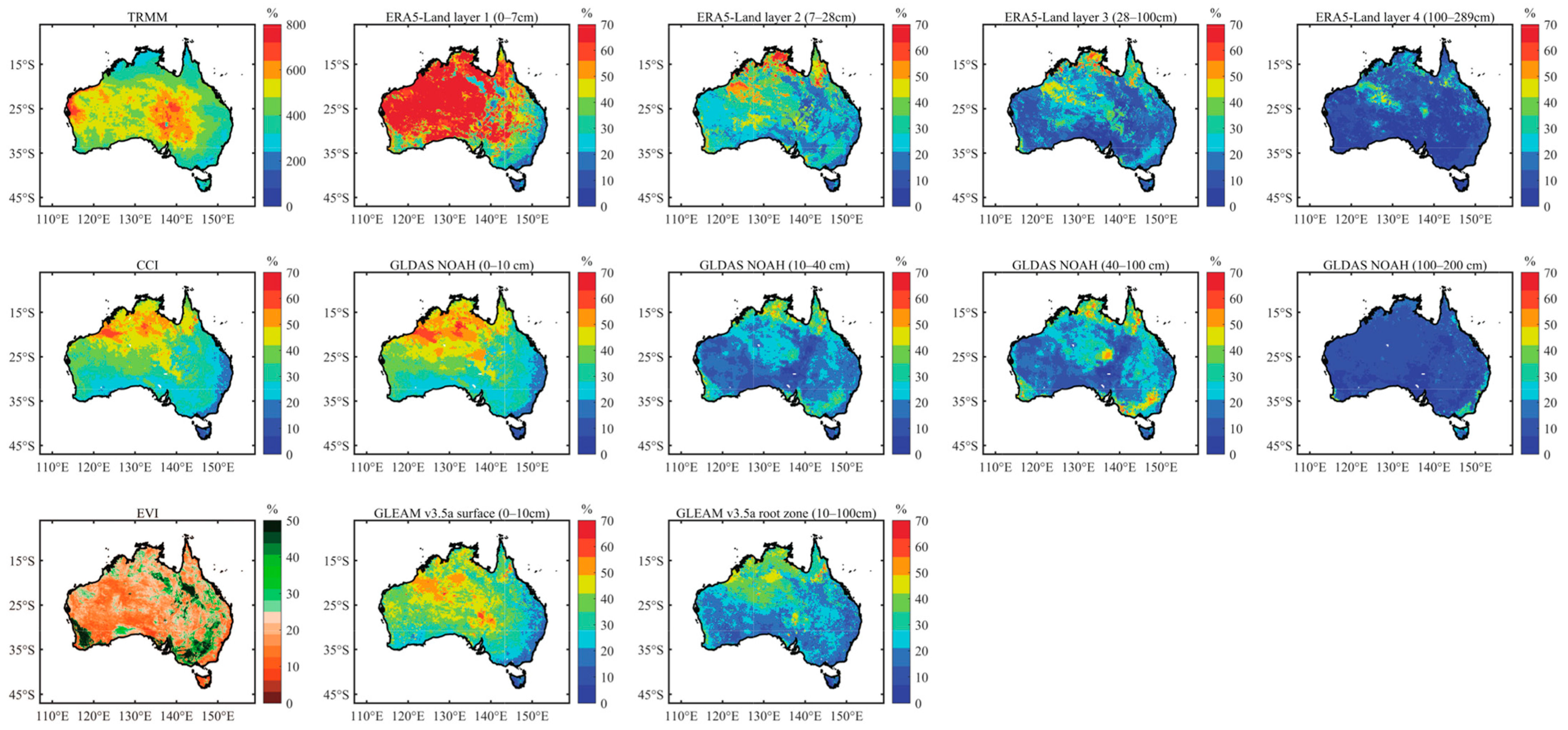
3.2. Temporal and Spatial Characteristics of Soil Moisture in Australia
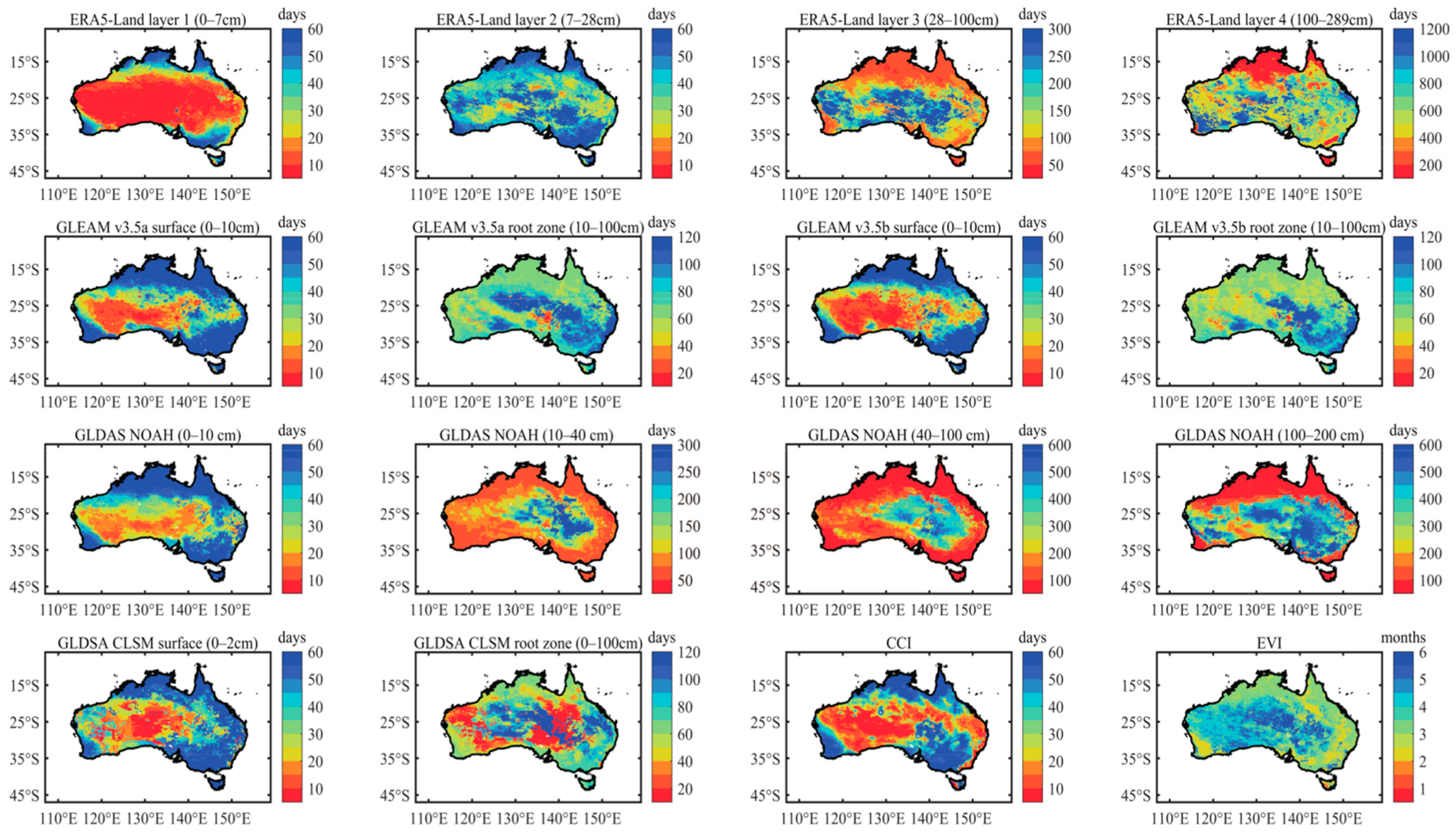
3.3. Soil Moisture Persistence in Australia
4. Discussion
4.1. The Wet and Dry Condition Indicated by SM
4.2. Possible Factors Affecting Surface SMP
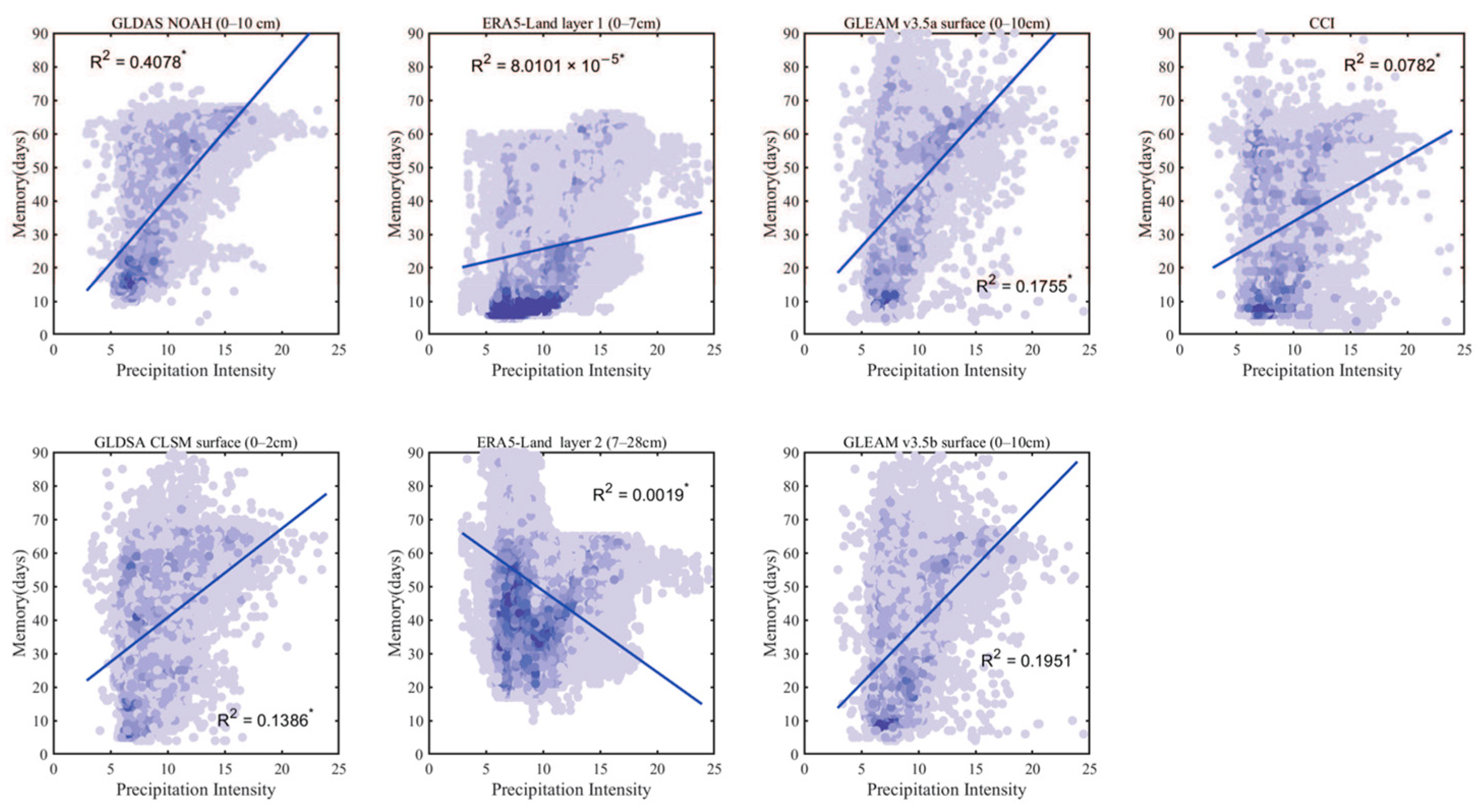
4.2.1. Relationship with Precipitation
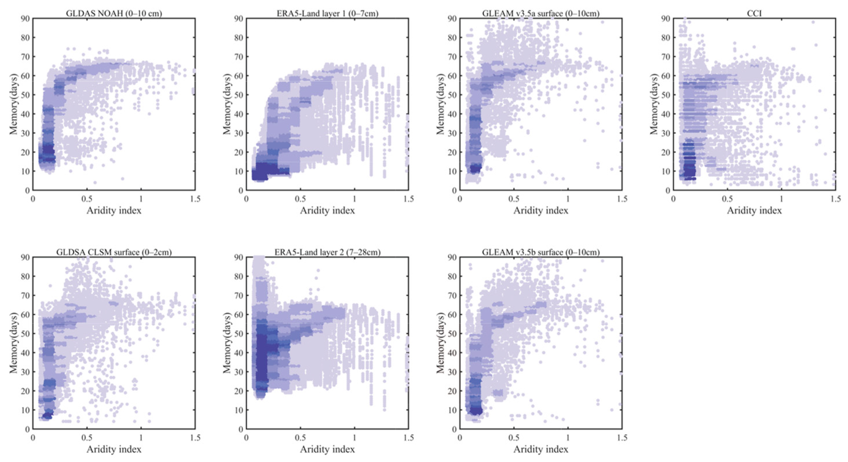
4.2.2. Relationship with Aridity
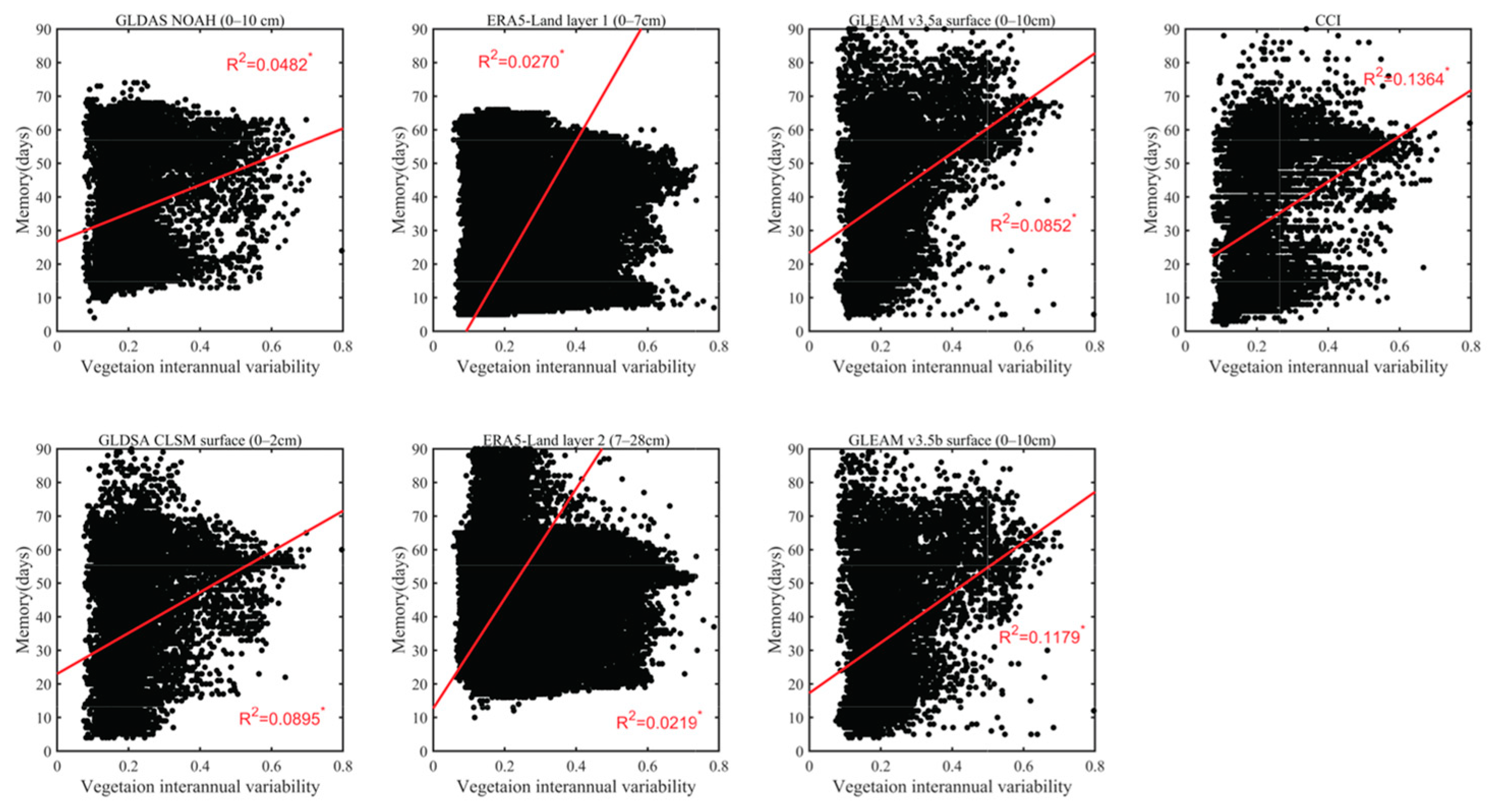
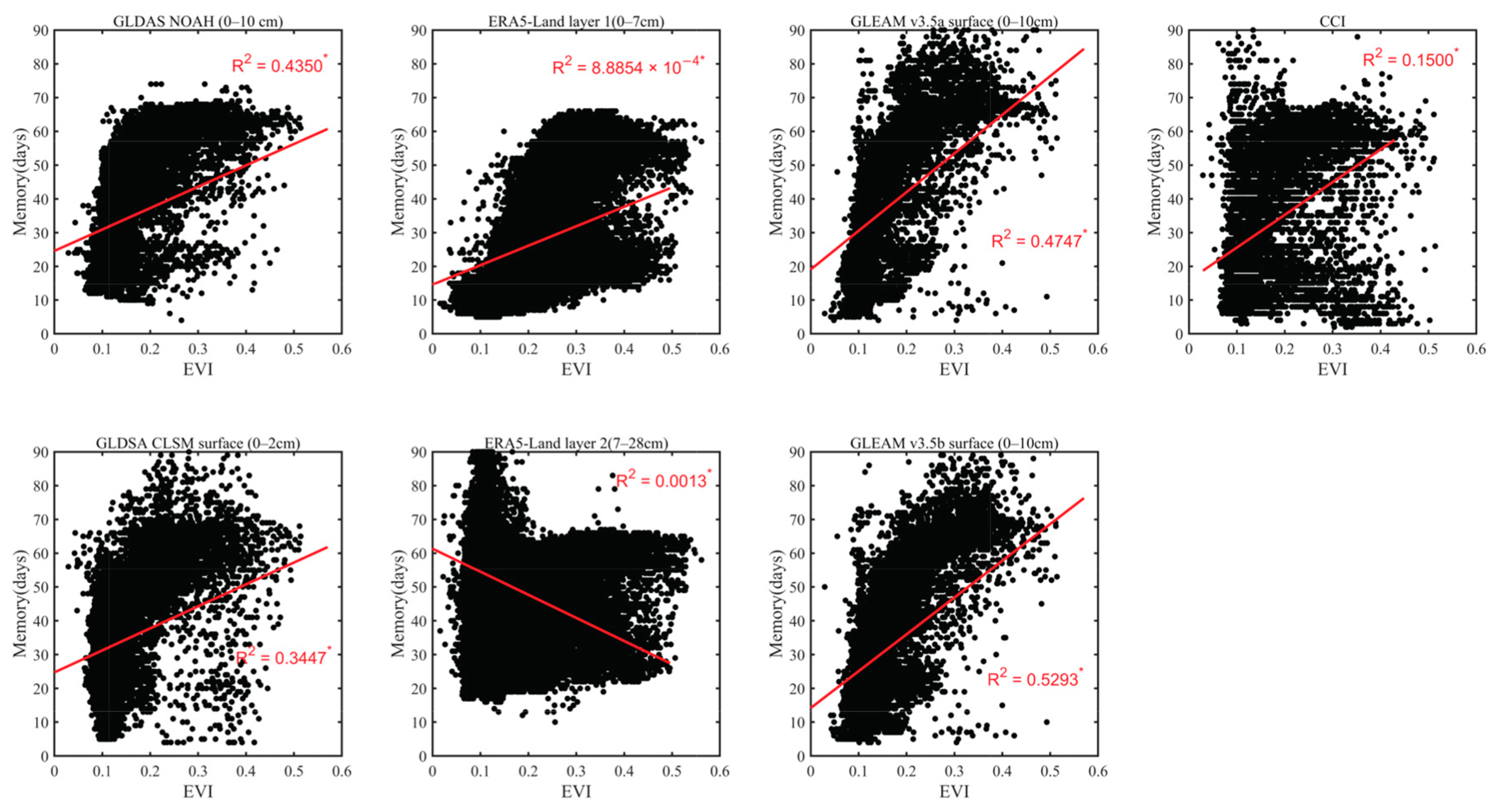
4.2.3. Relationship with Vegetation Status
5. Conclusions
Author Contributions
Funding
Institutional Review Board Statement
Informed Consent Statement
Data Availability Statement
Conflicts of Interest
Abbreviations
| AC | autocorrelation coefficient |
| AI | aridity index |
| CV | coefficient of variation |
| EVI | enhanced vegetation index |
| ET | evapotranspiration |
| ISMN | International Soil Moisture Network |
| LSMs | land surface models |
| NVIS-MVGs | National Vegetation Information System—Main Vegetation Groups |
| OZNET | Ozark Network Communications |
| PET | potential evapotranspiration |
| PF | precipitation frequency |
| PI | precipitation intensity |
| SM | soil moisture |
| SMP | soil moisture persistence |
| TRMM | Tropical Rainfall Measuring Mission |
Appendix A

| ISMN | ERA5-Land Layer 1 (0–7 cm) | GLDAS CLSM Surface (0–2 cm) | GLDAS NOAH (0–10 cm) | GLEAM v3.5a Surface (0–10 cm) | GLEAM v3.5b Surface (0–10 cm) | ESA CCI (<2 cm) | |
|---|---|---|---|---|---|---|---|
| Canberra_Airport | 43 | 34 (−9) | 56 (13) | 35 (−8) | 56 (13) | 53 (10) | 34 (−9) |
| Cooma_Airfield | 40 | 36 (−4) | 27 (−13) | 48 (8) | 56 (16) | 54 (14) | 12 (−28) |
| Crawford | 54 | 46 (−8) | 54 (0) | 42 (−12) | 64 (10) | 61 (7) | 42 (−12) |
| Ginninderra_K5 | 59 | 47 (−12) | 55 (−4) | 46 (−13) | 64 (5) | 62 (3) | 36 (−23) |
| Griffith_Aerodrome | 42 | 29 (−13) | 51 (9) | 34 (−8) | 43 (1) | 38 (−4) | 42 (0) |
| Hay_AWS | 27 | 38 (11) | 50 (23) | 36 (9) | 56 (29) | 44 (17) | 47 (20) |
| Rochedale | 36 | 57 (21) | - | 63 (27) | 62 (26) | - | 58 (22) |
| Waitara | 37 | 34 (−3) | 33 (−4) | 35 (−4) | 53 (16) | 52 (15) | 43 (6) |
| West_Wyalong_Airfield | 47 | 43 (−4) | 45 (−2) | 43 (−2) | 60 (13) | 57 (10) | 49 (2) |
| Yanco_Research_Station | 33 | 9 (−24) | 16 (−17) | 15 (−18) | 36 (3) | 36 (3) | 36 (3) |
| Average | 41.8 ± 9.6 | 37.3 ± 12.8 (−4.5 ± 12.6) | 43.0 ± 14.3 (0.6 ±12.6) | 39.7 ± 12.3 (−2.1 ± 13.4) | 55.0 ± 9.1 (13.2 ± 9.2) | 50.8 ± 9.4 (8.3 ± 6.8) | 39.9 ± 12.1 (−1.9 ± 16.4) |
References
- McColl, K.A.; He, Q.; Lu, H.; Entekhabi, D. Short-Term and Long-Term Surface Soil Moisture Memory Time Scales Are Spatially Anticorrelated at Global Scales. J. Hydrometeorol. 2019, 20, 1165–1182. [Google Scholar] [CrossRef]
- Rebel, K.T.; de Jeu, R.A.M.; Ciais, P.; Viovy, N.; Piao, S.L.; Kiely, G.; Dolman, A.J. A global analysis of soil moisture derived from satellite observations and a land surface model. Hydrol. Earth Syst. Sci. 2012, 16, 833–847. [Google Scholar] [CrossRef] [Green Version]
- Nicolai-Shaw, N.; Gudmundsson, L.; Hirschi, M.; Seneviratne, S. Long-term predictability of soil moisture dynamics at the global scale: Persistence versus large-scale drivers. Geophys. Res. Lett. 2016, 43, 8554–8562. [Google Scholar] [CrossRef] [Green Version]
- Ahmadalipour, A.; Moradkhani, H.; Yan, H.; Zarekarizi, M. Remote Sensing of Drought: Vegetation, Soil Moisture, and Data Assimilation. In Remote Sensing of Hydrological Extremes. Springer Remote Sensing/Photogrammetry; Lakshmi, V., Ed.; Springer: Cham, Switzerland, 2017; pp. 121–149. [Google Scholar] [CrossRef]
- Al-Yaari, A.; Wigneron, J.-P.; Dorigo, W.; Colliander, A.; Pellarin, T.; Hahn, S.; Mialon, A.; Richaume, P.; Moran, R.F.; Fan, L.; et al. Assessment and inter-comparison of recently developed/reprocessed microwave satellite soil moisture products using ISMN ground-based measurements. Remote Sens. Environ. 2019, 224, 289–303. [Google Scholar] [CrossRef]
- Yan, Q.; Huang, W.; Jin, S.; Jia, Y. Pan-tropical soil moisture mapping based on a three-layer model from CYGNSS GNSS-R data. Remote Sens. Environ. 2020, 247, 111944. [Google Scholar] [CrossRef]
- Qian, T.; Dai, A.; Trenberth, K.E.; Oleson, K.W. Simulation of Global Land Surface Conditions from 1948 to 2004. Part I: Forcing Data and Evaluations. J. Hydrometeorol. 2006, 7, 953–975. [Google Scholar] [CrossRef]
- Huang, Y.; Yu, X.; Li, E.; Chen, H.; Li, L.; Wu, X.; Li, X. A process-based water balance model for semi-arid ecosystems: A case study of psammophytic ecosystems in Mu Us Sandland, Inner Mongolia, China. Ecol. Model. 2017, 353, 77–85. [Google Scholar] [CrossRef] [Green Version]
- Elshorbagy, A.; Parasuraman, K. On the relevance of using artificial neural networks for estimating soil moisture content. J. Hydrol. 2008, 362, 1–18. [Google Scholar] [CrossRef]
- Wen, H.; Brantley, S.L.; Davis, K.J.; Duncan, J.M.; Li, L. The Limits of Homogenization: What Hydrological Dynamics can a Simple Model Represent at the Catchment Scale? Water Resour. Res. 2021, 57. [Google Scholar] [CrossRef]
- Mao, Y.; Crow, W.T.; Nijssen, B. A Unified Data-Driven Method to Derive Hydrologic Dynamics From Global SMAP Surface Soil Moisture and GPM Precipitation Data. Water Resour. Res. 2020, 56. [Google Scholar] [CrossRef]
- Wang, Y.; Yang, J.; Chen, Y.; De Maeyer, P.; Li, Z.; Duan, W. Detecting the Causal Effect of Soil Moisture on Precipitation Using Convergent Cross Mapping. Sci. Rep. 2018, 8, 12171. [Google Scholar] [CrossRef] [PubMed]
- Tuttle, S.E.; Salvucci, G.D. Confounding factors in determining causal soil moisture-precipitation feedback. Water Resour. Res. 2017, 53, 5531–5544. [Google Scholar] [CrossRef]
- Tuttle, S.; Salvucci, G. Empirical evidence of contrasting soil moisture–precipitation feedbacks across the United States. Science 2016, 352, 825–828. [Google Scholar] [CrossRef] [Green Version]
- Sun, S.; Wang, G. The complexity of using a feedback parameter to quantify the soil moisture-precipitation relationship. J. Geophys. Res. Earth Surf. 2012, 117, 11113. [Google Scholar] [CrossRef] [Green Version]
- Eltahir, E.A.B. A Soil Moisture-Rainfall Feedback Mechanism: 1. Theory and observations. Water Resour. Res. 1998, 34, 765–776. [Google Scholar] [CrossRef]
- Jacobs, E.M.; Bertassello, L.E.; Rao, P.S.C. Drivers of regional soil water storage memory and persistence. Vadose Zone J. 2020, 19, e20050. [Google Scholar] [CrossRef]
- Kidron, G.J. Comparing overland flow processes between semiarid and humid regions: Does saturation overland flow take place in semiarid regions? J. Hydrol. 2021, 593, 125624. [Google Scholar] [CrossRef]
- Chen, T.; de Jeu, R.; Liu, Y.; van der Werf, G.; Dolman, A. Using satellite based soil moisture to quantify the water driven variability in NDVI: A case study over mainland Australia. Remote Sens. Environ. 2014, 140, 330–338. [Google Scholar] [CrossRef]
- Su, C.-H.; Zhang, J.; Gruber, A.; Parinussa, R.; Ryu, D.; Crow, W.T.; Wagner, W. Error decomposition of nine passive and active microwave satellite soil moisture data sets over Australia. Remote Sens. Environ. 2016, 182, 128–140. [Google Scholar] [CrossRef]
- Dorigo, W.A.; Wagner, W.; Hohensinn, R.; Hahn, S.; Paulik, C.; Xaver, A.; Gruber, A.; Drusch, M.; Mecklenburg, S.; van Oevelen, P.; et al. The International Soil Moisture Network: A data hosting facility for global in situ soil moisture measurements. Hydrol. Earth Syst. Sci. 2011, 15, 1675–1698. [Google Scholar] [CrossRef] [Green Version]
- Sandiford, M.; Lawrie, K.; Brodie, R.S. Hydrogeological implications of active tectonics in the Great Artesian Basin, Australia. Appl. Hydrogeol. 2020, 28, 57–73. [Google Scholar] [CrossRef]
- Chen, T.; McVicar, T.R.; Wang, G.; Chen, X.; De Jeu, R.A.M.; Liu, Y.Y.; Shen, H.; Zhang, F.; Dolman, A.J. Advantages of Using Microwave Satellite Soil Moisture over Gridded Precipitation Products and Land Surface Model Output in Assessing Regional Vegetation Water Availability and Growth Dynamics for a Lateral Inflow Receiving Landscape. Remote Sens. 2016, 8, 428. [Google Scholar] [CrossRef] [Green Version]
- Abram, N.J.; Henley, B.J.; Gupta, A.S.; Lippmann, T.J.R.; Clarke, H.; Dowdy, A.J.; Sharples, J.J.; Nolan, R.H.; Zhang, T.; Wooster, M.J.; et al. Connections of climate change and variability to large and extreme forest fires in southeast Australia. Commun. Earth Environ. 2021, 2, 1–17. [Google Scholar] [CrossRef]
- Miralles, D.G.; Nieto, R.; McDowell, N.G.; Dorigo, W.; Verhoest, N.E.; Liu, Y.Y.; Teuling, A.; Dolman, A.; Good, S.P.; Gimeno, L. Contribution of water-limited ecoregions to their own supply of rainfall. Environ. Res. Lett. 2016, 11, 124007. [Google Scholar] [CrossRef]
- Harris, R.M.B.; Beaumont, L.J.; Vance, T.R.; Tozer, C.R.; Remenyi, T.; Perkins-Kirkpatrick, S.E.; Mitchell, P.; Nicotra, A.; McGregor, S.; Andrew, N.R.; et al. Biological responses to the press and pulse of climate trends and extreme events. Nat. Clim. Chang. 2018, 8, 579–587. [Google Scholar] [CrossRef]
- Dorigo, W.; Wagner, W.; Albergel, C.; Albrecht, F.; Balsamo, G.; Brocca, L.; Chung, D.; Ertl, M.; Forkel, M.; Gruber, A.; et al. ESA CCI Soil Moisture for improved Earth system understanding: State-of-the art and future directions. Remote Sens. Environ. 2017, 203, 185–215. [Google Scholar] [CrossRef]
- Gruber, A.; Scanlon, T.; van der Schalie, R.; Wagner, W.; Dorigo, W. Evolution of the ESA CCI Soil Moisture climate data records and their underlying merging methodology. Earth Syst. Sci. Data 2019, 11, 717–739. [Google Scholar] [CrossRef] [Green Version]
- Muñoz-Sabater, J.; Dutra, E.; Agustí-Panareda, A.; Albergel, C.; Arduini, G.; Balsamo, G.; Boussetta, S.; Choulga, M.; Harrigan, S.; Hersbach, H.; et al. ERA5-Land: A state-of-the-art global reanalysis dataset for land applications. Earth Syst. Sci. Data 2021, 13, 4349–4383. [Google Scholar] [CrossRef]
- Li, B.; Rodell, M.; Kumar, S.; Beaudoing, H.K.; Getirana, A.; Zaitchik, B.F.; De Goncalves, L.G.; Cossetin, C.; Bhanja, S.; Mukherjee, A.; et al. Global GRACE Data Assimilation for Groundwater and Drought Monitoring: Advances and Challenges. Water Resour. Res. 2019, 55, 7564–7586. [Google Scholar] [CrossRef] [Green Version]
- Rodell, M.; Houser, P.R.; Jambor, U.; Gottschalck, J.; Mitchell, K.; Meng, C.-J.; Arsenault, K.; Cosgrove, B.; Radakovich, J.; Arsenault, K.; et al. The Global Land Data Assimilation System. Bull. Am. Meteorol. Soc. 2004, 85, 381–394. [Google Scholar] [CrossRef] [Green Version]
- Miralles, D.G.; Holmes, T.R.H.; De Jeu, R.A.M.; Gash, J.H.; Meesters, A.G.C.A.; Dolman, A.J. Global land-surface evaporation estimated from satellite-based observations. Hydrol. Earth Syst. Sci. 2011, 15, 453–469. [Google Scholar] [CrossRef] [Green Version]
- Martens, B.; Gonzalez Miralles, D.; Lievens, H.; Van Der Schalie, R.; De Jeu, R.A.M.; Fernández-Prieto, D.; Beck, H.E.; Dorigo, W.A.; Verhoest, N.E.C. GLEAM v3: Satellite-based land evaporation and root-zone soil moisture. Geosci. Model Dev. 2017, 10, 1903–1925. [Google Scholar] [CrossRef] [Green Version]
- Harris, I.; Osborn, T.J.; Jones, P.; Lister, D. Version 4 of the CRU TS monthly high-resolution gridded multivariate climate dataset. Sci. Data 2020, 7, 1–18. [Google Scholar] [CrossRef] [PubMed] [Green Version]
- Hulme, M. Recent Climatic Change in the World’s Drylands. Geophys. Res. Lett. 1996, 23, 61–64. [Google Scholar] [CrossRef]
- Huang, J.; Li, Y.; Fu, C.; Chen, F.; Fu, Q.; Dai, A.; Shinoda, M.; Ma, Z.; Guo, W.; Li, Z.; et al. Dryland climate change: Recent progress and challenges. Rev. Geophys. 2017, 55, 719–778. [Google Scholar] [CrossRef]
- Xu, H.; Wang, X.; Zhao, C.; Yang, X. Assessing the response of vegetation photosynthesis to meteorological drought across northern China. Land Degrad. Dev. 2021, 32, 20–34. [Google Scholar] [CrossRef]
- Huffman, G.J.; Bolvin, D.T.; Nelkin, E.J.; Wolff, D.B.; Adler, R.F.; Gu, G.; Hong, Y.; Bowman, K.P.; Stocker, E.F. The TRMM Multisatellite Precipitation Analysis (TMPA): Quasi-Global, Multiyear, Combined-Sensor Precipitation Estimates at Fine Scales. J. Hydrometeorol. 2007, 8, 38–55. [Google Scholar] [CrossRef]
- Eamus, D.; Huete, A.; Cleverly, J.; Nolan, R.; Ma, X.; Tarin, T.; Santini, N. Mulga, a major tropical dry open forest of Australia: Recent insights to carbon and water fluxes. Environ. Res. Lett. 2016, 11, 125011. [Google Scholar] [CrossRef] [Green Version]
- Delworth, T.; Manabe, S. The Influence of Potential Evaporation on the Variabilities of Simulated Soil Wetness and Climate. J. Clim. 1988, 1, 523–547. [Google Scholar] [CrossRef]
- Greve, P.; Orlowsky, B.; Mueller, B.; Sheffield, J.; Reichstein, M.; Seneviratne, S. Global assessment of trends in wetting and drying over land. Nat. Geosci. 2014, 7, 716–721. [Google Scholar] [CrossRef]
- Deng, Y.; Wang, S.; Bai, X.; Luo, G.; Wu, L.; Chen, F.; Wang, J.; Li, C.; Yang, Y.; Hu, Z.; et al. Vegetation greening intensified soil drying in some semi-arid and arid areas of the world. Agric. For. Meteorol. 2020, 292–293, 108103. [Google Scholar] [CrossRef]
- McColl, K.A.; Alemohammad, S.H.; Akbar, R.; Konings, A.G.; Yueh, S.; Entekhabi, D. The global distribution and dynamics of surface soil moisture. Nat. Geosci. 2017, 10, 100–104. [Google Scholar] [CrossRef]
- McColl, K.A.; Wang, W.; Peng, B.; Akbar, R.; Gianotti, D.J.S.; Lu, H.; Pan, M.; Entekhabi, D. Global characterization of surface soil moisture drydowns. Geophys. Res. Lett. 2017, 44, 3682–3690. [Google Scholar] [CrossRef]
- IPCC. Climate Change 2021: The Physical Science Basis. Contribution of Working Group I to the Sixth Assessment Report of the Intergovernmental Panel on Climate Change; Masson-Delmotte, V., Zhai, P., Pirani, A., Connors, S.L., Péan, C., Berger, S., Caud, N., Chen, Y., Goldfarb, L., Gomis, M.I., et al., Eds.; Cambridge University Press: Cambridge, UK, 2021; in press. [Google Scholar]
- Xie, Z.; Huete, A.; Cleverly, J.; Phinn, S.; McDonald-Madden, E.; Cao, Y.; Qin, F. Multi-climate mode interactions drive hydrological and vegetation responses to hydroclimatic extremes in Australia. Remote Sens. Environ. 2019, 231, 111270. [Google Scholar] [CrossRef]
- Xie, Z.; Huete, A.; Restrepo-Coupe, N.; Ma, X.; Devadas, R.; Caprarelli, G. Spatial partitioning and temporal evolution of Australia’s total water storage under extreme hydroclimatic impacts. Remote Sens. Environ. 2016, 183, 43–52. [Google Scholar] [CrossRef]
- Ivanov, V.Y.; Bras, R.L.; Vivoni, E.R. Vegetation-hydrology dynamics in complex terrain of semiarid areas: 1. A mechanistic approach to modeling dynamic feedbacks. Water Resour. Res. 2008, 44. [Google Scholar] [CrossRef] [Green Version]
- Cook, B.I.; Bonan, G.B.; Levis, S. Soil Moisture Feedbacks to Precipitation in Southern Africa. J. Clim. 2006, 19, 4198–4206. [Google Scholar] [CrossRef] [Green Version]
- Li, X.-Y. Mechanism of coupling, response and adaptation between soil, vegetation and hydrology in arid and semiarid regions. Sci. Sin. Terrae 2011, 41, 1721–1730. [Google Scholar]
- Ford, T.W.; Quiring, S.M.; Thakur, B.; Jogineedi, R.; Houston, A.; Yuan, S.; Kalra, A.; Lock, N. Evaluating Soil Moisture—Precipitation Interactions Using Remote Sensing: A Sensitivity Analysis. J. Hydrometeorol. 2018, 19, 1237–1253. [Google Scholar] [CrossRef]
- Cheng, Y.; Chan, P.W.; Wei, X.; Hu, Z.; Kuang, Z.; McColl, K.A. Soil Moisture Control of Precipitation Reevaporation over a Heterogeneous Land Surface. J. Atmos. Sci. 2021, 78, 3369–3383. [Google Scholar] [CrossRef]
- Guswa, A.J. Canopy vs. Roots: Production and Destruction of Variability in Soil Moisture and Hydrologic Fluxes. Vadose Zone J. 2012, 11, vzj2011.0159. [Google Scholar] [CrossRef] [Green Version]
- He, Q.; Yue, S.; Lu, H.; Liu, Z.; Huang, X.; Entekhabi, D. Identifying Terrestrial Vegetation-Soil Moisture Oscillation from Satellite Observations. In Proceedings of the IGARSS 2020—2020 IEEE International Geoscience and Remote Sensing Symposium, Waikoloa, HI, USA, 26 September–2 October 2020; pp. 4570–4573. [Google Scholar]
- Aeruo, G.; Velicogna, I.; Kimball, J.S.; Du, J.; Kim, Y.; Colliander, A.; Njoku, E. Satellite-observed changes in vegetation sensitivities to surface soil moisture and total water storage variations since the 2011 Texas drought. Environ. Res. Lett. 2017, 12, 054006. [Google Scholar] [CrossRef] [Green Version]


| Data | Data Type | Layers | Temporal Coverage | Spatial Resolution | Temporal Resolution |
|---|---|---|---|---|---|
| ERA5-Land | Reanalysis | 0.00–0.07 m, 0.07–0.28 m, 0.28–1.00 m, 1.00–2.89 m | 1950–Present | 0.1° | 1 h |
| GLDAS CLSM | Land model | 0.00–0.02 m, 0.00–1.00 m | February 2003–July 2021 | 0.25° | 1 d |
| GLDAS NOAH | Land model | 0.00–0.10 m, 0.10–0.40 m, 0.40–1.00 m, 1.00–2.00 m | January 2000–July 2021 | 0.25° | 3 h |
| GLEAM v3.5a | Land model | 0.00–0.10 m, 0.10–1.00 m | 1980–2020 | 0.25° | 1 d |
| GLEAM v3.5b | Land model | 0.00–0.10 m, 0.10–1.00 m | January 2003–July 2020 | 0.25° | 1 d |
| ESA CCI | Remote sensing | <0.02 m | 1979–2019 | 0.25° | 1 d |
| Sites | ERA5-Land Layer 1 (0–7 cm) | GLDAS CLSM Surface (0–2 cm) | GLDAS NOAH (0–10 cm) | GLEAM v3.5a Surface (0–10 cm) | GLEAM v3.5b Surface (0–10 cm) | ESA CCI (<2 cm) |
|---|---|---|---|---|---|---|
| Canberra_Airport | 0.88 | 0.76 | 0.76 | 0.79 | 0.82 | 0.84 |
| Cooma_Airfield | 0.88 | 0.77 | 0.77 | 0.83 | 0.84 | 0.72 |
| Crawford | 0.88 | 0.84 | 0.79 | 0.82 | 0.86 | 0.77 |
| Ginninderra_K5 | 0.89 | 0.85 | 0.81 | 0.89 | 0.88 | 0.74 |
| Griffith_Aerodrome | 0.72 | 0.73 | 0.67 | 0.80 | 0.80 | 0.73 |
| Hay_AWS | 0.71 | 0.68 | 0.69 | 0.73 | 0.73 | 0.65 |
| Rochedale | 0.78 | - | 0.67 | 0.71 | - | 0.70 |
| Waitara | 0.81 | 0.59 | 0.74 | 0.68 | 0.69 | 0.71 |
| West_Wyalong_Airfield | 0.88 | 0.75 | 0.85 | 0.90 | 0.91 | 0.88 |
| Yanco_Research_Station | 0.85 | 0.71 | 0.74 | 0.84 | 0.87 | 0.84 |
| Average | 0.83 | 0.74 | 0.75 | 0.80 | 0.82 | 0.76 |
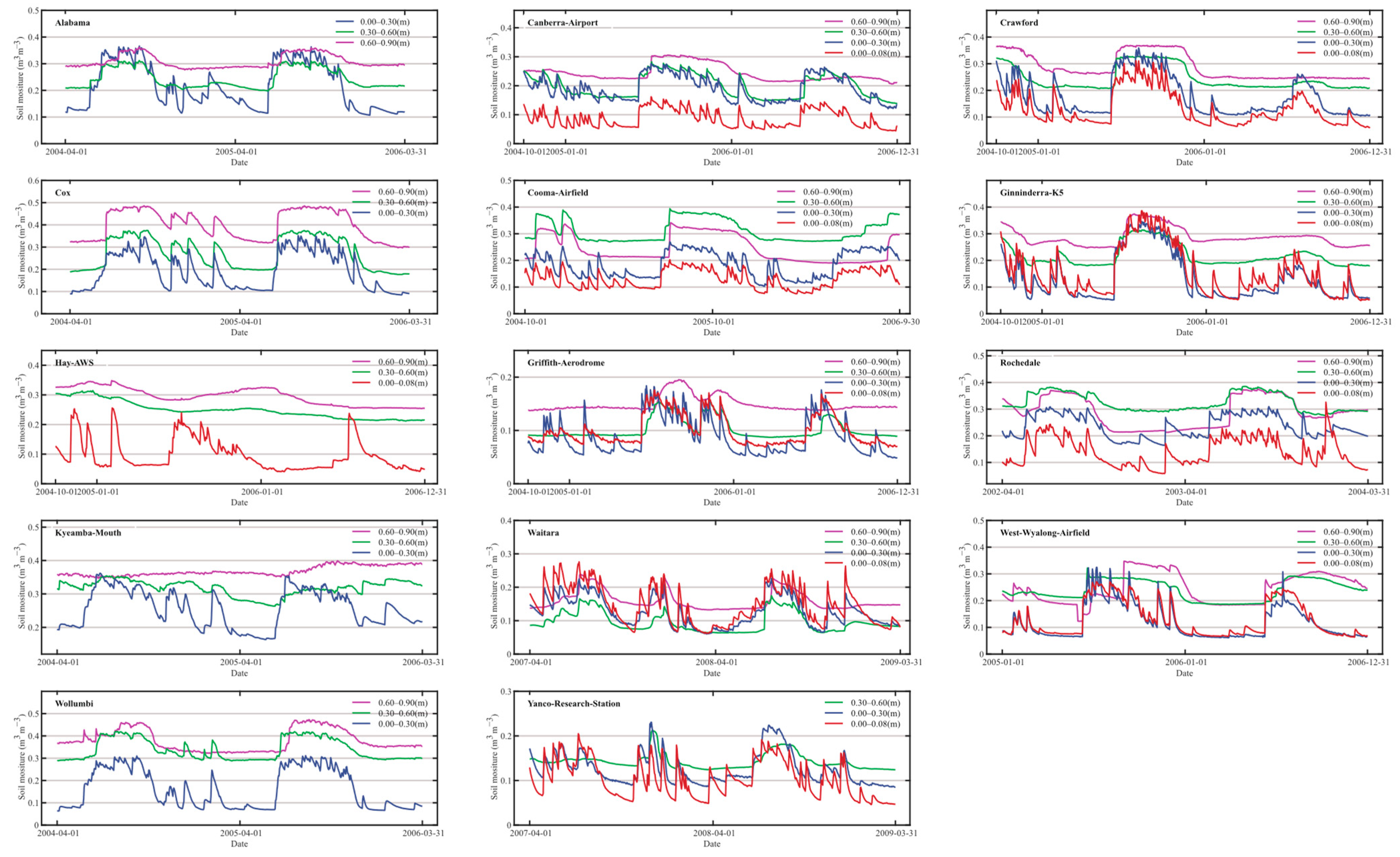
| Sites | 0–0.08 m | 0–0.3 m | 0.3–0.6 m | 0.6–0.9 m |
|---|---|---|---|---|
| Alabama | - | 47 | 50 | 55 |
| Canberra_Airport | 43 | 46 | 54 | 83 |
| Cooma_Airfield | 40 | 53 | 56 | 61 |
| Cox | - | 47 | 50 | 50 |
| Crawford | 54 | 54 | 64 | 77 |
| Ginninderra_K5 | 59 | 58 | 56 | 52 |
| Griffith_Aerodrome | 42 | 35 | 40 | 60 |
| Hay_AWS | 27 | - | 129 | 108 |
| Kyeamba_Mouth | - | 38 | 79 | 115 |
| Rochedale | 36 | 50 | 60 | 65 |
| Waitara | 26 | 59 | 61 | 65 |
| West_Wyalong_Airfield | 27 | 27 | 48 | 36 |
| Wollumbi | - | 51 | 51 | 58 |
| Yanco_Research_Station | 45 | 43 | 56 | - |
| All sites average | 40 | 47 | 61 | 68 |
| Type | ERA5-Land Layer 1 (0–7 cm) | GLDAS CLSM Surface (0–2 cm) | GLDAS NOAH (0–10 cm) | GLEAM v3.5a Surface (0–10 cm) | GLEAM v3.5b Surface (0–10 cm) | ESA CCI Soil Moisture (<2 cm) |
|---|---|---|---|---|---|---|
| Forest | 25.9 | 43.9 | 47.5 | 55.3 | 45.4 | 37.6 |
| Savanna | 20.9 | 41.0 | 39.7 | 41.9 | 36.7 | 31.6 |
| Shrubland | 15.8 | 37.2 | 27.4 | 37.5 | 31.2 | 32.6 |
| Agriculture | 29.2 | 55.1 | 48.1 | 59.8 | 51.7 | 38.4 |
| Grassland | 12.0 | 27.5 | 34.7 | 34.2 | 27.3 | 23.0 |
Publisher’s Note: MDPI stays neutral with regard to jurisdictional claims in published maps and institutional affiliations. |
© 2022 by the authors. Licensee MDPI, Basel, Switzerland. This article is an open access article distributed under the terms and conditions of the Creative Commons Attribution (CC BY) license (https://creativecommons.org/licenses/by/4.0/).
Share and Cite
Cai, J.; Chen, T.; Yan, Q.; Chen, X.; Guo, R. The Spatial-Temporal Characteristics of Soil Moisture and Its Persistence over Australia in the Last 20 Years. Water 2022, 14, 598. https://doi.org/10.3390/w14040598
Cai J, Chen T, Yan Q, Chen X, Guo R. The Spatial-Temporal Characteristics of Soil Moisture and Its Persistence over Australia in the Last 20 Years. Water. 2022; 14(4):598. https://doi.org/10.3390/w14040598
Chicago/Turabian StyleCai, Jiangtao, Tiexi Chen, Qingyun Yan, Xin Chen, and Renjie Guo. 2022. "The Spatial-Temporal Characteristics of Soil Moisture and Its Persistence over Australia in the Last 20 Years" Water 14, no. 4: 598. https://doi.org/10.3390/w14040598
APA StyleCai, J., Chen, T., Yan, Q., Chen, X., & Guo, R. (2022). The Spatial-Temporal Characteristics of Soil Moisture and Its Persistence over Australia in the Last 20 Years. Water, 14(4), 598. https://doi.org/10.3390/w14040598