1. Introduction
The ability to store water for electricity production, agriculture, or consumption is essential for modern societies. A fundamental prerequisite for water storage is safe dams. A failure of a dam may result in catastrophic consequences. Further, the construction and rehabilitation of dams have a high economic and environmental cost. These costs can be reduced if a dam’s operation without measures can be prolonged. To do so, with a maintained high level of safety, adequate assessments are required. Therefore, refined analyses and increased knowledge about the loads that act on dams facilitate prolonging their life span, resulting in substantial economic and environmental benefits.
Dams are mainly designed to withstand the loads caused by the impounded water. In addition to the pressure from the water, dams in cold regions may be exposed to loads from an ice sheet. This ice load is caused by the restrained expansion or movement of the ice and may constitute a significant fraction of the total horizontal loads. Current guidelines for ice load on dams are typically based on the geographical location of the dam but do not consider the local conditions [
1,
2,
3,
4,
5]. In these guidelines, the design ice load varies between 50 kN/m and 250 kN/m. Such magnitudes often cause a theoretically insufficient stability for load cases that includes ice loads in assessments of concrete dams in cold climate. However, the magnitude and return period of the ice loads are today among the most considerable uncertainty when evaluating dams in cold regions [
6]. Furthermore, there is a discrepancy between the number of dams where ice load is a theoretical problem, and the fact that few dam safety incidents have been reported where large ice loads has been identified as a cause.
There are four categories of methods for measuring the ice load on fixed structures: interfacial measurements, methods based on Newton’s second law, internal ice stress measurements, and structural response monitoring/hindcast calculations [
7]. A recent systematic literature review of ice load measurements on dams compiled 123 unique recordings of seasonal maximum ice loads [
8]. An overwhelming majority of these recordings are performed with local stress sensors or interfacial stress sensors that are considerably smaller than the dam–ice interaction area of interest. This difference leads to extrapolation and uncertainty regarding the representativeness of the measured local stresses, compared to the global structural load. One way to overcome this issue is by using the third measurement method, structural response monitoring (SRM). With this method, the ice loads are back-calculated from the measured response of the structure. SRM is the only ice load measurement method that determines the global load [
7]. The method is also relatively cheap to implement and use, only requires work performed on land above water, and the measurements can be used as a part of the dam owners continuous safety monitoring. Despite these advantages, only a few cases are reported where this method has been used for dams [
9,
10,
11,
12].
This study addresses this issue by back-calculating the ice load from observed displacement from dam safety monitoring of eight dam monoliths from five different dams. This is the first study to quantify the magnitude of ice loads on concrete dams based on their structural response. The back-calculated ice loads also add empirical data on the magnitude of global ice loads.
Section 2,
Section 3 and
Section 4 describe the methods and materials of this study. The two back-calculation approaches used to separate the displacement caused by ice loads from those caused by other loads are described in
Section 2, and
Section 3 describes the studied dams.
Section 4 presents the analysis methods and their application. These methods include finite element simulations of the ice–load–displacement relationship and the transient behavior of the dams, data-based models to predict the behavior of the dams and calculations of ice loads. The research findings are presented and discussed in
Section 5, focusing on three key themes: the expected structural response of the dams from ice loads, the accuracy of the applied methods and derived ice loads, and their practical implications. The conclusions from the research are summarized in
Section 6.
Table 1 explains the abbreviations that are used in figures and tables throughout the paper.
2. Back-Calculation of Ice Load
In the structural response monitoring method, the size of the ice load is back-calculated from the measured response of the structure. The method requires linearity between the ice load and the response [
7]. Provided that the behavior of the dam of interest is already monitored, back-calculation of the ice load is performed in three steps:
Estimation of the relationship between applied ice loads and displacements, i.e., the stiffness of the dam as a function of the ice load.
Separation of responses caused by ice loads from responses caused by other loads in the measured signal.
Calculation of the magnitudes of ice loads based on (1) and (2), respectively.
Assuming that the relationship between the ice load
I and the structural response
u is linear, the relationship between a change in load and response can be written as
where
is the structural stiffness with respect to the ice load. If the dam response to an ice load is established, for example, from simultaneous measurements of ice load and dam behavior, the stiffness can be calculated directly from the inverse of Equation (
1). If not, the stiffness can be estimated from a model
Here, is the model ice load, is the response, and is the estimated stiffness with respect to the ice load.
An observed change in the structural response,
, can be divided into three parts,
where
is the change caused by the ice load,
is the change caused by all other loads on the dam, and
is the observation error. Consequently, there are two main methods to estimate the size of the ice load from the measured signal. Either by using data where
so that Equation (
3) is reduced to
where
is an estimate of
, or by estimating
so that
From the estimated stiffness and the estimated measured response caused by the ice load, its magnitude can be estimated as
In this study, two methods have been used to quantify ; one event-based approach and one residual-based approach. These two methods are presented in the following sections.
2.1. Event-Based Approach
Ice load on dams occurs as events [
11,
13,
14,
15,
16,
17,
18,
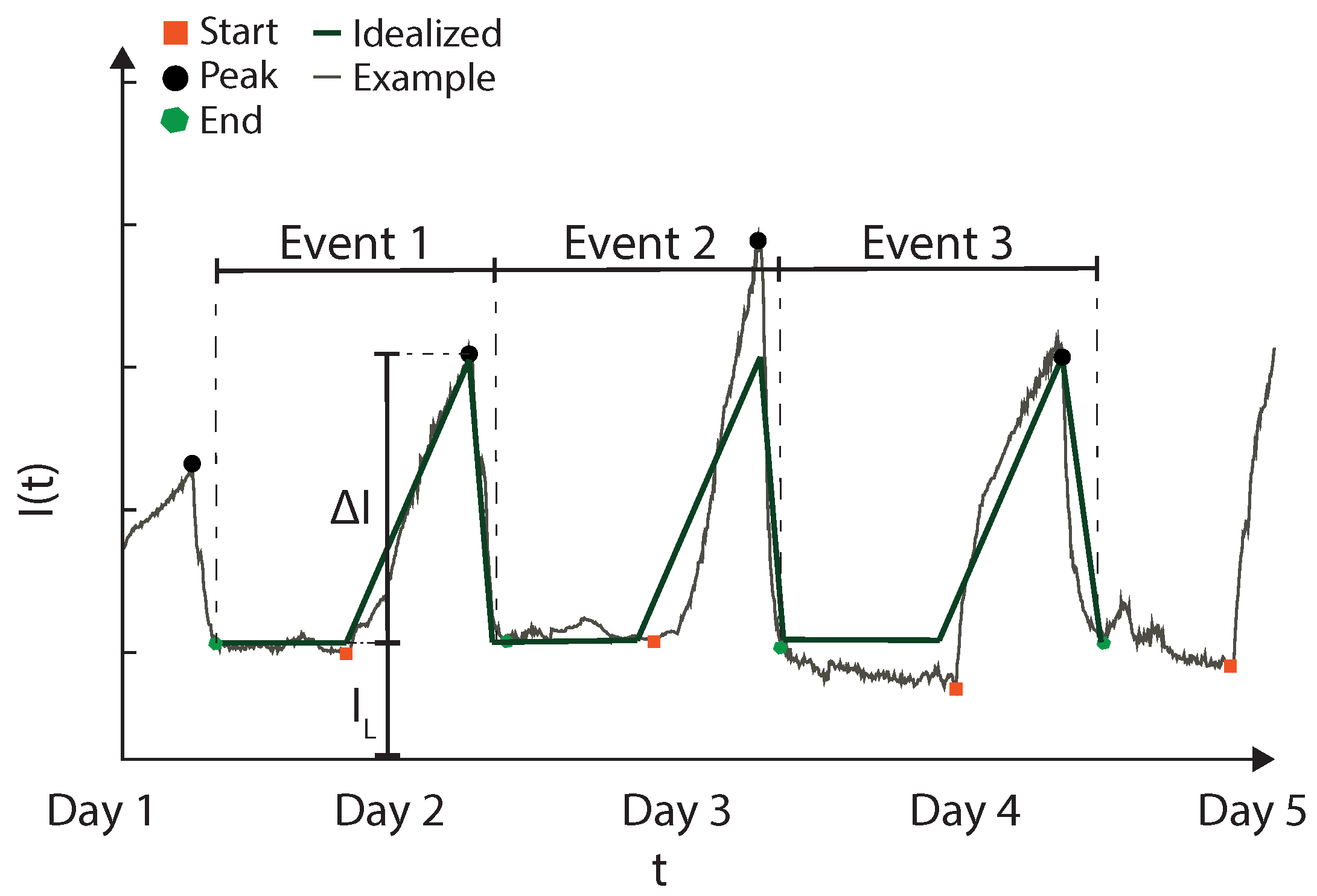
19], and such an event is characterized by
These ice load events predominantly last from hours up to a day, but can in some cases, last several days [
11].
Figure 1 shows examples of time-histories containing three ice load events, one idealized time-history from a design guideline [
20] and one measured time history, from Hellgren et al. [
21]. This event-shaped time history is caused by a combination of the loading mechanisms and the mechanical behavior of the ice. The main load-causing mechanisms for ice load on dams are restrained thermal expansions and water level fluctuations. These two mechanisms have short-term duration as the maximum variation is finite and can occur as a slow change over an extended period or a rapid change over a short period. Therefore, neither the temperature nor the water level can continuously increase or decrease for more than a limited period. The mechanical behavior of fresh-water ice is highly non-linear with a high initial creep rate. This creep relaxes the stress caused by the mechanism presented above so that the ice load continuously decreases during periods when no new load generating event occur.
With the first method, the ice load is back-calculated from events in the measured crest displacement. The ice load affects the dam behavior, and an ice load event causes the dam to deform in the downstream direction due to the increased load. By identifying displacement events in the measured signal, i.e., where the dam displaces from a local minimum to a peak, and if during such event, all displacements can be attributed to the ice load. The assumption that for dams during an ice load event as the duration of an event is insufficient for an ambient temperature change to affect the global behavior of the dam and that water level variations related to ice loads are relatively minor for the dam.
A displacement event can be identified in the dam monitoring signal as the difference between a local minimum and a maximum. By doing this for the entire signal,
N events can be identified.
After these events are identified, the maximum ice loads are estimated as follows:
The total ice load,
is the sum of a long-term ice load,
and an event ice load
, as
The long-term load describes the ice load at the start of the event and is a pressure built up in the ice over the winter. Comfort et. al. [
11] suggest that the long-term ice load
is a function of the ice thickness,
, and the ratio of the water level amplitude,
where
a is the average water level amplitude over two days. Equation (
10) provides the ice load in kN/m and is only valid for an ice thickness greater than 0.25 m and a ratio between
a and
greater than 0.08.
2.2. Residual-Based Approach
In the second method, the residual-based approach, a model is used to estimate the displacement of the dam caused by variation in all other factors except the ice load,
. For this, a model is used where
Here,
is the influence of hydrostatic pressure,
is the variation caused by changes in the ambient temperatures, and
is the irreversible changes that may occur over time. These three phenomena are the main causes of variation affecting the dam’s global behavior. After the displacement caused by the complementary loads to the ice load has been estimated, the signal from the dam monitoring can be adjusted by removing these effects.
For a model that perfectly describes the influence of
on the dam,
contains the effect from the ice load and the measurement errors. Consequently, the total ice load is estimated as
Figure 2 shows the difference between the two methods used to identify displacements caused by ice loads for a fictive displacement time-series.
3. Studied Dams
This study was performed as a case study where the ice load was back-calculated using measurement data from four concrete buttress dams: Bålforsen (BFN), Storfinnforsen (SFF), Ramsele (RSE), and Rätan (RTN), and one arch dam, Krokströmmen (KRN). From the four buttress dams, data from seven independent monoliths were included in the analysis, four from Storfinnforsen and one from each of the other dams. All dams are located in Sweden.
3.1. Dams
The five studied dams are all run-off-the-river plants, with small variations between the maximum and minimum allowable water levels in the reservoir (<0.5 m). All of these dams also have an insulation wall installed on the downstream side. These insulation walls reduces the displacements caused by seasonal temperature variations and thereby limits the risk of propagation of thermal cracks. For several of the buttress monoliths, the insulation wall was installed after the observation of through-cracks. The crack pattern for respective monolith includes several of the four crack types typically observed on buttress dams in Sweden: inclined cracks from the front plate that have propagated in the buttress toward the foundation, inclined cracks that have propagated from the inspection passage toward the front plate, and vertical cracks originating from the foundation, see [
22,
23].
The combination of small changes in water level and concrete temperature means that the dams are exposed to minimal external load changes other than the ice load. Therefore, these dam monoliths are suitable for back-calculations of the ice load.
Table 2 provides a summary of the included monoliths. Below, a short presentation of each studied dam is given.
3.1.1. Bålforsen
Bålforsen hydropower dam (BFN) is located in the river Umeälven in the northern region of Sweden and was constructed in 1958. In this study, data from concrete buttress monolith number 18 were used. The properties of the monolith are summarized in
Table 2 and a sketch of the section and the locations of sensors are shown in
Figure 3b. The data included from the dam are
the crest displacements measured with a hanging pendulum,
local displacements measured with five crack width sensors with a 220 mm center to center distance between anchorage points
the air temperature outdoors and in the enclosed area between the front plate and the insulation wall,
the water temperature at the depths of 3 and 17 m, and
water level.
3.1.2. Rätan
Rätan hydropower dam (RTN) in the river Ljungan, is a 31 m high concrete buttress dam constructed in 1968 and located 20 km north of the geographic midpoint of Sweden, in the northern ice load region. At Rätan, ice load measurements have been performed using a load panel between 2015–2021, see in [
19,
21]. Monolith 15, the monolith where the load panel is attached, is included in this study. The dimension of the monolith, its prominent cracks, and the position of the sensors are shown in
Figure 3a. The monolith is equipped with a hanging pendulum, that unfortunately is non-functioning. Instead, data from measurements of local displacements were used. The included data are
local displacements measured with two crack widths sensors with a 360 mm center to center distance between anchorage points;
the air temperature outdoors and in the enclosed area between the front plate and the insulation wall;
the water temperature at the depths of 3, 12, and 23 m; and
water level.
3.1.3. Krokströmmen
Krokströmmen hydropower dam (KRN) is located in the river Ljusnan, 30 km south of the geographical midpoint of Sweden and in the northern ice load region. The concrete dam is an arch dam that was constructed in 1952. The properties of the dam are presented in
Table 2 and the section of monolith 10 are shown in
Figure 3h. The included data are
the crest displacements measured with a hanging pendulum located at monolith 10,
the air temperature outdoors,
the water temperature at the depths of 3 and 20 m, and
water level.
This data from the external variables are available with hourly frequency from December 2016. However, the logging of the pendulum was non-functioning from November 2017. Thereby, only approximately one year of crest displacement recordings are available.
3.1.4. Ramsele and Storfinnforsen
Ramsele (RSE) and Storfinnforsen (SFF) are two concrete buttress dams built in the 1950s, located 10 km apart in the Faxälven river in the the northern ice load region of Sweden. The Storfinnforsen concrete dam consists of 81 independent concrete buttress monoliths, of which four are equipped with hanging pendulums. The monoliths are, Monolith 03 (
Figure 3c), Monolith 42 (
Figure 3d), Monolith 43 (
Figure 3e), and Monolith 46 (
Figure 3f), referred to as M03, M42, M43, and M46, respectively. The concrete dam at Ramsele consists of 49 independent monoliths, where the tallest monoliths are slightly higher than 40 m. From Ramsele dam, data from Monolith 23 (
Figure 3g) was included in this study.
Both of these dams have recently undergone extensive renovation and rehabilitation measures, which includes a new monitoring program and installation of post-tensioned rock-anchored tendons through the buttress wall to increase stability. New sensors have been continuously added after the start of the new program in 2019. Therefore, the availability of data from secondary measurement such as indoor temperatures and water temperatures vary but are overall sparse. The data included from the dam are
the crest displacements measured with a hanging pendulums,
the air temperature outdoors, and
water level.
4. Analysis Methods
The eight monoliths were studied in two types of analyses: a pre-study that investigates the influence of previously measured ice loads on the transient behavior of the dams under normal conditions, and estimating the ice loads these dams have been subjected to from their measured structural response. The following analyzes were performed:
Pre-study
Estimation of ice loads
Table 2 presents the performed analysis for each dam. A more detailed presentation of each analysis is given in the following sections.
4.1. Finite Element Analyses
Three different FE-analyses were performed: one simulation of the transient behavior of the dam without ice load (1-I); one simulation of the transient behavior with applied ice load (1-II); and one to estimate the stiffness, i.e., the ice load–displacement relationship (2-I). All numerical analyses were performed with Abaqus [
24], version 2021, using the standard implicit solver. The models used for the simulations includes the dam and part of the surrounding rock. All models are reused from the previous studies, and a more thoughtful description of the FE-models are given in the respective studies, see
Table 3 for sources. The dams were modeled in 3D with 8-node linear brick elements with reduced integration and hourglass control (DC3D8 and C3D8R in Abaqus) or 6-node linear triangular prism elements (DC3D6 and C3D8 in Abaqus), see
Table 3. A maximum element size of 0.3 m. was used for the dams. The elements of the rock match the dams at the interface surface with increasing size towards the outer edge of the models. In the mechanical model, the boundary conditions were applied to the rock by prohibiting displacements perpendicular to each side at all outer boundaries of the rock, except the top surface. The interaction properties for the interface between dam and foundation, and a linear elastic constitutive model were used for all materials with properties chosen according to previous studies as presented in
Table 3 for each dam, respectively.
All different simulations were all performed in three steps. In the first step, the gravity load was applied to the dam. In the second step, the hydrostatic pressure corresponding to the maximum water level was applied on the upstream part of the rock and dam. The third step differed between the three analyses. In analyses 1-I and 1-II, the transient behavior of the dams was simulated with and without ice load. These simulations were performed in two domains, for temperature and mechanical equilibrium. In the temperature model, an adiabatic boundary condition was applied to all rock surfaces except the top surface. The top of the rock and the dam was divided into four categories of surfaces: outside, indoor, insulation, and water. On each surface, the corresponding measured temperature was applied using robin boundary condition. All temperatures are shown in
Figure 4. Time steps of different length was used between periods with and without expected ice load. A two week time step was used for the period May to December and a six hour time time step for the period where ice loads are expected (January to April). The resulting temperature field was used as input to the mechanical model with a one-way coupling. Therefore, the resulting temperature distribution from the thermal domain was applied in the mechanical domain, and the strains and corresponding displacements from temperature variation were calculated using the same time steps.
In analysis 1-II, the transient simulation with ice load, the magnitude of the measured ice loads from [
19,
21] was applied as a uniform pressure on a one-meter high surface under the maximum water level. These data were used for all included dams. The data contain measurements from six winters. However, the signal is only complete from ice formation to ice break up for four of these winters, 2016/2017, 2018/2019, 2019/2020, and 2020/2021. Therefore, the recordings from these winters where used recurringly in that order to cover the period from 2012–2021.
Figure 4 shows the applied ice load and
Table 2 presents an overview of the performed analysis and used data.
In analysis 2-I, the ice load was applied the same one-meter high surface as in analysis 1-II in 30 kPa (30 kN/m) steps up to 300 kPa (300 kN/m). To mimic the measurement data, displacements corresponding to the measured were extracted from the simulated deformations of the dam. From these displacements, a relation between the magnitude of the ice load and the measured deformation of the dam was calculated.
4.2. Data-Based Models
Data-based models were used to back-calculate the ice load with the residual approach. These models where used to create adjusted measurement series, i.e., a measuring series where the effect from all external loads (except the ice loads) were removed. There are many types of data-based models intended to predict the behavior of dams [
31]. In general, data-based models have a better prediction accuracy than FE-models, but are less interpretable. For this reason, two data-based models with a distinct physical coupling were chosen. The model are hydrostatic temperature and time (HTT) and hydrostatic seasonal time (HST). In the following section, a description of the implementation of these models is given.
4.2.1. Hydrostatic, Seasonal, Time Model
The HST model was first introduced in [
32] and has thereafter been used as a method for behavior analysis of several types of dams [
33,
34,
35,
36,
37,
38,
39,
40]. HST is a multilinear regression model, where the variation in behavior of a dam is assumed to be function of three parts:
H, the influence of hydrostatic pressure;
S, seasonal effects; and
t, time-dependent effects. The model thus includes a function for each phenomenon considered to affect the global behavior of the dam and is based on the hypothesis that these three variables are sufficient to explain the variation in behavior. Furthermore, the three variables are also assumed to be independent of each other.
The response of the dam can thus be written as
In the literature, the hydrostatic pressure is predominantly modeled with a third- or fourth-degree polynomial. However, the dams in this case study all are exposed only to small water level variations. Therefore, a simple linear relation can be assumed [
41],
where
h is the relative water level related to the dam height
and the reservoir level,
, according to
where
is the bottom level.
Figure 4 shows
h for all dams.
In HST, the seasonal variation with the first terms in a periodic Fourier series, according to
where
L = 52.18 if the time variable
t has the unit of weeks. This type of function assumes that the behavior of the dam follows a seasonal pattern consisting of a full-year period and a half-year period.
The last effect is the irreversible changes over time. In this study, a linear relationship is assumed for this effect,
4.2.2. Hydrostatic, Thermal, Time Model
With the HTT model, the seasonal behavior is replaced by a function that considers the actual temperature,
In this study, the outside air temperature
, indoor air temperature
, and water temperature
from each dam was used.
The HTT model was not used for Storfinnforsen and Ramsele as the required input data is unavailable. For the arch dam at Krokströmmen, was omitted. For those dams with several thermometers at different water depths, the temperatures recorded by the topmost thermometers were included in the data-based analysis.
4.2.3. Data Preparation
From the monitoring, two type of recordings were included in this study. The first type is global measurements of the crest displacement by hanging pendulums. In this study, positive changes correspond to a movement of the crest in the downstream direction, i.e., the direction the crest displaces from an increase in ice load. The included data all have a frequency of one sample per hour. The second type of included of measurements are local displacements, recorded with crack width sensors. The data from such sensors were combined through a dimension reduction using a principal component analysis (PCA), and the first principal component (PC1) was used in the analyses. The PCA was performed on the simulated response to the ice load and results in a linear combination of the crack width signal that maximize the response caused by ice loads in the recorded signals.
For fitting of the data-based models, the temperatures and response signals were re-sampled to a time-step of two weeks. In the re-sampling, the actual measured value was used and no aggregation for the data between time steps were performed. The models were fitted on the complete time-series of re-sampled data, thus without a division into training and test set. After the fitting of each model, the residuals was calculated using the actual frequency of the recorded signals.
4.3. Time History and Event Identification
Ice load events were identified via a search to find local maxima and minima in the recorded signals, i.e., the time history of the pendulum and PC1 data. A local maximum or minimum was defined as an extreme value during at least 6 h. After identifying a peak in the signal, an iteration was performed to find the nearest previous and immediate following local minimum. These three points were used to define ice load events with time and magnitude for the start, peak, and end, respectively. This search was performed with the find_peaks function from the Signal subpackage of the SciPy package [
42].
4.4. Calculation of Ice Load
For all dams, the ice load was estimated using the event-based approach. From the identified events in crest displacements and PC1, all differences between the minimum value at the start of the event and the peak were assumed to be caused by the ice load. For the event-based approach, the ice thickness is a required input to Equation (
10). In this study, the ice thickness was estimated using Stefans equation where the ice thickness,
, is calculated from the accumulated freezing degree days (AFDD)
where
is a coefficient to account for local conditions. In this study,
was used, recommended for conditions that maximize the ice thickness, i.e., a windy lake with no snow cover [
43].
For the monoliths with a data period longer than two years the ice load was also calculated with the residual approach, see
Table 2. In the residual approach, all positive residuals during the winter were interpreted as an ice load.
5. Result and Discussion
This section presents and discuss the results from the case studies and the back-calculation of ice loads. It starts with a comparison of the measured dam behavior and the predicted behavior from the three model types. After that, the estimated ice load–displacement relation is presented for each dam and behavior before the identified, and back-calculated ice load events and residual ice loads are shown.
5.1. Stiffness
Figure 5 shows the calculated crest displacement as function of ice load and presents the calculated stiffness. The relationship between increased ice load and the crest displacement and is linear for all dams. The magnitude of ice load required to displace the crest 1 mm ranges between 86 kN/m for the arch dam at Krokströmmen and 254 kN/m for Bålforsen. The monoliths at Storfinnforsen and Ramsele all have similar stiffness where an ice load of approximately 160 kN/m is required to displace the dam crest 1 mm. This indicates that the load–displacement relationship is relatively constant for dams of this type. The slope of this relationship is similar also for all seven buttress monoliths, despite their different heights and shapes. If any, the results show a small negative relation between the stiffness and the dam height.
The ice load–displacement relationship is linear also for the two PC1 signals. The slope of these relationships does not have an interpretable unit, as the data was standardized before the PCA. For Rätan, the components are 0.59 and 0.80 for sensors 1 and 2, respectively. For Bålforsen, the other dam with local sensors, the weights in PC1 are −0.16, 0.82, 0.43, 0.08, and 0.35 for Sensors 1–5, respectively. Therefore, the sensors best positioned to capture effects from the ice load are sensors 2, followed by sensors 3 and 5. Sensor 2 and 3 are located orthogonal and parallel to the crack running vertically from the inspection gallery to the foundation, while Sensor 5 are located on the front plate.
5.2. Time History of Displacements
Figure 6 shows the measured and modeled time history from the three model types—HST, HTT, and FEM—for the crest displacement and PC1 of local displacements.
Figure 6 shows that the ice load of the magnitude measured and applied in this project are large enough to be detected visually in the measured crest displacement. This difference is highlighted for Rätan dam as shown in
Figure 6a, where only the results from analyses 1-I and 1-II, the simulations with and without ice loads, are presented. However, this effect can also be seen for Bålforsen in
Figure 6b. For Krokströmmen, the only arch dam, the ice load creates increased variation in the crest movements during the winter, but the magnitudes of these variations are relatively small and not necessarily distinguishable from the noise in the signal. One possible explanation for this difference is that the ice load does not act in the downstream direction along the whole arch dam. Thus, the dam displacements from increased ice loads are not fully represented by the downstream crest displacements measured by the pendulum. Another possible explanation is the lesser insulation and lack of heating that causes larger natural crest variations for Krokströmmen compared to the other dams. Therefore, the influence from the ice load is relatively smaller and more difficult to distinguish from the influence of other loads. This difference between the displacements for simulations with and without ice loads can also be seen in the PC1 signals from Rätan in
Figure 6g, but is not as prominent as for the crest displacements.
5.3. Accuracy
Table 4 presents the root mean square error (RMSE) and the coefficient of determination (R
) for analyses 1-I, 2-II-ii-A, and 2-II-ii-B. The RMSE provides an absolute measure of fit in the units mm and kN/m, which is easier to interpret but only relevant for internal comparison. In contrast, the R
is a relative measure of fit that can be used in comparisons between dams. All FEM models capture the expected direction of the measured displacements well but do, for some periods, predict the incorrect magnitude of the variations. The two comparisons between simulated and measured crest displacements score R
values of 0.76. However, the two models differ significantly in the RMSE. For the FE model of Krokströmmen, where the RMSE for the displacement is 3.44 mm, and the stiffness (86 kN/m/mm), the RMSE corresponds to an ice load of 296 kN/m. Such magnitudes of errors make it impossible to accurately back-calculate the ice load using the residual-based approach. For the FE model of Bålströmmen, the mean error is smaller but still considerable. The FEM model of Rätan shows an adequate ability to capture the local response of the dam while the FE-model of Bålforsen shows an insufficient ability to capture the local response of the dam. For that reason, the accuracy of the derived stiffness is uncertain, and the PC1 from Bålforsen was therefore excluded from further analyses.
For both approaches, potential sources of error include the measuring accuracy of the dam monitoring equipment and estimation of the load–displacement relationship. Good quality and accuracy of the measurements are essential for the quantification of the influence of different loads in the response of a dam. The installed pendulums have an accuracy of 0.01 mm [
44] which translates to ice loads of approximately 0.8–2.5 kN/m based on the stiffness presented in
Section 5.1. The error on the estimated ice load is directly proportional to the error of the estimated stiffness. For the crack width sensors, the accuracy is 0.005 mm and the resolution 0.00125 mm [
45]. The observed variation between winter and summer for the crack with sensors with the largest variation is approximately 0.4 mm. Thus, the relative accuracy is lower for the crack width sensor than for the pendulum. This can be observed in the time history where the crest displacement signal is more smooth than the PC1 signal. The lack of resolution means that the PC1 signal varies between two discrete levels during some periods. This variation is sometimes incorrectly classified as events, which could have been avoided with higher resolution.
In the residual approach, the assumption is that the models can be used to remove the influence from all loads except the ice load from the measured signal. The model with the best prediction accuracy in this study was HTT. This model was used in the residual approach to create an adjusted signal where effects from temperature, water level, and time were removed. The HST provides R
values in the range 0.7–0.9, while R
for the HTT is over 0.89 in all comparisons. Thus, the linear combination of temperatures, water level, and time that is HTT can explain over 90% of the variance in displacements. These results can be compared to the work in [
40] where a HST model was used on the buttress dams at Ancipa (R
= 0.95–0.97), Sabbione (R
= 0.95–0.96), and Malga Bissina (R
= 0.88–0.91, 0.92, 0.92, 0.90), and the results from in [
39] where crest the crest displacement of a buttress dam was predicted with HST (R
= 0.95) and HTT (R
= 0.96). Thus, the prediction accuracy for the models in this study is similar to previous studies. However, the result presented in
Table 4 shows that despite the high accuracy of the data-based models, the RMSE as ice load is relatively large. For the four predictions of crest displacements, the RMSE is between 27 and 57 kN/m. Furthermore, as shown in
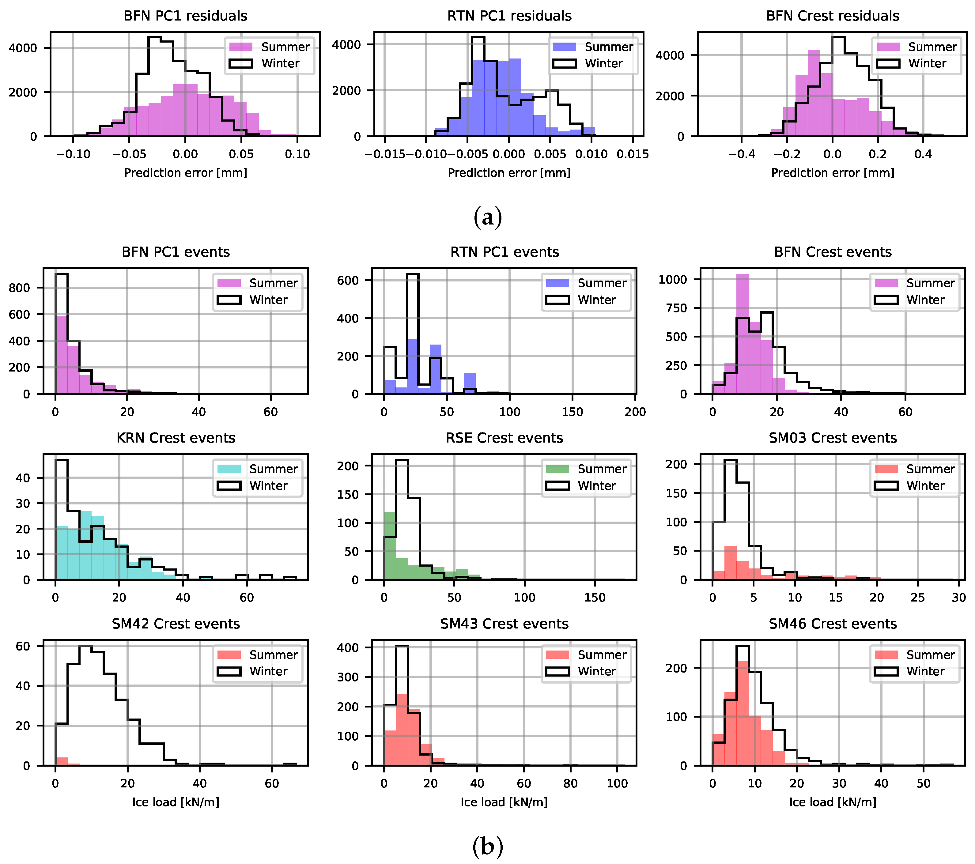
Figure 7, the errors are similarly distributed during both summer and winter, with only a slight tendency for the average errors to be greater during the winter. Furthermore, the most significant errors and ice loads are similarly frequent during summer and winter. Thus, the accuracy of the ice loads calculated with the residual approach was deemed unreliable. Therefore, only the ice loads from the event-based approach were included as the final results.
5.4. Time History of Ice Loads
Figure 8 shows a time history of the total ice load calculated with the event-based approach for both crest displacement and the first PC1 of the crack width sensors. The figure shows two main results: that the calculated ice loads are small and and that the deviation in crest displacement during periods with expected ice loads are similar to those from the rest of the year. In general, the ice loads are low and are combined for all dams other than Rätan, only a few occasions of ice loads in the vicinity of 100 kN/m. In comparison with the expected response of the dams shown in
Figure 6, the ice loads and underlying displacements are small.
Figure 8 also shows that events occur during all months and that the most prominent occur during periods with no ice in the reservoir.
Figure 7b show histograms of the identified ice load events during summer and winter. For a dam exposed to significant ice loads, the expected result is that both events will be greater and more frequent during January to April when ice loads are expected to occur. Such a trend is not visible neither in the events nor in the residuals or the resulting ice loads. A t-test for difference in the means of the events’ magnitude between winter and summer shows that the upper limit of the 95% confidence interval for the difference is from −2.2 kN/m for SM03 to 4.2 kN/m for Bålforsen, where a positive value means a larger mean for the winter period. There are two implications of these results:
The first implication is a problem for the accuracy of the method and the estimated loads. Several improvements could be made to the classification algorithms, such as filtering the signal based on frequency or applying post-peak criteria. However, this study applied a conservative approach to ensure that the ice loads were not underestimated. In the event-based approach, all displacements that occur during an event was assumed to be caused by ice loads. During a thermal ice load event, the air temperature increases and warms the downstream part of the dam. When the temperature in this downstream part increases, thermal expansion causes a crest displacement in the upstream direction. Such displacement is in the opposite direction to a displacement caused by ice loads and could thereby conceal the influence from this load. However, the high thermal mass of concrete results in slow thermal expansion. During an event caused by water level variation, the hydrostatic pressure will also vary from the changed water level. However, this difference is also negligible as any significant water level change will break the ice sheet.
The presence of ice loads of similar magnitude and frequency during winter and summer implies that several of the events inferred as ice loads should be attributed to noise in the measured signal. Therefore, the magnitude of ice loads presented in this study is most likely overestimated. Furthermore, the static equilibrium requires the dam the deform in response to the ice load. The absence of clear evidence of such responses are a indication that the dams have not been subjected to any major global ice loads.
5.5. Annual Max of Ice Loads
Table 5 presents the maximum total ice load from each winter (Jan–April) for all included monoliths. This table shows the results without considering the reservations discussed above. The results can be divided into three categories: The first category is the single winter from the arch dam at Krokströmmen, where the maximum magnitude was 83 kN/m. The second category is the 20 winters from the remaining buttress dams. For these dams, the data from the crest displacement measurements indicate that the maximum ice load event for a typical winter is between 50 and 100 kN/m, with two occurrences of ice loads over 100 kN/m.
The third category is the eight winters of PC1-data from Rätan. During these winters, the estimated ice loads are between 67 and 205 kN/m. For seven of the eight winters, the maximum estimated ice load exceeds 100 kN/m. The results from Rätan Dam can be compared with ice loads measured with a load panel on the upstream face of the dam [
19,
21]. The measured ice loads with the load panel are presented in
Figure 8. During the six seasons of measurements, the 1 m wide and 3 m high load panel recorded 73 ice load events with a magnitude greater than 75 kN/m and an overall maximum of 200 kN/m. During the eight winters in this study, which includes the six winters with measurements, the maximum ice load estimated from the response of the dam is 205 kN/m and 52 events greater than 75 kN/m was identified. Only two of the events occur simultaneously, i.e., ice loads were registered both by the panel and in the dam’s response. These two events occurred on 5 and 19 February 2020. On the first occasion, an ice load of 111 kN/m was measured with the panel, while the estimated total ice load from the dam’s response was 77 kN/m. The corresponding loads for the second occasion are 99 and 78 kN/m.
Traditionally, the ice load has been measured with a sensor in the ice or on the dam face. Previous measurements campaigns with such sensors have recorded ice load with significantly larger magnitudes than the design loads and those estimated in this study, e.g., 780 kN/m from one season at the Beaumont dam [
46], 600 kN/m from one winter with four stress cell panels at the La Gabelle dam [
46], 370 kN/m from five winters at Seven sisters dam [
11], 290 kN/m from four winters at the Eleven Mile Canyon dam [
47], 270 kN/m from five winters with three to four panels at the Tradalsvik dam [
48], 200 kN/m from one winter with eleven panels at the Barrett Chute dam [
49], and 200 kN/m for six winters with the load panel, and 720 kN/m from one winter with three stress cell panels at the Rätan dam [
19].
One possible explanation for the small ice loads estimated in this study is scale effects, i.e., that local ice loads on a small area can be significantly larger than the mean of the global ice loads on the whole structure. This phenomenon is considered in design standards for piers, off-shore structures, and ships [
20,
50,
51], but not in design guidelines for dams [
1,
2,
3,
4,
5]. Ice is a material whose behavior and strength are scale-dependent. A compilation of 2073 freshwater ice beam tests shows that the scale-dependent flexural strength in kPa is proportional to
[
52], where
V is the volume of the beam. For ice–structure interaction, the same general relation also applies, and the average ice load decreases as the area of interaction increases. The relationship between volume and the flexural strength for freshwater ice presented in [
52] gives that flexural strength for an ice volume with the width of 8 m (a dam monolith) is 7% of that of a 1 m wide volume (the load panel). The results from this study indicate that the scale effect is applicable also for dam–ice interaction and that further studies is needed to investigate how the ice loads vary along the dam and between different scales.
5.6. Practical Implications
The Swedish guidelines for ice loads on bridge piers and dams are essentially the same recommendations as given in the first guidelines from 1931 [
53]. The foreword to the latest revision of the recommendations for ice loads on bridges in Sweden states that these first ice loads recommendations were created based on no actual knowledge but has gained empirical validation [
54]. There are simultaneous indications that the ice loads in design guidelines are either over- or underestimated. The results from previous existing measurements and the theoretical models indicate that the current guidelines underestimate the magnitudes of ice loads. However, a common result in assessments of concrete dams in cold regions is insufficient stability for load cases that includes ice loads. For this reason, several Swedish dams has been rebuilt or strengthen to ensure sufficient stability. Despite this, there is a general public opinion among dam engineers that the current guidelines are too strict. The use of these design magnitudes worldwide in design of dams for almost a century has resulted in few incidents and no failures reported as induced by ice loads.
For the design of concrete dams, the relevant load is the global ice load, i.e., the average load on the width of the structure. This ice load is not a load in the pure sense but rather a restraint force where the ice load is the restrained movement or expansion of the ice sheet. A dam subjected to ice loads will deform until a new equilibrium position is reached. Ice loads of the magnitude in current design guidelines constitute a significant portion of the the total horizontal load on most dams. These ice loads’ magnitude combined with the long lever arm from the foundations theoretically causes a large structural response. This large expected influence of ice loads is also shown in the results from analyses 1 (I and II) and 2-II in this study.
The most probable interpretation of the results of this study is that no or very small traces of ice load can be observed in the measured response of most dams. These results are limited to the eight studied dam monoliths. However, as the ice load was included as a design load for dams approximately hundred years ago without any theoretical basis, ice loads has not caused any major incidents. Therefore, a main focus of future investigation should be to find full-scale empirical evidence of existence of global ice loads on dams of a relevant magnitude. It is likely that such evidence can be found, but before this, it is recommended that studies are performed to investigate that ice loads on concrete dams can pose a dam safety issue.
Such investigations should primarily focus on finding influence of ice loads in the structural behaviour of concrete dams. Using measurements from the dam monitoring to estimate the magnitude of the ice load is a cost-effective method that has advantages from both a scientific and dam safety perspective. From a scientific perspective, this type of measurement provides a cheap method that is readily accessible for many dams. The method also facilitates the use of data already collected, as long as it was sampled with a sufficiently high frequency. Therefore, the method presents an opportunity to rapidly expand the empirical data on the impact of ice loads on concrete dams. From a dam safety perspective, the installation of a global displacement sensor such as a hanging pendulum have several benefits. For dams where the dam owner wants to examine or monitor the magnitude of the ice load, such a method is therefore very advantageous.
6. Conclusions
This study estimates the magnitude of the ice load on an arch dam and seven monoliths from four concrete buttress dams, based on measured structural response during 29 winters. The main results are the magnitudes of ice loads calculated using identified displacement events in the measured signals. With this event-based approach, the loads were estimated from identified displacement events in the measured signal and interpreted as ice loads using a displacement–ice load relationship derived from FE simulations. The results from the FE simulations show that ice loads of magnitudes from traditional ice load measurement sensors and the applicable design guideline should significantly affect the studied dam structural response and be detected by traditional dam monitoring. Nevertheless, only small traces of ice loads can be found in the observed response of the studied dams.
The annual maximum magnitudes of ice loads estimated in this study are significantly smaller than those recorded during ice loads measurements sensors and in design guidelines. However, the results show that displacement events occur with similar frequencies and magnitudes during all months. Therefore, the conservative assumption used in this study, that ice loads cause all displacements during events, is likely to cause an overestimation of the ice loads. Therefore, the event-based approach applied in this study provides a conservative estimate of the magnitude. The true magnitude of the ice loads these dams have been subjected to is most likely even lower.
This study involves modeling the structural behavior of several concrete dams located in cold climates. Therefore, some auxiliary conclusions regarding the interpretation and modeling of the behavior of the dams in this study, adjacent to the primary research question for this study, are:
The relationship between increased ice load and crest displacements in the downstream direction is linear up to 300 kN/m/mm. For the seven studied buttress monoliths, the slope of the ice load–displacement relationship is approximately 180 kN/m/mm, while the corresponding slope for the arch dam is 90 kN/m/mm.
The magnitudes of ice loads recorded with traditional ice load measurement sensors and the applicable design guideline should cause structural displacements that are visible in the measured crest displacements of dams. The influence from ice loads should be especially prominent in such recordings from dams in reservoirs with small water level fluctuations and where the natural thermal variations between winter and summer have been dampened by insulation and heating.
The HTT model that considers a linear combination of variations in water level, ambient temperatures, and time can explain over 90% of the variance in the dams’ displacements.
The insulation walls on the downstream part of the dam monoliths and the heating of the enclosed area between the front plate and the insulation have a significant influence on the behavior of the dam. These measures both reduce the magnitude and change the phase and shape of the variation in displacements from air and water temperature variation.
This study demonstrates the need to further investigate the relationship between stresses measured in the ice sheet, pressures measured at the dam–ice interaction face, and the dam’s response. Further research should be undertaken to investigate the influence of ice loads on the structural behavior of concrete dams. The event-based method used in this study is fast and straightforward and, therefore, suitable for applying on other dams. Such studies could rapidly increase the empirical knowledge regarding the magnitudes of ice loads on dams.
Author Contributions
Conceptualization, R.H. and R.M.; methodology, R.H.; software, R.H.; validation, R.H.; formal analysis, R.H.; investigation, R.H.; resources, R.M. and A.A.; data curation, R.H.; writing—original draft preparation, R.H.; writing—review and editing, R.M., J.E., A.A. and E.N.; visualization, R.H.; supervision, R.M., A.A. and E.N.; project administration, R.M.; funding acquisition, R.M. All authors have read and agreed to the published version of the manuscript.
Funding
This research received no external funding.
Institutional Review Board Statement
Not applicable.
Informed Consent Statement
Not applicable.
Data Availability Statement
Not applicable.
Acknowledgments
The research presented was carried out as a part of “Swedish Hydropower Centre—SVC”. SVC has been established by the Swedish Energy Agency, Energiforsk and Svenska Kraftnät together with Luleå University of Technology, KTH Royal Institute of Technology, Chalmers University of Technology and Uppsala University (
www.svc.nu accessed on 7 February 2022).
Conflicts of Interest
The authors declare no conflict of interest.
References
- RIDAS. Swedish Hydropower Companies Guidelines for Dam Safety, Application Guideline 7.3 Concrete Dams; Technical Report; Swedenergy: Stockholm, Sweden, 2021. [Google Scholar]
- NVE. Retningslinje for Laster og Dimensjonering [Guideline for Loads and Dimensioning]; Technical Report; NVE: Oslo, Norway, 2003. [Google Scholar]
- FERC. Engineering Guidelines for the Evaluation of Hydropower Projects: CHAPTER III Gravity Dams; Technical Report; Federal Energy Regulatory Commission: Washington, DC, USA, 2016.
- Alberta Transportation. Water Control Structures, Selected Design Guidlines; Technical Report; Transportation and Civil Engineering Division: Calgary, AB, Canada, 2004. [Google Scholar]
- CFBR. Recommandations Titre du Colloque Pour la Justification de la Stabilité des Barrages Poids [Recommendations for the Justification of the Stability of Gravity Dams]; Technical Report; Comité Français des Barrages et Réservoirs (CFBR) qui: Paris, France, 2012. [Google Scholar]
- Westberg Wilde, M.; Johansson, F. Probabilistic Model Code for Concrete Dams; Technical Report; Energiforsk: Stockholm, Sweden, 2016. [Google Scholar]
- Bjerkås, M. Review of Measured Full Scale Ice Loads to Fixed Structures. In Proceedings of the 26th International Conference on Offshore Mechanics and Arctic Engineering, San Diego, CA, USA, 10–15 June 2007; pp. 1–10. [Google Scholar] [CrossRef]
- Hellgren, R.; Malm, R. A Systematic Literature Search and Meta Regression of Measured Ice Load on Dams; KTH Royal Institute of Technology: Stockholm, Sweden, 2021. [Google Scholar]
- Zhang, M.; Qu, X.; Kalhori, H.; Ye, L. Indirect monitoring of distributed ice loads on a steel gate in a cold region. Cold Reg. Sci. Technol. 2018, 151, 267–287. [Google Scholar] [CrossRef]
- Zhang, M.; Qiu, B.; Kalhori, H.; Qu, X. Hybrid reconstruction method for indirect monitoring of an ice load of a steel gate in a cold region. Cold Reg. Sci. Technol. 2019, 162, 19–34. [Google Scholar] [CrossRef]
- Comfort, G.; Gong, Y.; Singh, S.; Abdelnour, R. Static ice loads on dams. Can. J. Civ. Eng. 2003, 30, 42–68. [Google Scholar] [CrossRef]
- Hellgren, R.; Malm, R.; Persson, A.; Klasson Svensson, E. Estimating the effect of ice load on a concrete dams displacement with regression models. In Proceedings of the ICOLD 2017 International Symposium, Knowledgebased Dam Engineering, Prague, Czech Republic, 3–7 July 2017; International Commission on Large Dams: Prague, Czech Republic, 2017. [Google Scholar]
- Carter, D.; Sodhi, D.; Stander, E.; Caron, O.; Quach, T. Ice thrust in reservoirs. J. Cold Reg. Eng. 1998, 12, 169–183. [Google Scholar] [CrossRef]
- Stander, E. Ice Stresses in Reservoirs: Effect of Water Level Fluctuations. J. Cold Reg. Eng. 2006, 20, 52–67. [Google Scholar] [CrossRef]
- Taras, A.; Côté, A.; Comfort, G.; Thériault, L.; Morse, B. Measurements of Ice Thrust at Arnprior and Barrett Chute Dams. In Proceedings of the 16th Workshop on the Hydraulics of Ice Covered Rivers, Winnipeg, MB, Canada, 18–22 September 2011; pp. 317–328. [Google Scholar]
- Côté, A.; Taras1, A.; Comfort, G.; Morse, B. Static ice loads at dam face and at far field. In Proceedings of the 23rd IAHR International Symposium on Ice, Ann Arbor, MI, USA, 31 May–3 June 2016; pp. 1–8. [Google Scholar]
- Petrich, C.; Sæther, I.; Fransson, L.; Sand, B.; Arntsen, B. Time-dependent spatial distribution of thermal stresses in the ice cover of a small reservoir. Cold Reg. Sci. Technol. 2015, 120, 35–44. [Google Scholar] [CrossRef] [Green Version]
- Foss, A.B. Islast Mot Dammer Med Varierende Vannstand [Ice Loads on Dams with Water Level Variation]. Master’s Thesis, Norwegian University of Science and Technology, Trondheim, Norway, 2017. [Google Scholar]
- Hellgren, R.; Petrich, C.; Arntsen, B.; Malm, R. Ice load measurements on Rätan concrete dam using different sensor types. Cold Reg. Sci. Technol. 2022, 193, 103425. [Google Scholar] [CrossRef]
- ISO-19906; ISO-19906:2010: Arctic Offshore Structures. Technical Report; Petroleum and Natural Gas Industries: Geneva, Switzerland, 2010.
- Hellgren, R.; Malm, R.; Fransson, L.; Johansson, F.; Nordström, E.; Westberg Wilde, M. Measurement of ice pressure on a concrete dam with a prototype ice load panel. Cold Reg. Sci. Technol. 2020, 170, 102923. [Google Scholar] [CrossRef]
- Malm, R.; Gasch, T.; Eriksson, D. Evaluating stability failure modes due to cracks in a concrete buttress dam. In Proceedings of the ICOLD 2013 International Symposium; International Commission on Large Dams (ICOLD): Seattle, WA, USA, 2013; pp. 1–10. [Google Scholar]
- Malm, R.; Ansell, A. Cracking of Concrete Buttress Dam Due to Seasonal Temperature Variation. ACI Struct. J. 2011, 108, 13–22. [Google Scholar]
- Dassault Systemes. Abaqus CAE (Version 2021); Dassault Systemes: Vélizy-Villacoublay, France, 2021. [Google Scholar]
- Hellgren, R.; Malm, R.; Nordström, E. Modeller för öVervakning av Betongdammar [Models for Monitoring of Concrete Dams]; Technical Report; Energiforsk: Stockholm, Sweden, 2019. [Google Scholar]
- Hellgren, R.; Malm, R.; Ansell, A. Performance of data-based models for early detection of damage in concrete dams. Struct. Infrastruct. Eng. 2020, 17, 1–15. [Google Scholar] [CrossRef]
- Andersson, O.; Seppälä, M. Verification of the Response of a Concrete Arch Dam Subjected to Seasonal Temperature Variations. Master’s Thesis, KTH Royal Institute of Technology, Stockholm, Sweden, 2015. [Google Scholar]
- Malm, R.; Broberg, L.; Enzell, J.; Blomdahl, J.; Nilsson, C.O. Predicting the measured behaviour and defining warning levels of a concrete dam. In Proceedings of the 27th ICOLD Congress, Marseille, France, 27 May–3 June 2021; International Commission on Large Dams (ICOLD): Marseille, France, 2021. [Google Scholar]
- Malm, R.; Nordström, E.; Nilsson, C.O.; Tornberg, R.; Blomdahl, J. Analysis of potential failure modes and re- instrumentation of a concrete dam. In Proceedings of the ICOLD Symposium—Appropriate Technology to Ensure Proper Development, Operation and Maintenance of Dams in Developing Countries, 84th ICOLD Meeting in Johannesburg, Johannesburg, South Africa, 15–20 May 2016; pp. 1–11. [Google Scholar]
- Hellgren, R.; Malm, R. A parametric numerical study of factors influencing the thermal ice pressure along a dam. In Proceedings of the 25 IAHR International Symposium on Ice, Trondheim, Norway, 23–25 November 2020; pp. 823–832. [Google Scholar]
- Salazar, F.; Morán, R.; Toledo, M.; Oñate, E. Data-Based Models for the Prediction of Dam Behaviour: A Review and Some Methodological Considerations. Arch. Comput. Methods Eng. 2017, 24, 1–21. [Google Scholar] [CrossRef] [Green Version]
- Willm, G.; Beaujoint, N. Les méthodes de surveillance des barrages au service de la production hydraulique d’Èlectricité De France. In Proceedings of the IXth International Congress on Large Dams, Vienna, Austria, 4–6 July 2018; International Commission on Large Dams (ICOLD): Istanbul, Turkey, 1967; pp. 529–550. [Google Scholar]
- Chouinard, L.E.; Bennett, D.W.; Feknous, N. Statistical Analysis of Monitoring Data for Concrete Arch Dams. J. Perform. Construct. Facil. 1995, 9, 286–301. [Google Scholar] [CrossRef]
- Dufour, F.; Tatin, M.; Briffaut, M.; Simon, A.; Fabre, J.P.P. Thermal displacements of concrete dams: Accounting for water temperature in statistical models. In Proceedings of the Second International Dam World Conference, Lisbon, Portugal, 21–24 April 2015; pp. 1–9. [Google Scholar] [CrossRef]
- Tatin, M.; Briffau, M.; Dufour, F.; Simon, A.; Fabre, J.P.P.; Briffaut, M.; Dufour, F.; Simon, A.; Fabre, J.P.P. Statistical modelling of thermal displacements for concrete dams: Influence of water temperature profile and dam thickness profile. Eng. Struct. 2018, 165, 63–75. [Google Scholar] [CrossRef]
- Dai, B.; Gu, C.; Zhao, E.; Qin, X. Statistical model optimized random forest regression model for concrete dam deformation monitoring. Struct. Control Health Monit. 2018, 25, e2170. [Google Scholar] [CrossRef]
- Fabre, J.P.; Hueber, R. Exploitation of Monitoring Result to Adapt the Operation of Dams to Their Behaviour. In Proceedings of the Long Term Behaviour of Dams, Graz, Austria, 12–13 October 2009; pp. 347–352. [Google Scholar]
- Zou, J.; Bui, K.T.T.; Xiao, Y.; Doan, C.V. Dam deformation analysis based on BPNN merging models. Geo-Spat. Inf. Sci. 2018, 21, 149–157. [Google Scholar] [CrossRef] [Green Version]
- Nedushan, B.A. Multivariate Statistical Analysis of Monitoring Data for Concrete Dams. Ph.D. Thesis, McGill University, Montreal, QC, Canada, 2002. [Google Scholar]
- De Sortis, A.; Paoliani, P. Statistical analysis and structural identification in concrete dam monitoring. Eng. Struct. 2007, 29, 110–120. [Google Scholar] [CrossRef]
- Hellgren, R. Condition Assessment of Concrete Dams in Cold Climate. Ph.D. Thesis, KTH Royal Institute of Technology, Stockholm, Sweden, 2019. [Google Scholar]
- Virtanen, P.; Gommers, R.; Oliphant, T.E.; Haberland, M.; Reddy, T.; Cournapeau, D.; Burovski, E.; Peterson, P.; Weckesser, W.; Bright, J.; et al. SciPy 1.0: Fundamental Algorithms for Scientific Computing in Python. Nat. Methods 2020, 17, 261–272. [Google Scholar] [CrossRef] [Green Version]
- USACE. Engineering and Design: Ice Engineering; Technical Report; US Army Corps of Enginners: Washington, DC, USA, 2006.
- Geokon. Pendulum Readout: Model 6850; Technical Report; Geokon: Lebanon, PA, USA, 2015. [Google Scholar]
- Geosense. VW Crack Meter VWCM-4000; Geosense Ltd.: Bury Saint Edmunds, UK, 2019. [Google Scholar]
- Bisanswa, D. Poussée de Glaces en 2009 sur les Barrages de la Rivière St-Maurice. Master’s Thesis, Université Laval, Quebec City, QC, Canada, 2011. [Google Scholar]
- Monfore, G.E. Ice pressure: Experimental investigations by the bureau of reclamation. Trans. Am. Soc. Civ. Eng. 1954, 119, 26–38. [Google Scholar] [CrossRef]
- Petrich, C.; Sæther, I.; Sadnick, M.O.; Arntsen, B. Static ice loads on a dam in a small Norwegian reservoir. In Proceedings of the 25 IAHR International Symposium on Ice, Trondheim, Norway, 23–25 November 2020; pp. 23–25. [Google Scholar]
- Côté, A.; Taras, A.; Comfort, G.; Morse, B. Hydro Quebec ice load measurement program. In Proceedings of the 2012 CDA Annual Conference on Dam Safety, Saskatoon, SK, Canada, 22–27 September 2012; Canadian Dam Association: Saskatoon, SK, Canada, 2012; pp. 1–12. [Google Scholar]
- Swedish Maritime Services. Finnish-Swedish Ice Class Rules: The Structural Design and Engine Output Required of Ship for Navigation in Ice; Technical Report; Swedish Maritime Administration: Norrköping, Sweden, 2014.
- CAN/CSA. CAN/CSA S472-92: Foundations; Technical Report; Canadian Standards Association: Toronto, ON, Canada, 1992. [Google Scholar]
- Aly, M.; Taylor, R.; Bailey Dudley, E.; Turnbull, I. Scale Effect in Ice Flexural Strength. J. Offshore Mech. Arct. Eng. 2019, 141. [Google Scholar] [CrossRef]
- SOI. SOI 1931:30 Normalbestämmelser för Järnkonstruktioner till Byggnadsverk [Design Manual for Steel Structures]; Technical Report; Statens Offentliga Utredningar: Stockholm, Sweden, 1931.
- Vägverket. Istryck mot bropelare [Ice Pressure on Bridge Piers]; Technical Report; Vägverket: Stockholm, Sweden, 1987. [Google Scholar]
Figure 1.
Illustration of ice load events with an idealized and real case. The idealized case is after ISO-19906 [
20] and the example from Hellgren et al. [
21].
Figure 1.
Illustration of ice load events with an idealized and real case. The idealized case is after ISO-19906 [
20] and the example from Hellgren et al. [
21].
Figure 2.
Illustration of the two methods used to identify displacements caused by ice loads in the observed displacements.
Figure 2.
Illustration of the two methods used to identify displacements caused by ice loads in the observed displacements.
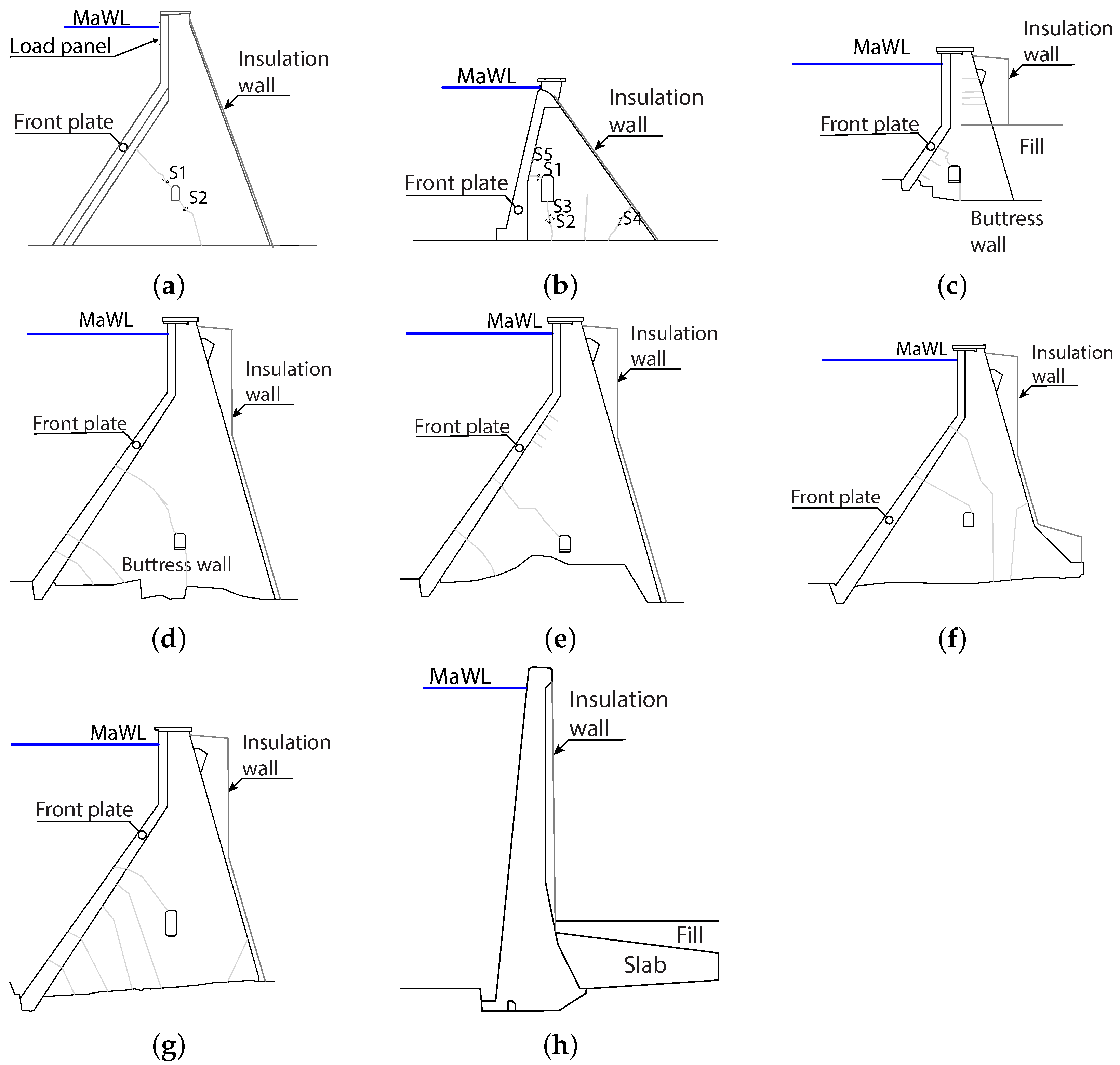
Figure 3.
Dam sections for the monoliths used in the case study. The light gray line shows a sketch of the location of the cracks included in the simulation, and the dark gray shows the insulations walls. (
a) RTN, (
b) BFN, (
c) SM03, (
d) SM42, (
e) SM44, (
f) SM46, (
g) RSE, (
h) KRN. MaWL: Maximum retention water level, the abbreviations for the dam names are presented in
Table 2.
Figure 4.
Input data for the analysis.
Figure 4.
Input data for the analysis.
Figure 5.
Ice load–displacement relationship. The legend presents the slope for each line in the kN/m per displacement unit. (a) Crest displacement, (b) PC1 of local displacements.
Figure 5.
Ice load–displacement relationship. The legend presents the slope for each line in the kN/m per displacement unit. (a) Crest displacement, (b) PC1 of local displacements.
Figure 6.
Measured and modeled time history for the eight included dams: crest displacements; (a) RTN, (b) BFN, (c) SM03, (d) SM42, (e) SM44, (f) SM03, (g) RSE, (h) KRN; and the first principal component of the crack width measurements; (j) BFN and (i) RTN.
Figure 6.
Measured and modeled time history for the eight included dams: crest displacements; (a) RTN, (b) BFN, (c) SM03, (d) SM42, (e) SM44, (f) SM03, (g) RSE, (h) KRN; and the first principal component of the crack width measurements; (j) BFN and (i) RTN.
Figure 7.
Distribution of events and residuals and during the summer (June to September) and ice load season (January to April). (a) Residuals. (b) Events. For visibility, have 15 events from BFN-PC1 with magnitudes over 50 kN/m and 4 events from RTN-PC1 with magnitudes over 200 kN/m been removed. None of the removed events occurred during a winter.
Figure 8.
Time history of the total ice load (event + long-term) identified and back-calculated from events in the crest displacements and the first principal component of the crack width sensors. (a) RTN, (b) BFN, (c) KRN, (d) SM03, (e) SM42, (f) SM44, (g) SM03, (h) RSE.
Figure 8.
Time history of the total ice load (event + long-term) identified and back-calculated from events in the crest displacements and the first principal component of the crack width sensors. (a) RTN, (b) BFN, (c) KRN, (d) SM03, (e) SM42, (f) SM44, (g) SM03, (h) RSE.
Table 1.
Abbreviations used in the paper.
Table 1.
Abbreviations used in the paper.
| Abbverition | Full Name |
|---|
| AFDD | Accumulated freeze degree days |
| BFN | Bålforsen dam |
| Crest | Crest displacments |
| FEM | Finite element model |
| HTT | Hydrostatic, Thermal, Time model |
| HST | Hydrostatic, Seasonal, Time model |
| KRN | Krokströmmen dam |
| PCA | Principal component analysis |
| PC1 | First principal component |
| RSE | Ramsele dam |
| RMSE | Root mean square error |
| RTN | Rätan dam |
| R | Coefficient of determination |
| SFF | Storfinnforsen dam |
| WLA | Water level amplitude |
Table 2.
Overview of basic characteristics, the data and the performed analysis for each dam.
Table 2.
Overview of basic characteristics, the data and the performed analysis for each dam.
| | Type | Buttress | Arch |
|---|
| | Dam | Rätan | Bålforsen | Storfinnforsen | Ramsele | Krokströmmen |
|---|
| | Name | RTN | BFN | SM03 | SM42 | SM43 | SM46 | RSE | KRN |
|---|
| Info | Monolith | 15 | 18 | - | 3 | 42 | 43 | 46 | 23 |
| | Length [m] | 9.0 | 8.0 | 8.0 | 8.0 | 8.0 | 8.0 | 8.0 | 160 |
| | Height [m] | 31.0 | 20.75 | 18.0 | 41.0 | 39.0 | 36.0 | 37.0 | 45.0 |
| Data | Start * | 13/10 | 12/12 | 19/11 | 20/10 | 19/02 | 19/02 | 19/07 | 16/12 |
| | End * | 21/05 | 21/05 | 21/06 | 21/06 | 21/06 | 21/06 | 21/02 | 17/11 |
| | Crest | - | X | X | X | X | X | X | X |
| | Crack width | X | X | - | - | - | - | - | - |
| | | X | X | X | X | X | X | X | X |
| | | X | X | - | - | - | - | - | - |
| | | X | X | - | - | - | - | - | X |
| | WL | X | X | X | X | X | X | X | X |
| | Ice load | X | † | † | † | † | † | † | † |
| Analysis | 1-I | X | X | - | - | - | - | - | X |
| | 1-II | X | X | - | - | - | - | - | X |
| | 2-I | X | X | X | X | X | X | X | X |
| | 2-II-i | X | X | X | X | X | X | X | X |
| | 2-II-ii-A | X | X | - | - | - | X | X | - |
| | 2-II-ii-B | X | X | - | - | - | - | - | - |
Table 3.
Material properties used for simulations of the different dams.
Table 3.
Material properties used for simulations of the different dams.
| | | Unit | BFN | KRN | SFF | RSE | RTN |
|---|
| Concrete | Density | kg/3 | 2300 | 2700 | 2300 | 2300 | 2300 |
| | Elastic modulus | GPa | 21.7 | 30 | 25.0 | 25.0 | 30.0 |
| | Poisson’s ratio | - | 0.2 | 0.2 | 0.2 | 0.2 | 0.2 |
| | Conductivity | W/ | 1.7 | 1.7 | - | - | 1.7 |
| | Specific heat | J/K | 1000 | 1000 | - | - | 1000 |
| | Expansion | 1/K | 10.6 | 10.0 | - | - | 10.6 |
| | Element type | - | Brick | Tet | Brick | Brick | Brick |
| Rock | Density | kg/3 | 2300 | 2500 | 2300 | 2300 | 2300 |
| | Elastic modulus | GPa | 32.0 | 50.0 | 60.0 | 60.0 | 50.0 |
| | Poisson’s ratio | - | 0.2 | 0.2 | 0.2 | 0.2 | 0.2 |
| | Conductivity | W/ | 1.7 | 1.7 | 1.8 | 1.8 | 1.7 |
| | Specific heat | J/K | 1000 | 1000 | - | - | 1000 |
| | Expansion | 1/K | 8.3 | 8.0 | - | - | 10.0 |
| | Element type | - | Brick | Tet | Tet | Tet | Brick |
| Temp-BC | Reference temperature | C | 4 | 0 | - | - | 4 |
| | filmCoeff water | /2/ | 500 | 500 | - | - | 500 |
| | filmCoeff air | /2/ | 13 | 13 | - | - | 13 |
| | filmCoeff insulation | /2/ | 1 | 1 | - | - | 1 |
| | Dam-Rock interaction | - | Tie | Tie | Fric | Fric | Fric |
| | Friction coefficient | - | - | - | 1.0 | 1.0 | 1.0 |
| | Source | | [25,26] | [27] | [28,29] | [28,29] | [30] |
Table 4.
The root mean squared error (RMSE) and R for the three analyses for crest displacement and PC1.
Table 4.
The root mean squared error (RMSE) and R for the three analyses for crest displacement and PC1.
| | | | Crest | PC1 |
|---|
| | | | 1-I | 2-II-ii-A | 2-II-ii-B | 1-I | 2-II-ii-A | 2-II-ii-B |
|---|
| Dam | Type | Unit | FEM | HST | HTT | FEM | HST | HTT |
|---|
| BFN | R | - | 0.76 | 0.70 | 0.89 | 0.06 | 0.78 | 0.94 |
| | RMSE | mm | 0.21 | 0.23 | 0.13 | 0.13 | 0.06 | 0.03 |
| | † | kN/m | 52 | 57 | 33 | 467 | 222 | 112 |
| KRN | R | - | 0.76 | - | - | - | - | - |
| | RMSE | mm | 3.44 | - | - | - | - | - |
| | † | kN/m | 295 | - | - | - | - | - |
| RTN | R | - | - | - | - | 0.81 | 0.97 | 0.97 |
| | RMSE | mm | - | - | - | 0.01 | 0.005 | 0.004 |
| | † | kN/m | - | - | - | 352 | 146 | 130 |
| SM43 | R | - | - | 0.92 | - | - | - | - |
| | RMSE | mm | - | 0.16 | - | - | - | - |
| | † | kN/m | - | 27 | - | - | - | - |
| SM46 | R | - | - | 0.78 | - | - | - | - |
| | RMSE | mm | - | 0.24 | - | - | - | - |
| | † | kN/m | - | 39 | - | - | - | - |
Table 5.
The annual maximum of total ice load, event ice load, long-term ice load, ice thickness, accumulated degree freeze days (AFFD), the minimum temperature, and the mean water level amplitude. Note that the time of the different extreme values for the different variables during a winter does not necessarily occur simultaneously.
| | | Ice Load | Ice Thick. | Temp. | AFDD | WLA |
|---|
| Dam | Winter | Total | Event | Long-Term | | min | | Mean |
|---|
| | | kN/m | m | C | C Days | m/Day |
|---|
| BFN * | 2013 † | 97 | 75 | 30 | 0.75 | −25 | 772 | 0.20 |
| | 2014 | 60 | 43 | 21 | 0.48 | −26 | 321 | 0.24 |
| | 2015 | 65 | 54 | 18 | 0.48 | −23 | 316 | 0.23 |
| | 2016 | 73 | 53 | 27 | 0.65 | −27 | 579 | 0.19 |
| | 2017 | 64 | 54 | 14 | 0.54 | −25 | 401 | 0.24 |
| | 2018 | 58 | 37 | 31 | 0.78 | −25 | 835 | 0.24 |
| | 2019 | 87 | 67 | 29 | 0.73 | −27 | 728 | 0.23 |
| | 2020 | 61 | 51 | 22 | 0.50 | −21 | 348 | 0.18 |
| | 2021 | 52 | 30 | 26 | 0.62 | −24 | 524 | 0.10 |
| KRN | 2017 † | 84 | 75 | 13 | 0.46 | −25 | 287 | 0.17 |
| RSE | 2020 | 107 | 89 | 20 | 0.46 | −19 | 285 | 0.06 |
| | 2021 | 59 | 38 | 30 | 0.72 | −26 | 704 | 0.05 |
| RTN | 2014 † | 68 | 64 | 9 | 0.37 | −17 | 186 | 0.16 |
| | 2015 | 115 | 99 | 18 | 0.54 | −20 | 403 | 0.14 |
| | 2016 | 208 | 182 | 28 | 0.69 | −24 | 646 | 0.16 |
| | 2017 | 173 | 155 | 20 | 0.54 | −19 | 405 | 0.15 |
| | 2018 | 152 | 130 | 33 | 0.81 | −24 | 898 | 0.15 |
| | 2019 | 116 | 97 | 27 | 0.65 | −21 | 576 | 0.16 |
| | 2020 | 101 | 91 | 15 | 0.43 | −13 | 251 | 0.15 |
| | 2021 | 118 | 117 | 27 | 0.65 | −23 | 572 | 0.12 |
| SM03 | 2020 | 33 | 13 | 20 | 0.46 | −19 | 286 | 0.05 |
| | 2021 | 46 | 18 | 30 | 0.71 | −26 | 701 | 0.04 |
| SM42 | 2021 | 95 | 67 | 30 | 0.71 | −26 | 701 | 0.04 |
| SM43 | 2019 | 49 | 24 | 26 | 0.60 | −21 | 502 | 0.05 |
| | 2020 | 71 | 57 | 20 | 0.46 | −19 | 286 | 0.05 |
| | 2021 | 108 | 79 | 30 | 0.71 | −26 | 701 | 0.04 |
| SM46 | 2019 | 76 | 53 | 26 | 0.60 | −21 | 502 | 0.05 |
| | 2020 | 66 | 51 | 20 | 0.46 | −19 | 286 | 0.05 |
| | 2021 | 87 | 57 | 30 | 0.71 | −26 | 701 | 0.04 |
| Publisher’s Note: MDPI stays neutral with regard to jurisdictional claims in published maps and institutional affiliations. |
© 2022 by the authors. Licensee MDPI, Basel, Switzerland. This article is an open access article distributed under the terms and conditions of the Creative Commons Attribution (CC BY) license (https://creativecommons.org/licenses/by/4.0/).


