
Detecting the Planform Changes Due to the Seasonal Flow Fluctuation and 2012 Severe Flood in the Amazon River near Iquitos City, Peru Based on Remote Sensing Image Analysis


Abstract
:1. Introduction
2. The Upper Peruvian Amazonian Rivers
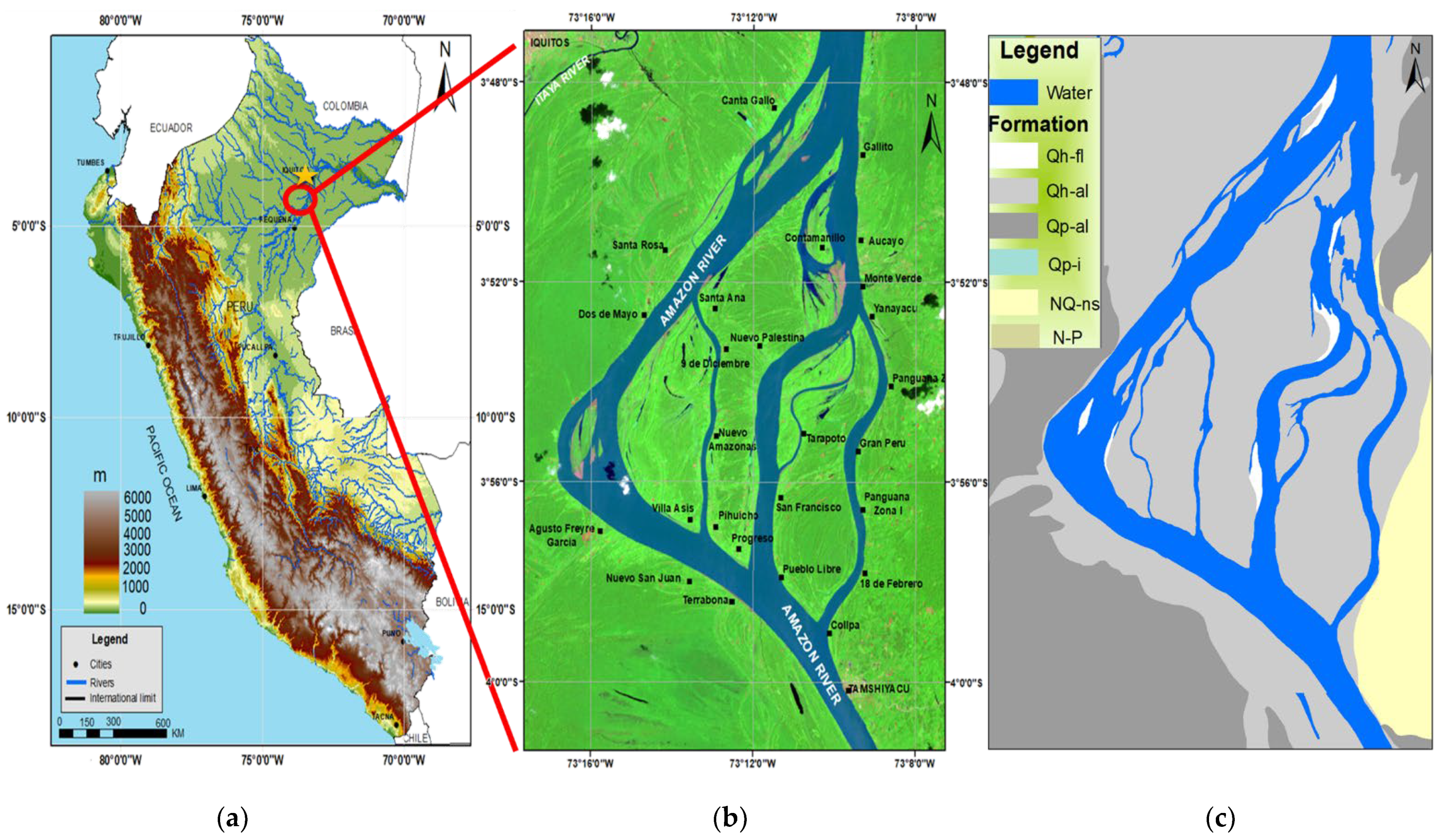
3. Study Area
3.1. Description of the Muyuy Anabranching Structure
3.2. Geologic Background
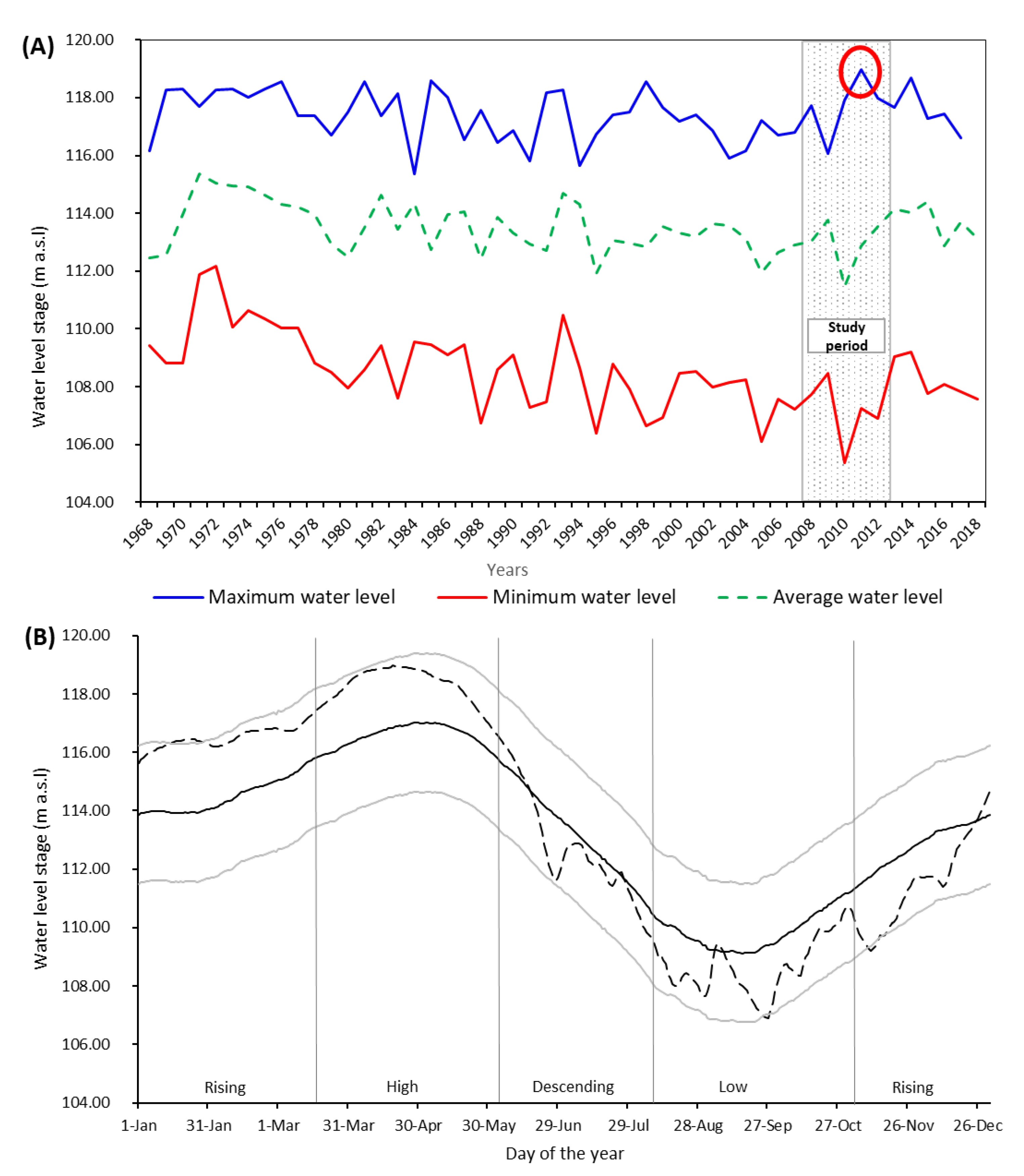
3.3. Water Level Variations of the Amazon River
3.4. Dynamics of Muyuy Anabranching Structure
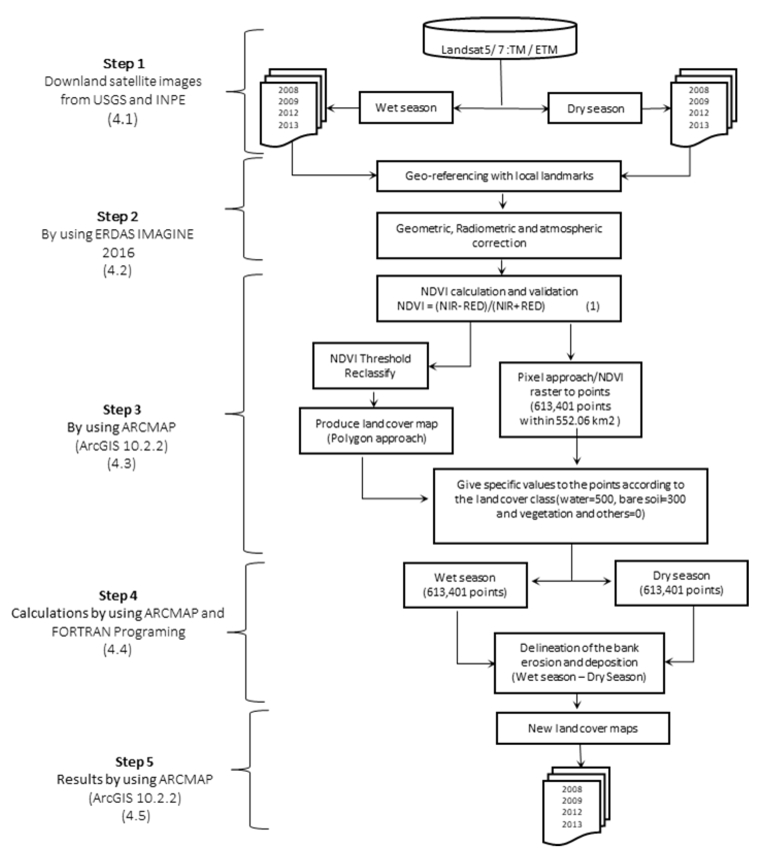
4. Methodology
4.1. Planform Change Detection Based on Image Classification (Step 1)
4.2. Images Processing (Step 2)
4.3. NDVI Calculation and Validation (Step 3)
4.4. Land Cover Classification Based on NDVI (Step 4)
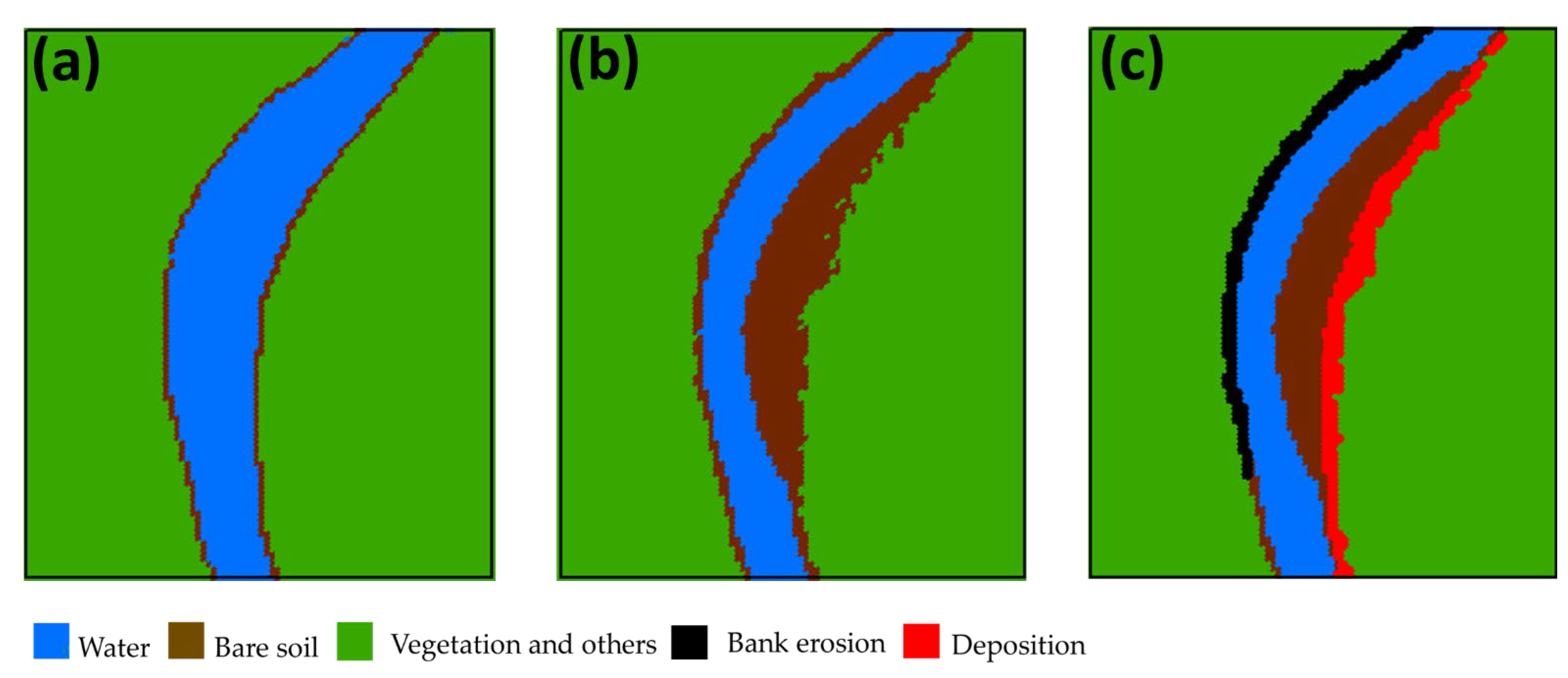
4.5. Delineation of Bank Erosion and Deposition (Step 5)
5. Results and Discussion
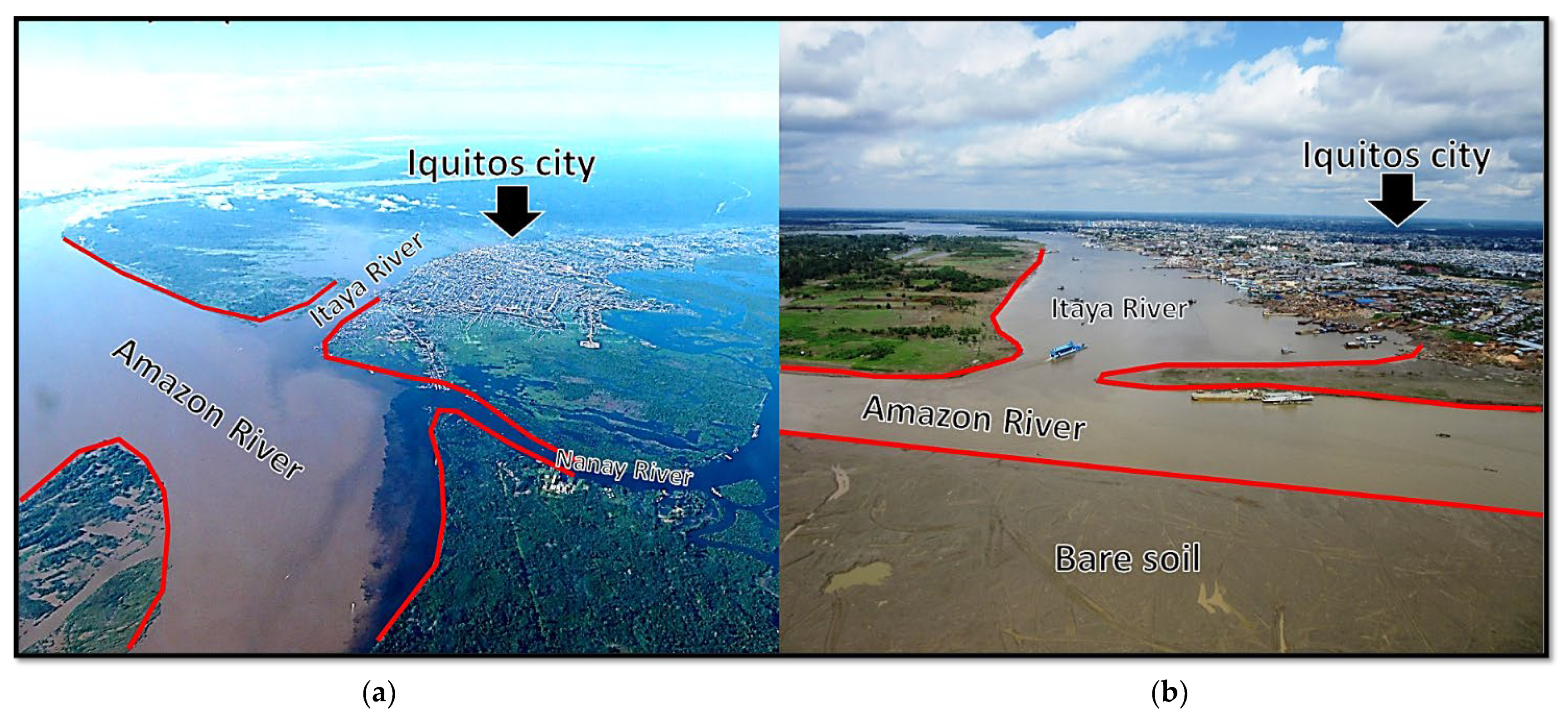
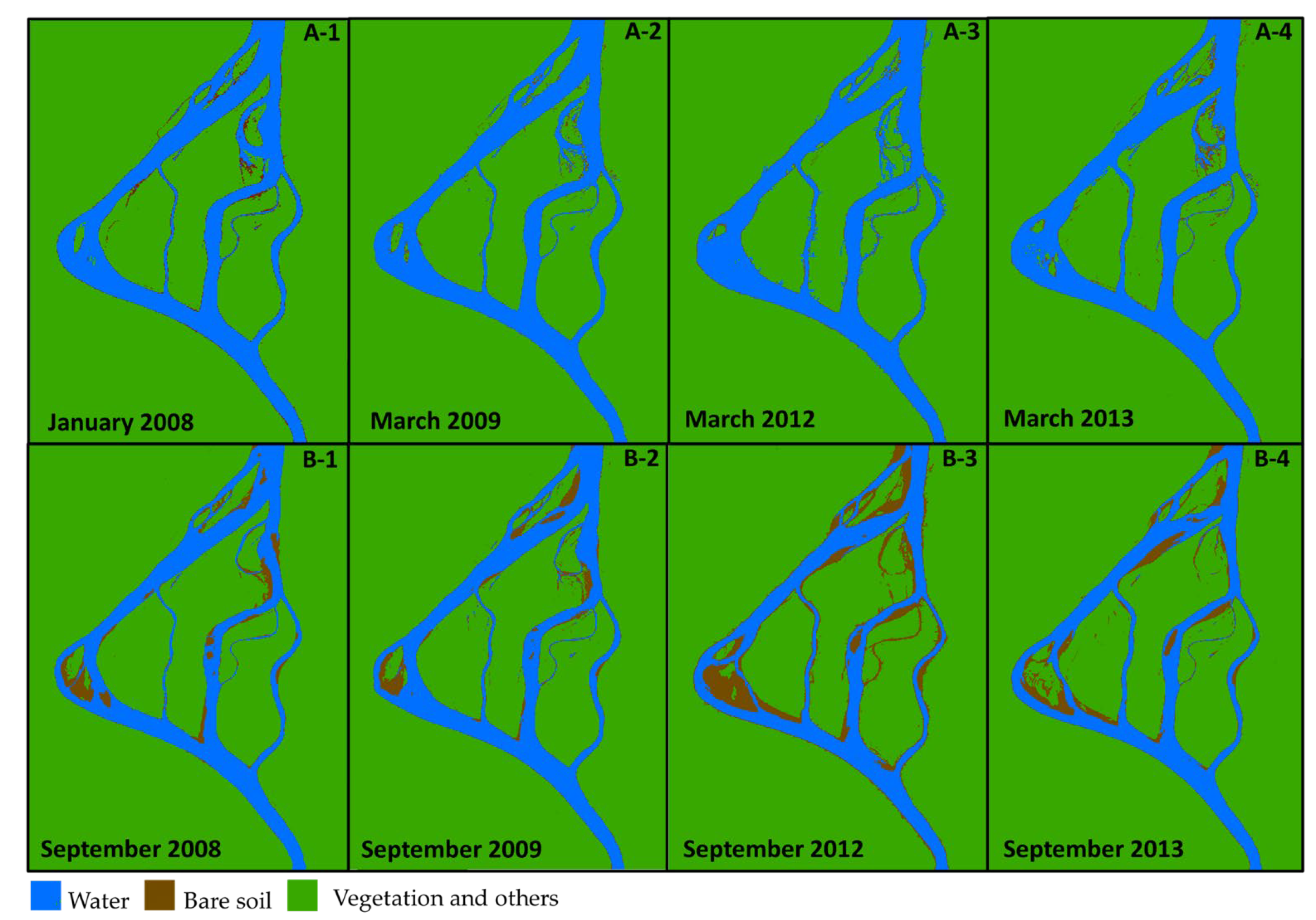
5.1. Seasonal Planform Change
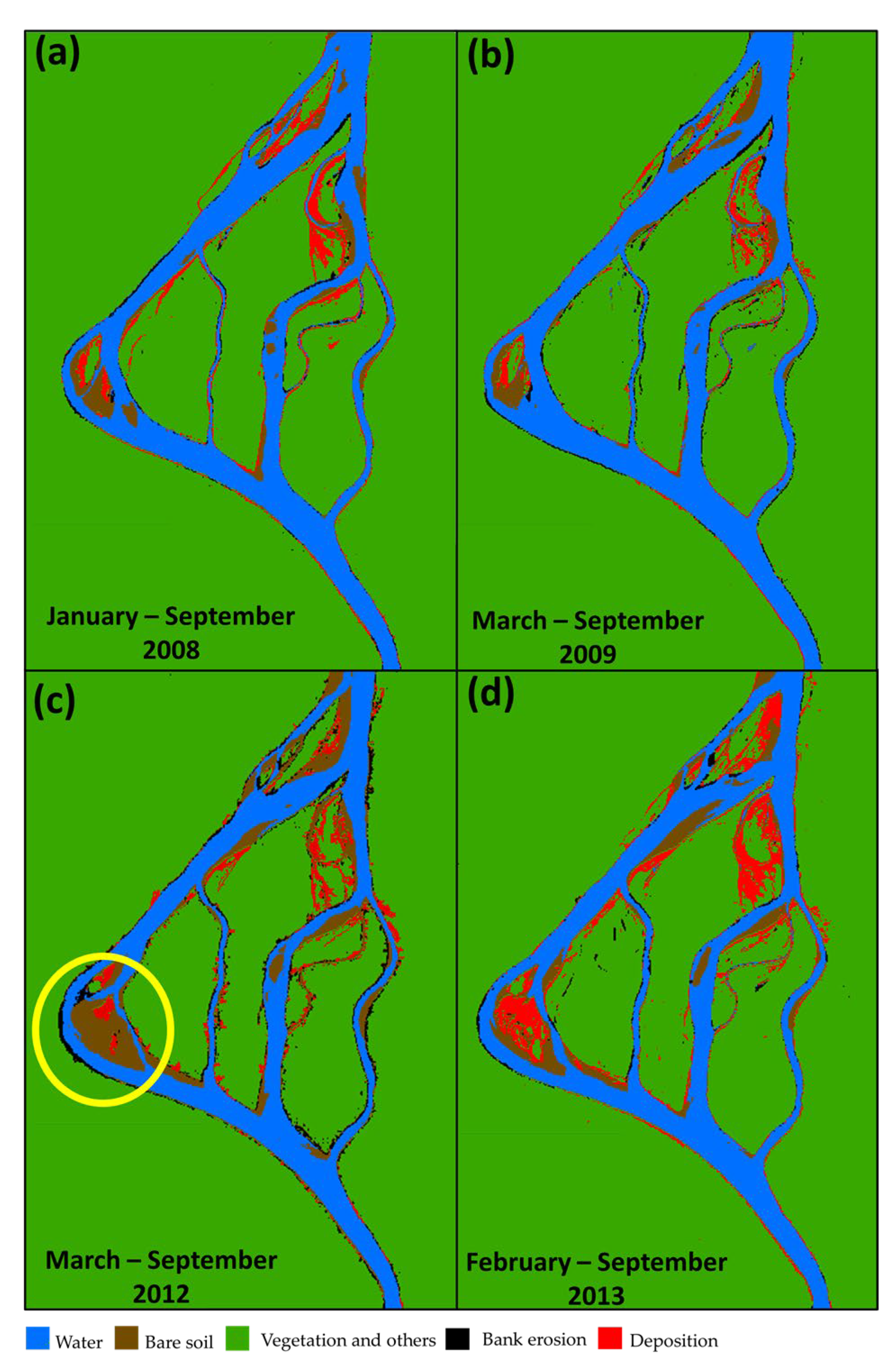
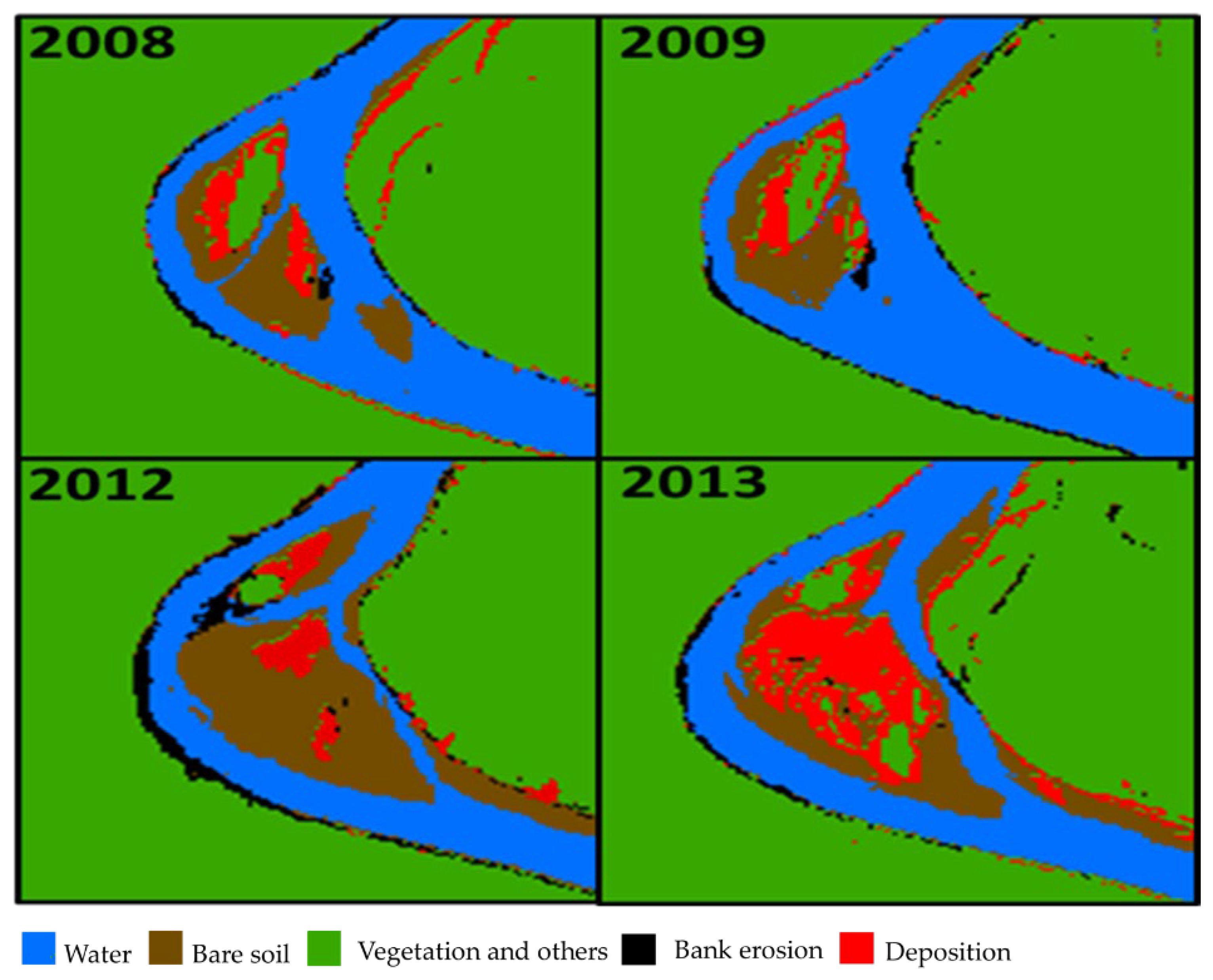
5.2. Influence of the 2012 Severe Flood
6. Conclusions
Author Contributions
Funding
Data Availability Statement
Acknowledgments
Conflicts of Interest
References
- Dunne, T.; Aalto, R.E. Large river floodplains. In Treatise on Geomorphology; Academic Press: Cambridge, MA, USA, 2013; Volume 9, pp. 645–678. [Google Scholar]
- Wohl, E. Hydrology and Discharge. In Large Rivers: Geomorphology and Management; Gupta, A., Ed.; John Wiley & Sons: Chichester, UK, 2007; pp. 29–41. [Google Scholar]
- Wynn, T.; Mostaghimi, S. The effects of vegetation and soil type on streambank erosion. Southwestern Virginia, USA. J. Am. Water Resour. Assoc. 2006, 42, 69–82. [Google Scholar] [CrossRef]
- Chatterjee, S.; Krishna, A.P. Geospatial assessment of soil erosion vulnerability at a watershed level in some sections of the Upper Subarnarekha river basin, Jharkhand, India. Environ. Earth Sci. 2014, 71, 357e374. [Google Scholar] [CrossRef]
- Daly, E.R.; Miller, R.B.; Fox, G.A. Modeling streambank erosion and failure along protected and unprotected composite streambanks. Adv. Water Resour. 2015, 81, 114–127. [Google Scholar] [CrossRef]
- Botero-Acosta, A.; Chua, M.L.; Guzman, J.A.; Starks, P.J.; Moriasi, D.N. Riparian erosion vulnerability model based on environmental features. J. Environ. Manag. 2017, 203, 592–602. [Google Scholar] [CrossRef] [PubMed]
- Sale, J.; Kalliola, R.; Hakkinen, I.; Makinen, Y.; Niemala, P.; Puhakka, M.; Coley, P.D. River dynamics and the diversity of Amazon lowland forest. Nature 1986, 322, 254–258. [Google Scholar] [CrossRef]
- Yang, X.; Damen, C.J.M.; Zuidam, A.R. Satellite remote sensing and GIS for the analysis of channel migration changes in the active Yellow River Delta, China. Int. J. Appl. Earth Obs. Geoinf. 1999, 1, 146–157. [Google Scholar] [CrossRef]
- Kummu, M.; Lu, X.X.; Rasphone, A.; Juha, S.; Jorma, K. Riverbank changes along the Mekong River: Remote sensing detection in the Vientiane—Nong Khai area. Quat. Int. 2008, 186, 100–112. [Google Scholar] [CrossRef] [Green Version]
- Hassan, M.S.; Mahmud-ul-islam, S. Quantification of River Bank Erosion and Bar Deposition in Chowhali Upazila, Sirajganj District of Bangladesh: A Remote Sensing Study. J. Geosci. Environ. Prot. 2016, 4, 50–57. [Google Scholar] [CrossRef] [Green Version]
- Jeong, Y.; Lee, K.J.; Chae, T.B.; Yu, J. Analysis of Tidal Channel Variations Using High Spatial Resolution Multispectral Satellite Image in Sihwa Reclaimed Land, South Korea. Korean J. Remote Sens. 2020, 36, 1605–1613. [Google Scholar]
- Kalliola, R.; Salo, J.; Puhakka, M.; Rajasilta, M.; Häme, T.; Neller, R.; Räsänen, M.; Danjoy, A.W. Upper Amazon channel migration. Implication for vegetation perturbance and succession using bitemporal Landsat MSS images. Naturwissenschaffen 1992, 79, 76–79. [Google Scholar]
- Rozo, M.G.; Nogueira, A.C.R.; Truckenbrodt, W. The anastomosing pattern and the extensively distributed scroll bars in the middle Amazon River. Earth Surf. Processes Landf. 2012, 37, 1471–1488. [Google Scholar] [CrossRef]
- Rozo, M.G.; Nogueira, A.C.R.; Castro, C.S. Remote sensing-based analysis of the planform changes in the Upper Amazon River over the period 1986–2006. J. S. Am. Earth Sci. 2014, 51, 28–44. [Google Scholar] [CrossRef]
- Frias, C.E.; Abad, J.D.; Mendoza, A.; Paredes, J.; Ortals, C.; Montoro, H. Planform evolution of two anabranching structures in the Upper Peruvian Amazon River. Water Resour. Res. 2015, 51, 2742–2759. [Google Scholar] [CrossRef]
- Mendoza, A.; Abad, J.D.; Frias, C.E.; Ortals, C.; Paredes, J.; Montoro, H.; Soto-Cortés, G. Planform dynamics of the Iquitos anabranching structure in the Peruvian Upper Amazon River. Earth Surf. Processes Landf. 2016, 41, 961–970. [Google Scholar] [CrossRef]
- Yen, C.L.; Lee, K.T. Bed topography and sediment sorting in channel bend with unsteady flow. J. Hydraul. Eng. ASCE 1995, 121, 591–599. [Google Scholar] [CrossRef]
- Lee, K.T.; Liu, Y.L.; Cheng, K.H. Experimental investigation of bed load transport processes under unsteady flow conditions. Hydrol. Process. 2004, 18, 2439–2454. [Google Scholar] [CrossRef]
- Puhakka, M.; Kalliola, R.; Rajasilta, M.; Salo, J. River Types, Site Evolution and Successional Vegetation Patterns in Peruvian Amazonia. J. Biogeogr. 1992, 19, 651. [Google Scholar] [CrossRef]
- Guan, M.; Wright, N.G.; Sleigh, P.A. Multiple effects of sediment transport and geomorphic processes within flood events: Modelling and understanding. Int. J. Sediment Res. 2015, 30, 371–381. [Google Scholar] [CrossRef]
- Karimaee Tabarestani, M.; Zarrati, A.R. Sediment transport during flood event: A review. Int. J. Environ. Sci. Technol. 2015, 12, 775–788. [Google Scholar] [CrossRef] [Green Version]
- Abad, J.D.; Frias, C.E.; Buscaglia, G.C.; Garcia, M.H. Modulation of the flow structure by progressive bedforms in the Kinoshita meandering channel. Earth Surf. Processes Landf. 2013, 38, 1612–1622. [Google Scholar] [CrossRef]
- Abad, J.D.; Paredes, J.; Montoro, H. Similarities and differences between a large meandering river and an ana-branching river: The Ucayali and Amazon River cases. In Proceedings of the 2010 Fall Meeting, AGU, San Francisco, CA, USA, 13–17 December 2010. EP24B-04. [Google Scholar]
- Abad, J.; Vizcarra, J.; Paredes, J.; Montoro, H. Morphodynamics of the upper Peruvian Amazonian rivers, implications into fluvial transportation. In Proceedings of the IDS 2013—First International Conference, Iquitos, Peru, 17–19 July 2013; pp. 1–10. [Google Scholar]
- Abad, J.D.; Garcia, M.H. Experiments in a high-amplitude Kinoshita meandering channel. 1: Implications of bend orientation on mean and turbulent flow structure. Water Resour. Res. 2009, 45, W02401. [Google Scholar] [CrossRef] [Green Version]
- Abad, J.D.; Garcia, M.H. Experiments in a high-amplitude Kinoshita meandering channel. 2: Implications of bend orientation on bed morphodynamics. Water Resour. Res. 2009, 45, W02402. [Google Scholar] [CrossRef]
- Mertes, L.A.; Dunne, T.; Martinelli, L.A. Channel-floodplain geomorphology along the Solimoes-Amazon River, Brazil. GSA Bull. 1996, 108, 1089–1107. [Google Scholar] [CrossRef]
- Arce-Nazario, J. Landscape Javier A. Images in Amazonian Narrative: The Role of Oral History in Environmental Research. Conserv. Soc. 2007, 5, 115–133. [Google Scholar]
- Armijos, E.; Crave, A.; Vauchel, P.; Fraizy, P.; Santini, W.; Moquet, J.-S.; Guyot, J.-L. Suspended sediment dynamics in the Amazon River of Peru. J. S. Am. Earth Sci. 2013, 44, 75–84. [Google Scholar] [CrossRef]
- Pinedo-Vasquez, M.; Barletti Pasqualle, J.; Del Castillo Torres, D.; Coffey, K. A tradition of change: The dynamic relationship between biodiversity and society in sector Muyuy, Peru. Environ. Sci. Policy 2002, 5, 43–53. [Google Scholar] [CrossRef]
- Rebata, L.A.; Gingras, M.K.; Räsänen, M.E.; Barberi, M. Tidal-channel deposits on a delta plain from the Upper Miocene Nauta Formation, Maranon Foreland Sub-basin, Peru. Sedimentology 2006, 53, 971–1013. [Google Scholar] [CrossRef]
- Räsänen, M.; Linna, A.; Irion, G.; Rebata, L.; Vargas, R.; Wesselingh, F.; Geología, Y. Geoformas de la zona de Iquitos. In Geoecología y Desarrollo Amazónico: Estudio Integrado en la Zona de Iquitos, Perú; Kalliola, R., Flores Paitán, S., Eds.; University of Turku: Turku, Finland, 1998; Volume 114, pp. 59–137. [Google Scholar]
- Siiro, P.; Räsänen, M.; Gingras, M.; Harris, C.; Irion, G.; Pemberton, S.G.; Ranzi, A. Application of laser diffraction grain-size analysis to reveal depositional processes in tidally-influenced systems. In Fluvial Sedimentology VII, IAS Special Publication; Blum, M., Marriott, S., Leclair, S., Eds.; Blackwell Publishing: Oxford, UK, 2005; Volume 35, pp. 159–180. [Google Scholar]
- Marengo, J.A.; Espinoza, J.C. Extreme seasonal droughts and floods in Amazonia: Causes, trends and impacts. Int. J. Climatol. 2015, 36, 1033–1050. [Google Scholar] [CrossRef]
- Zhang, R.; Tang, X.; You, S.; Duan, K.; Xiang, H.; Luo, H. A novel feature-level fusion framework using optical and SAR remote sensing images for land use/land cover (LULC) classification in cloudy mountainous area. Appl. Sci. 2020, 10, 2928. [Google Scholar] [CrossRef]
- Ling, J.; Zhang, H.; Lin, Y. Improving Urban Land Cover Classification in Cloud-Prone Areas with Polarimetric SAR Images. Remote Sens. 2021, 13, 4708. [Google Scholar] [CrossRef]
- Chavez, P.S., Jr. Image-based atmospheric corrections—Revisited and improved. Photogramm. Eng. Remote Sens. 1996, 62, 1025–1036. [Google Scholar]
- Milanović, M.M.; Micić, T.; Lukić, T.; Nenadović, S.S.; Basarin, B.; Filipović, D.J.; Tomić, M.; Samardžić, I.; Srdić, Z.; Nikolić, G.; et al. Application of Landsat-derived NDVI in monitoring and assessment of vegetation cover changes in Central Serbia. Carpathian J. Earth Environ. Sci. 2019, 14, 119–129. [Google Scholar] [CrossRef]
- Groeneveld, D.P.; Baugh, W.M. Correcting satellite data to detect vegetation signal for eco-hydrologic analyses. J. Hydrol. 2007, 344, 135–145. [Google Scholar] [CrossRef]
- Jensen, J.R. Introductory Digital Image Processing: A Remote Sensing Perspective, 3rd ed.; Prentice-Hall: Upper Saddle River, NJ, USA, 2005; pp. 505–512. [Google Scholar]
- Yüksel, A.; Akay, A.; Gundogan, R. Using ASTER Imagery in Land Use/cover Classification of Eastern Mediterranean Landscapes According to CORINE Land Cover Project. Sensors 2008, 8, 1237–1251. [Google Scholar] [CrossRef] [Green Version]
- Wu, Y.; Li, W.; Wang, Q.; Yan, S. Landslide susceptibility assessment using frequency ratio, statistical index and certainty factor models for the Gangu County, China. Arab. J. Geosci. 2016, 9, 84. [Google Scholar] [CrossRef]
- Gyssels, G.; Poesen, J.; Bochet, E.; Li, Y. Impact of plant roots on the resistance of soils to erosion by water: A review. Prog. Phys. Geogr. 2005, 29, 189–217. [Google Scholar] [CrossRef] [Green Version]
- De Baets, S.; Poesen, J.; Knapen, A.; Barberá, G.G.; Navarro, J.A. Root characteristics of representative Mediterranean plant species and their erosion-reducing potential during concentrated runoff. Plant Soil 2007, 294, 169–183. [Google Scholar] [CrossRef]
- Li, X.-L.; Marschner, H.; George, E. Acquisition of phosphorus and copper by VA-mycorrhizal hyphae and root to shoot transport in white clover. Plant Soil 1991, 136, 49–57. [Google Scholar] [CrossRef]
- Zhou, Z.C.; Shangguan, Z.P. Soil anti-scouribility enhanced by plant roots. J. Integr. Plant Biol. 2005, 47, 676–682. [Google Scholar] [CrossRef]
- De Baets, K.; Klug, C.; Korn, D. Anetoceratinae (Ammonoidea, Early Devonian) from the Eifel and Harz Mountains (Germany), with a revision of their genera. Neues Jahrb. Für Geol. Paläontologie Abh. 2009, 252, 361–376. [Google Scholar] [CrossRef]
- Vannoppen, W.; Vanmaercke, M.; DeBaets, S.; Poesen, J. A review of the mechanical effects of plant roots on concentrated flow erosion rates. Earth Sci. Rev. 2015, 150, 666–678. [Google Scholar] [CrossRef] [Green Version]
- Gross, D. Monitoring Agricultural Biomass Using NDVI Time Series; Food and Agriculture Organization of the United Nations (FAO): Rome, Italy, 2005. [Google Scholar]
- Montandon, L.; Small, E. The impact of soil reflectance on the quantification of the green vegetation fraction from NDVI. Remote Sens. Environ. 2008, 112, 1835–1845. [Google Scholar] [CrossRef]
- Ortega-Martin, P.; García-Montero, L.G.; Sibelet, N. Temporal Patterns in Illumination Conditions and Its Effect on Vegetation Indices Using Landsat on Google Earth Engine. Remote Sens. 2020, 12, 211. [Google Scholar] [CrossRef] [Green Version]
- Wang, Y.; Colby, J.D.; Mulcahy, K.A. An efficient method for mapping flood extent in a coastal flood plain using Landsat TM and DEM data. Int. J. Remote Sens. 2002, 23, 3681–3696. [Google Scholar] [CrossRef]
- Sanyal, J.; Lu, X.X. Application of Remote Sensing in Flood Management with Special Reference to Monsoon Asia: A Review. Nat. Hazards 2004, 33, 283–301. [Google Scholar] [CrossRef]
- Al-Doski, J.; Shattri, B.; Zulhaidi, M. NDVI Differencing and Post-classification to Detect Vegetation Changes in Halabja City, Iraq. IOSR J. Appl. Geol. Geophys. 2013, 1, 1–10. [Google Scholar] [CrossRef]
- Sharma, N.; Akhtar, M.P.; Zeleke, B. Satellite Data Based Impact Assessment of Basin Characteristics for Brahmaputra River System of India. In Proceedings of the World Environmental and Water Resources Congress, Palm Springs, CA, USA, 22–26 May 2011. [Google Scholar]
- Aalto, R.; Lauer, J.W.; Dietrich, W.E. Spatial and temporal dynamics of sediment accumulation and exchange along Strickland River floodplains (Papua New Guinea) over decadal-to-centennial timescales. J. Geophys. Res. 2008, 113, F01S04. [Google Scholar] [CrossRef] [Green Version]
- Fisher, G.B.; Bookhagen, B.; Amos, C.B. Channel planform geometry and slopes from freely available high-spatial resolution imagery and DEM fusion: Implications for channel width scalings, erosion proxies, and fluvial signatures in tectonically active landscapes. Geomorphology 2013, 194, 46–56. [Google Scholar] [CrossRef]
- Gurnell, A. Adjustments in river channel geometry associated with hydraulic discontinuities across the fluvial-tidal transition of a regulated river. Earth Surf. Process. Landform. 1997, 22, 967–985. [Google Scholar] [CrossRef]
- Gurnell, A.M. Channel change on the River Dee meanders, 1946–1992, from the analysis of air photographs. Regul. Rivers Res. Manag. 1997, 13, 13–26. [Google Scholar] [CrossRef]
- Lauer, J.W.; Parker, G. Net local removal of floodplain sediment by river meander migration. Geomorphology 2008, 96, 123–149. [Google Scholar] [CrossRef]
- Mount, N.; Louis, J. Estimation and propagation of error in measurements of river channel movement from aerial imagery. Earth Surf. Process. Landform. 2005, 30, 635–643. [Google Scholar] [CrossRef]
- Peixoto, J.M.A.; Nelson, B.W.; Wittmann, F. Spatial and temporal dynamics of river channel migration and vegetation in central Amazonian white-water floodplains by remote-sensing techniques. Remote Sens. Environ. 2009, 113, 2258–2266. [Google Scholar] [CrossRef]
- Richard, G.A.; Julien, P.Y.; Baird, D.C. Statistical analysis of lateral migration of the Rio Grande, New Mexico. Geomorphology 2005, 71, 139–155. [Google Scholar] [CrossRef] [Green Version]
- Winterbottom, S.J.; Gilvear, D.J. A GIS-based approach to mapping probabilities of river bank erosion: Regulated River Tummel, Scotland. Regul. Rivers Res. Manag. 2000, 16, 127–140. [Google Scholar] [CrossRef]
- Gurnell, A.M.; Downward, S.R.; Jones, R. Channel planform change on the River Dee meanders, 1876–1992. Regul. Rivers Res. Manag. 1994, 9, 187–204. [Google Scholar] [CrossRef]
- Brumby, S.P.; Theiler, J.; Perkins, S.J.; Harvey, N.J.; Szymanski, J.J.; Bloch, J.J.; Mitchell, M. Investigation of image feature extraction by a genetic algorithm. In Proceedings of the SPIE’s International Symposium on Optical Science, Engineering, and Instrumentation, Applications and Science of Neural Networks, Fuzzy Systems, and Evolutionary Computation II. International Society for Optics and Photonics, Denver, CO, USA, 18 July 1999; Volume 3812, pp. 24–31. [Google Scholar] [CrossRef] [Green Version]
- Dey, A.; Bhattacharya, R.K. Monitoring of river center line and width—A study on river Brahmaputra. J. Indian Soc. Remote Sens. 2014, 42, 475–482. [Google Scholar] [CrossRef]
- Dillabaugh, C.R.; Niemann, K.O.; Richardson, D.E. Semi-automated extraction of rivers from digital imagery. GeoInformatica 2002, 6, 263–284. [Google Scholar] [CrossRef]
- Hamilton, S.K.; Kellndorfer, J.; Lehner, B.; Tobler, M. Remote sensing of floodplain geomorphology as a surrogate for biodiversity in a tropical river system (Madre de Dios, Peru). Geomorphology 2007, 89, 23–38. [Google Scholar] [CrossRef]
- Marra, W.A.; Kleinhans, M.G.; Addink, E.A. Network concepts to describe channel importance and change in multichannel systems: Test results for the Jamuna River, Bangladesh. Earth Surf. Process. Landf. 2014, 39, 766–778. [Google Scholar] [CrossRef]
- McFeeters, S. The use of the Normalized DifferenceWater Index (NDWI) in the delineation of open water features. Int. J. Remote Sens. 1996, 17, 1425–1432. [Google Scholar] [CrossRef]
- Merwade, V.M. An automated GIS procedure for delineating river and lake boundaries. Trans. GIS 2007, 11, 213–231. [Google Scholar] [CrossRef]
- Quackenbush, L.J. A review of techniques for extracting linear features from imagery. Photogramm. Eng. Remote Sens. 2004, 70, 1383–1392. [Google Scholar] [CrossRef] [Green Version]
- Smith, L.C.; Pavelsky, T.M. Estimation of river discharge, propagation speed, and hydraulic geometry from space: Lena River, Siberia. Water Resour. Res. 2008, 44, W03427. [Google Scholar] [CrossRef]
- Xu, H. Modification of normalized difference water index (NDWI) to enhance open water features in remotely sensed imagery. Int. J. Remote Sens. 2006, 27, 3025–3033. [Google Scholar] [CrossRef]
- Zolezzi, G.; Luchi, R.; Tubino, M. Modeling morphodynamic processes in meandering rivers with spatial width variations. Rev. Geophys. 2012, 50, RG4005. [Google Scholar] [CrossRef] [Green Version]
- Rowland, J.C.; Shelef, E.; Pope, P.A.; Muss, J.; Gangodagamage, C.; Brumby, S.P.; Wilson, C.J. A morphology independent methodology for quantifying planview river change and characteristics from remotely sensed imagery. Remote Sens. Environ. 2016, 184, 212–228. [Google Scholar] [CrossRef] [Green Version]
- Downward, S.; Gurnell, A.; Brookes, A. A methodology for quantifying river channel planform change using GIS. IAHS Publications—Series of Proceedings and Reports; International Association of Hydrological Sciences: Wallingford, Oxfordshire, UK, 1994; Volume 224, pp. 449–456. [Google Scholar]

| Mission | Sensor | Date | Bands | Season | Annual Maximum Water Level (Meters above Sea Level; m.a.s.l) |
|---|---|---|---|---|---|
| L-7 L-5 | ETM+ TM+ | 11 January 2008 15 September 2008 | B3,B4 B3,B4 | Wet Dry | 116.80 |
| L-5 L-5 | TM+ TM+ | 26 March 2009 2 September 2009 | B3,B4 B3,B4 | Wet Dry | 117.73 |
| L-7 L-7 | ETM+ ETM+ | 26 March 2012 18 September2012 | B3,B4 B3,B4 | Wet Dry | 118.97 |
| L-7 L-7 | ETM+ ETM+ | 25 February2013 21 September2013 | B3,B4 B3,B4 | Wet Dry | 117.99 |
| N° | Station | UTM Coordinates | Geographical Coordinates | Geoidal Elevation | Signal |
|---|---|---|---|---|---|
| 1 | Tamshiyacu | 9557248.285 N 704161.971 E | 4°00′12.8816″ S 73°09′39.9759″ W | 98.914 | Geographical landmark |
| 2 | Iquitos | 9586988.403 N 695426.947 E | 3°44′05.3642″ S 73°14′25.1186″ W | 90.063 | Geographical landmark |
| Year | Areas in the Wet/Dry Seasons | ||
|---|---|---|---|
| Water (km2) | Bare Soil (km2) | Vegetation and Others (km2) | |
| 2008 | 83.32/69.54 | 6.20/12.07 | 462.54/470.46 |
| 2009 | 84.52/73.42 | 4.67/12.31 | 462.87/466.33 |
| 2012 | 89.81/62.11 | 5.65/31.00 | 456.60/458.96 |
| 2013 | 87.72/64.37 | 7.98/18.04 | 456.36/469.65 |
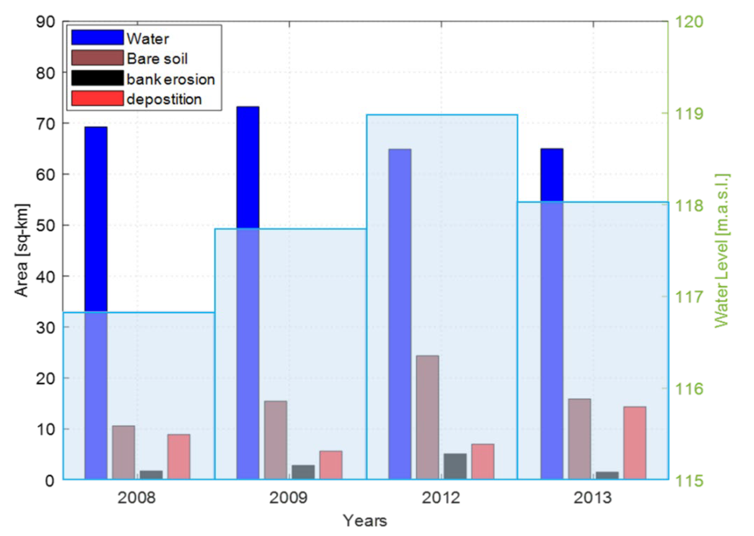
| Bank Erosion (km2) | Deposition (km2) | Annual Maximum Water Level (m.a.s.l) | |
|---|---|---|---|
| 2008 | 1.76 | 8.92 | 116.80 |
| 2009 | 2.85 | 5.64 | 117.73 |
| 2012 | 5.11 | 7.03 | 118.97 |
| 2013 | 1.54 | 14.36 | 117.99 |
Publisher’s Note: MDPI stays neutral with regard to jurisdictional claims in published maps and institutional affiliations. |
© 2022 by the authors. Licensee MDPI, Basel, Switzerland. This article is an open access article distributed under the terms and conditions of the Creative Commons Attribution (CC BY) license (https://creativecommons.org/licenses/by/4.0/).
Share and Cite
Garcia Angulo, K.; Lee, K.T. Detecting the Planform Changes Due to the Seasonal Flow Fluctuation and 2012 Severe Flood in the Amazon River near Iquitos City, Peru Based on Remote Sensing Image Analysis. Water 2022, 14, 509. https://doi.org/10.3390/w14030509
Garcia Angulo K, Lee KT. Detecting the Planform Changes Due to the Seasonal Flow Fluctuation and 2012 Severe Flood in the Amazon River near Iquitos City, Peru Based on Remote Sensing Image Analysis. Water. 2022; 14(3):509. https://doi.org/10.3390/w14030509
Chicago/Turabian StyleGarcia Angulo, Karen, and Kwan Tun Lee. 2022. "Detecting the Planform Changes Due to the Seasonal Flow Fluctuation and 2012 Severe Flood in the Amazon River near Iquitos City, Peru Based on Remote Sensing Image Analysis" Water 14, no. 3: 509. https://doi.org/10.3390/w14030509
APA StyleGarcia Angulo, K., & Lee, K. T. (2022). Detecting the Planform Changes Due to the Seasonal Flow Fluctuation and 2012 Severe Flood in the Amazon River near Iquitos City, Peru Based on Remote Sensing Image Analysis. Water, 14(3), 509. https://doi.org/10.3390/w14030509