Article

Baseflow Separation Using the Digital Filter Method: Review and Sensitivity Analysis

1
Disaster Prevention Research Institute, Pukyong National University, Busan 48513, Korea
2
Department of Civil Engineering, Pukyong National University, Busan 48513, Korea
3
Department of Civil Engineering, Kyungsung University, Busan 48434, Korea
*
Author to whom correspondence should be addressed.
Water 2022, 14(3), 485; https://doi.org/10.3390/w14030485
Submission received: 27 December 2021 / Revised: 30 January 2022 / Accepted: 3 February 2022 / Published: 7 February 2022
(This article belongs to the Special Issue Advances in Hydroinformatics for Water Data Management and Analysis)

Abstract

:
The baseflow separation method based on a digital filter is a simple method for separating the baseflow from streamflow. Appropriate estimation of filter parameters is required to use the digital filter method for analysis. We carried out sensitivity analysis on four digital filter methods: Lyne–Hollick (LH), Chapman, Chapman and Maxwell (CM), and exponentially weighted moving average (EWMA). Furthermore, appropriate filter parameters were suggested for each method in this study. By applying them to 25 stage stations in the Nakdong River in the Republic of Korea, the four methods were evaluated. The results of the evaluation showed that the Chapman and CM methods had problems separating the baseflow during the dry seasons. The EWMA and LH methods were able to achieve reliable baseflow separation of the outcomes by selecting appropriate the filter parameters. Thus, the EWMA and LH methods can be used easily and reasonably among the digital filter methods that have one filter parameter.

1. Introduction

Baseflow is the portion of streamflow that contains delayed subsurface flow, and it is generally maintained by groundwater discharge [1]. Baseflow accounts for most of the streamflow during the dry season, which has a crucial impact on the water quality and aquatic ecosystems [2]. In other words, it is no exaggeration to say that the core of stream management during the dry season is baseflow management. It is not easy to measure baseflow directly because it is the flow rate from groundwater [3]. Therefore, there is a necessity for a baseflow separation method that can accurately separate the direct runoff and the baseflow from the measured streamflow data [4].
Baseflow can be obtained using mass-balance methods with tracers [5,6,7,8,9]. These methods usually require monitoring tracer concentrations (ions, isotopes, conductivity, etc.) in surface runoff, stream water, and groundwater, and tracers in different basins can perfectly reflect the hydrogeological conditions [10]. However, these methods are very laborious and expensive, especially for long-term field measurements [9,11].
Numerous non-tracer-based methods have been developed to estimate baseflow from streamflow without field measurements, such as graphical analysis methods, numerical simulation methods, and digital filter methods [11,12]. Digital filter methods especially separate surface runoff (i.e., high-frequency signals) and baseflow (i.e., low-frequency signals) from the daily streamflow records, according to a digital filter [12]. In other words, the digital filter methods estimate baseflow by signal analysis with the assumption that baseflow is the low-frequency part of streamflow [11].
Since Lyne and Hollick [13] first suggested the use of a digital filter (Lyne–Hollick method) to separate baseflow, the method has been used by Nathan and McMahon [14], Arnold and Allen [15], and Arnold et al. [16], for example [17]. In addition, many researchers have developed various types of techniques based on the method. Representative digital filter-based baseflow separation methods are as follows: the Chapman method proposed by Chapman [18], the Chapman and Maxwell (CM) method proposed by Chapman and Maxwell [19], the Eckhardt method proposed by Eckhardt [17], and the exponentially weighted moving average (EWMA) method developed by Tularam and Ilahee [20].
The digital filter methods have no physical meaning in baseflow separation [21] and the methods include one or more filter parameters. The result of baseflow separation is susceptible to the parameter’s variation [22]. To accurately separate the baseflow from streamflow with the digital filter methods, appropriate filter parameters must be estimated by trial and error, which act as a difficulty or limitation on their use. However, in most of the past studies on the baseflow separation with digital filter methods, the filter parameters, which are difficult to estimate objectively, were arbitrarily determined or estimated through simple calibration [9,11,23,24]. Although some studies partially include the contents of filter parameter determination [12,17,20,22], there has been no research that comprehensively analyzes the sensitivity according to filter parameters for various methods.
The objective of this paper is to review the applicability of baseflow separation methods based on a digital filter and to suggest an appropriate range of filter parameters based on sensitivity analysis. The research methods used are the Lyne–Hollick (LH), Chapman, CM, and EWMA methods. The four baseflow separation methods that have a single parameter can be easier to use than the others. The four methods were analyzed for sensitivity by computing baseflow index (BFI) according to filter parameters and characteristics of rivers (streams). The sensitivity analysis adopted in this study is the condition number (CN), which measures how much the output value can change for a small change in the input data. The digital filter methods were evaluated for applicability and appropriateness for baseflow separation by applying them to 25 stage stations where the flow rate was measured continuously for eight years or more.

2. Method

2.1. Baseflow Separation Methods Based on a Single Filter Parameter

2.1.1. Applied Methods

There are digital filter baseflow separation methods in various forms: LH, Chapman, Eckhardt, CM, EWMA, etc. These methods need one or more parameters to separate the baseflow from the streamflow time series. The results of a baseflow separation from the measured streamflow differ depending on the method and filter parameters. This study suggests the results of a sensitivity analysis and a review of the baseflow separation methods that are relatively easy to analyze and have a single filter parameter. The study methods are LH, Chapman, CM, and EWMA. Table 1 summarizes the baseflow separation by the digital filter method applied in this study. Lyne and Hollick [13] suggested the LH method, which is based on signature processing and separates the streamflow into direct runoff and baseflow. The Chapman method was improved from the LH method [18]. The CM method assumes the baseflow at time t to be the weighted average of the surface runoff at time t and the baseflow at time t−1 [25]. The EWMA method, which is a simple exponential smoothing model, can be practically easier to apply when compared to the others described [20].

2.1.2. Filter Parameters

The baseflow separated by digital filter methods depends on the filter parameter. Therefore, it is essential to estimate filter parameters to use digital filter-based baseflow separation methods.
The following is a summary of the filter parameters for each the four methods described. Chapman [18] criticized the LH method for providing theoretically incorrect results [11,23], and proposed the Chapman method based on the LH method. In addition, Chapman [18] suggested that a single value of 0.925 for the filter parameter α gave satisfactory baseflow separation for drainage area in the range from 4.2 to 210 km2. The equation of the CM method includes the recession constant value as a filter parameter β (Table 1). The recession constant value can be calculated by recession analysis [23]. Eckhardt [23] suggested a recession constant value 0.960 or 0.961 that afforded a basis for results of the recession analysis at 65 rivers. Tularam and Ilahee [20] suggested the EWMA method and the range of filter parameters. Tularam and Ilahee [20] used filter parameters in the range from 0.003 to 0.015.
Even though the filter parameters have been presented in past studies, these studies included filter parameters that can differ according to the river regime and characteristics of a watershed [11,13,14,18,20,26]. Furthermore, others that have studied LH, Chapman, and CM methods used filter parameters in a range from 0.9 to 0.99. We selected a range of parameters based on past studies for review and sensitivity analysis. The filter parameters of the LH, Chapman, and CM methods range from 0.9 to 0.99, and those of EWMA range from 0.003 to 0.015 (Table 2).

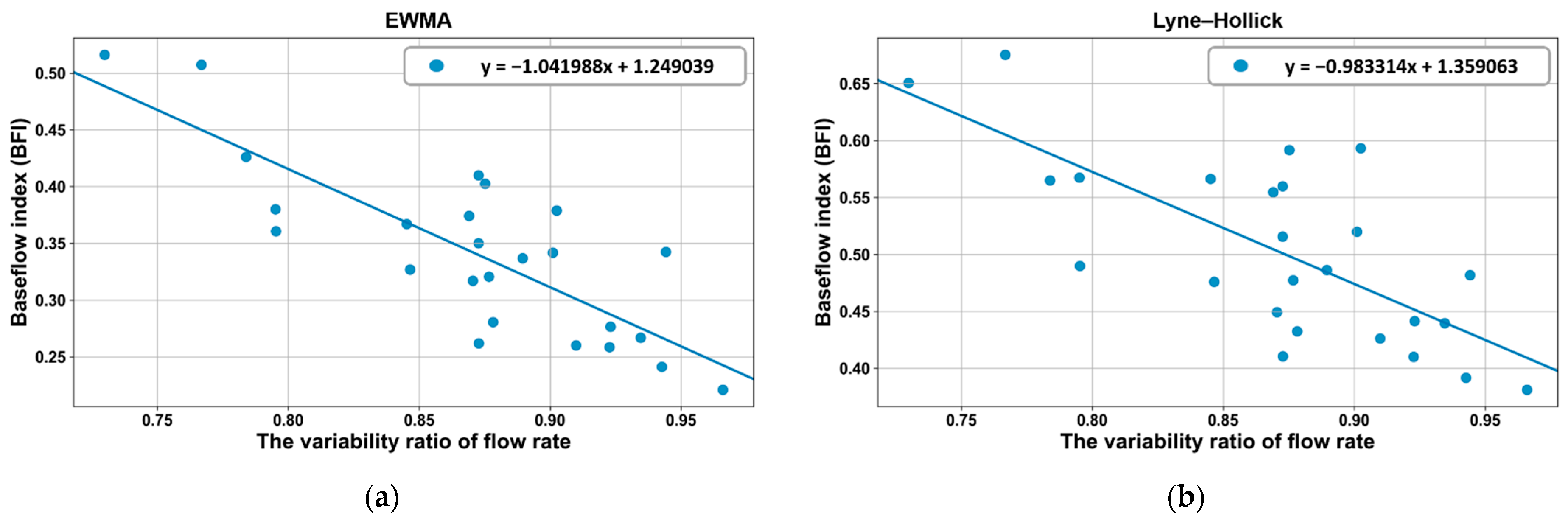
2.2. Sensitivity Analysis Method Considering Baseflow Index

2.2.1. Baseflow Index

Indicators are needed to analyze the variability in baseflow separation according to the change in filter parameters. The baseflow index (BFI) is one of the indicators for analyzing the results of baseflow separation. BFI is the ratio of the calculated baseflow volume to the measured streamflow volume over a specified period (Equation (1)). The equation of BFI is as follows:
B F I = Total   baseflow Total   streamflow

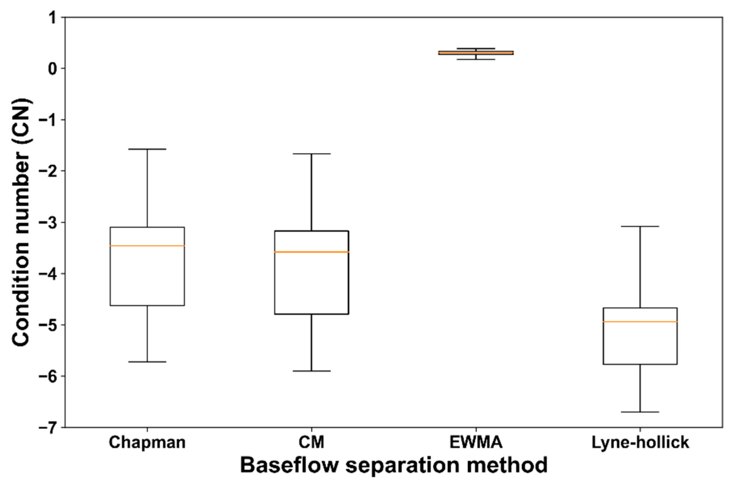
2.2.2. Condition Number

This study performed a sensitivity analysis to review variability in BFI according to the filter parameters. We performed this using the condition number (CNk) suggested by Chapra and Cannale [27] for sensitivity analysis. The equations of the condition number are as follows:
Δ c c = CN k Δ k k
CN k = k c c k
where CNk is the condition number for the parameter k, k is the inputted parameter, and c is the function of k. Equation (2) indicates that the condition number provides a transfer function to propagate the relative error of the parameter into the relative error of the result. The condition number is used to measure how sensitive a function of k is to changes in the parameter k. The absolute value of the condition number denotes the sensitivity of the function of k to the variability in parameter k. A positive or negative condition number means the function of k varies with either direct or inverse correlation to the variability of parameter k, respectively. In this study, the function of k is the BFI calculated from a baseflow separation method, and parameter k is a filter parameter.
On the other hand, sensitivity analysis using the condition number requires a value of the reference filter parameter. Therefore, in this study, five values were selected in the range of filter parameters (Table 3), and the intermediate value was adopted as the default value.

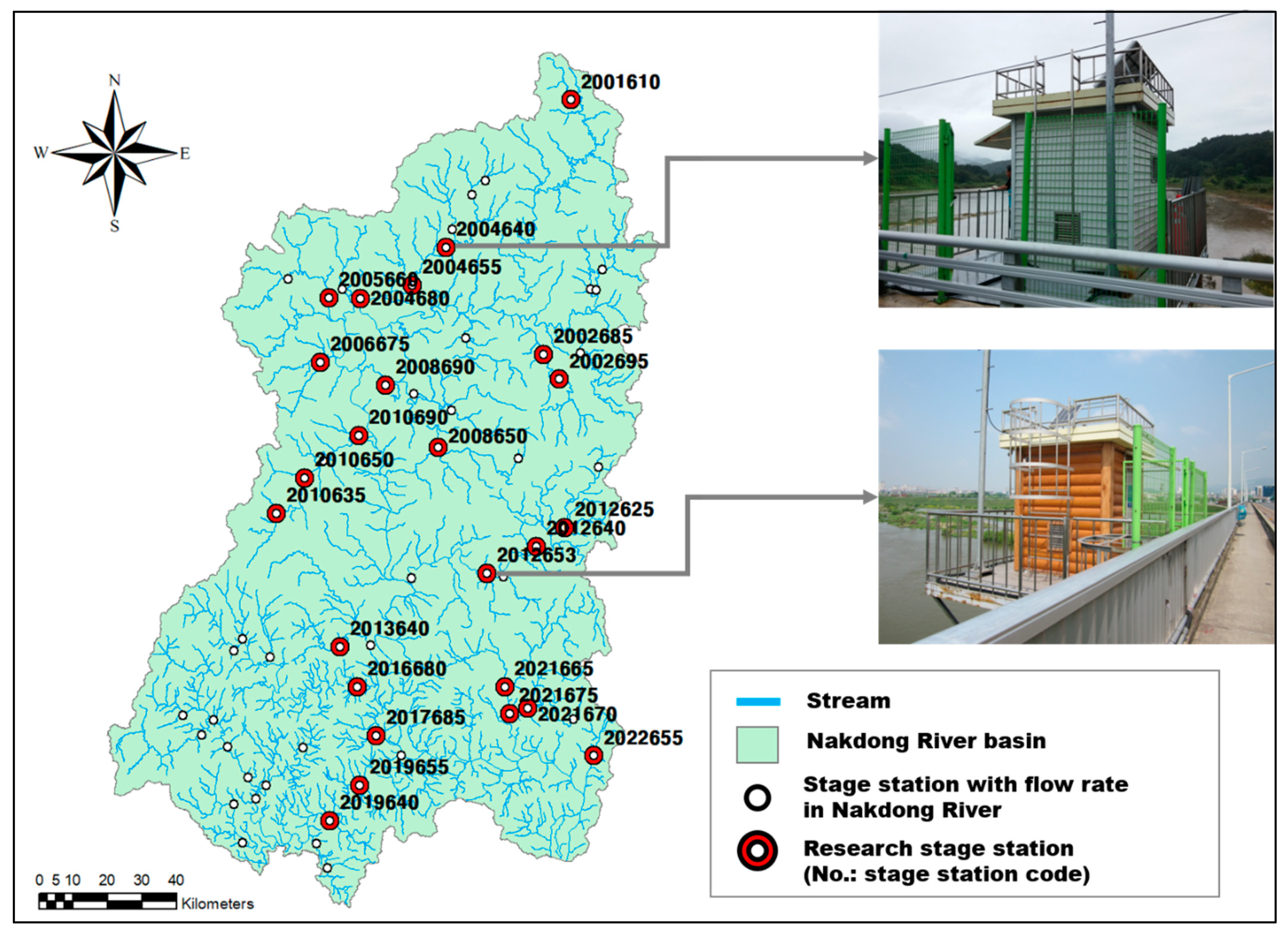
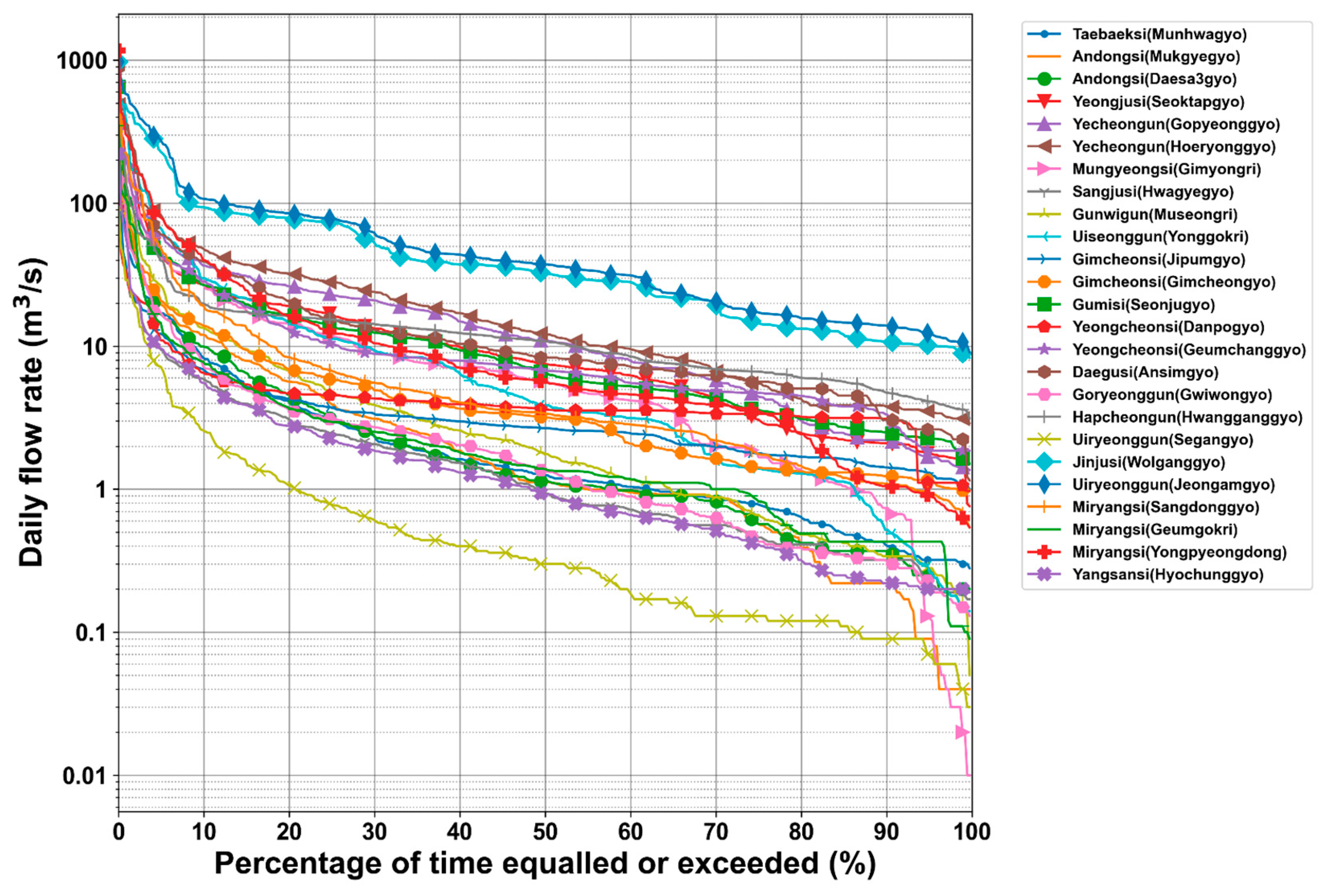
2.3. Target Station and Historical Streamflow Record

Sensitivity analysis and determining the appropriate range of filter parameters for baseflow separation methods require a long-term continuous streamflow record in a river. The four baseflow separation methods were applied to stage stations of Nakdong River in the Republic of Korea. There are 60 stage stations in Nakdong River, and we selected 25 of them to analyze the baseflow separation methods. The criterion for selecting the research stage stations was no missing values for more than 8 years among the last 20 years of the historical data.
Figure 1 shows the 60 stations (white circle) that include the studied stage stations (red donut) in the Nakdong River basin. As shown in Table 4, the studied stage stations have long-term daily measured streamflow data and the characteristics of a river regime. The coefficient of the river regime indicates the ratio between the maximum and minimum of a river. The coefficient of variation is the ratio of the standard deviation to the mean. The coefficients of the river regimes of the 25 study stations have various runoff characteristics that range from 88 to 1792, as shown in Table 4. These various values were caused by geomorphic and climatic characteristics of watershed.

3. Results

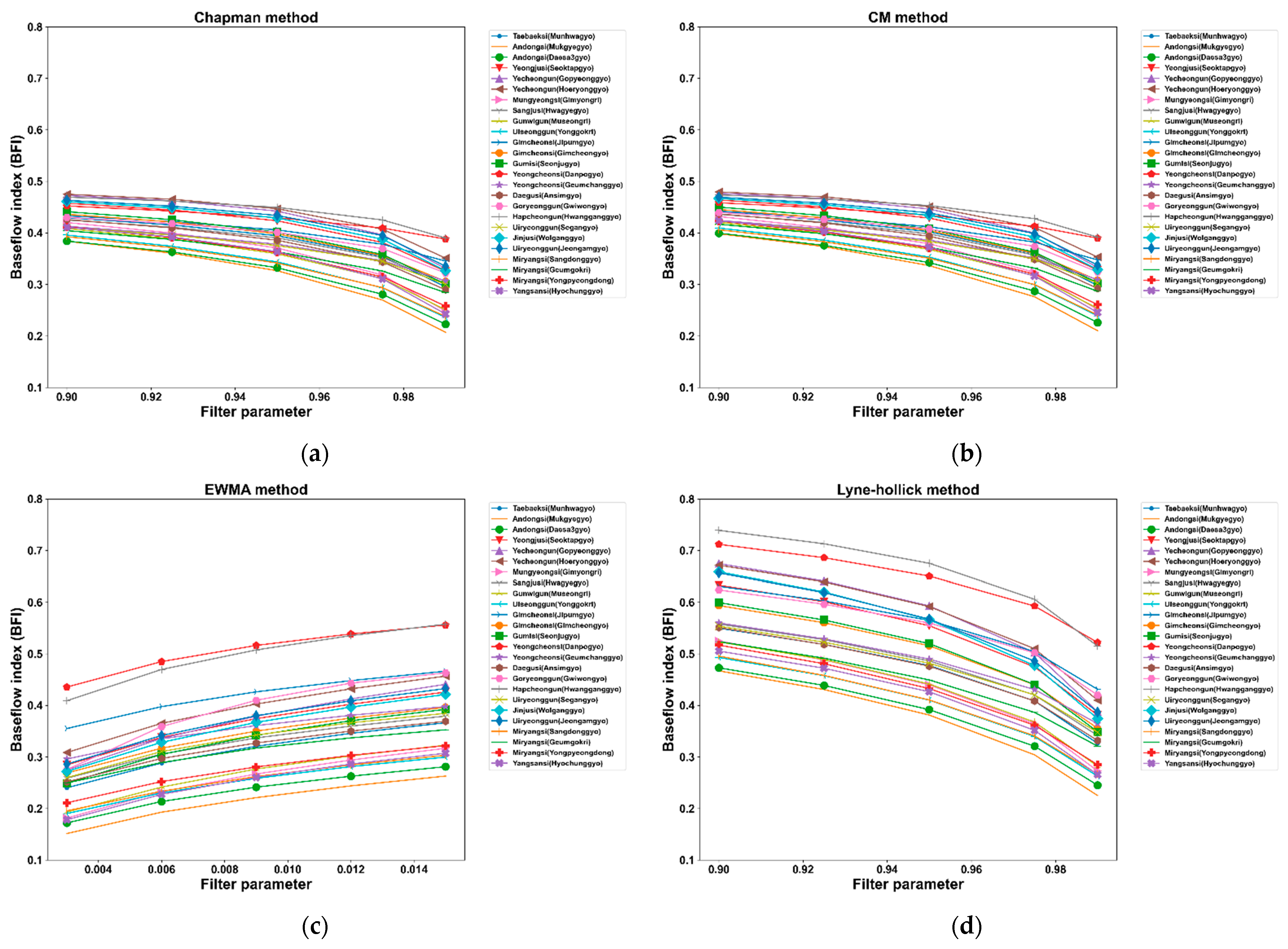
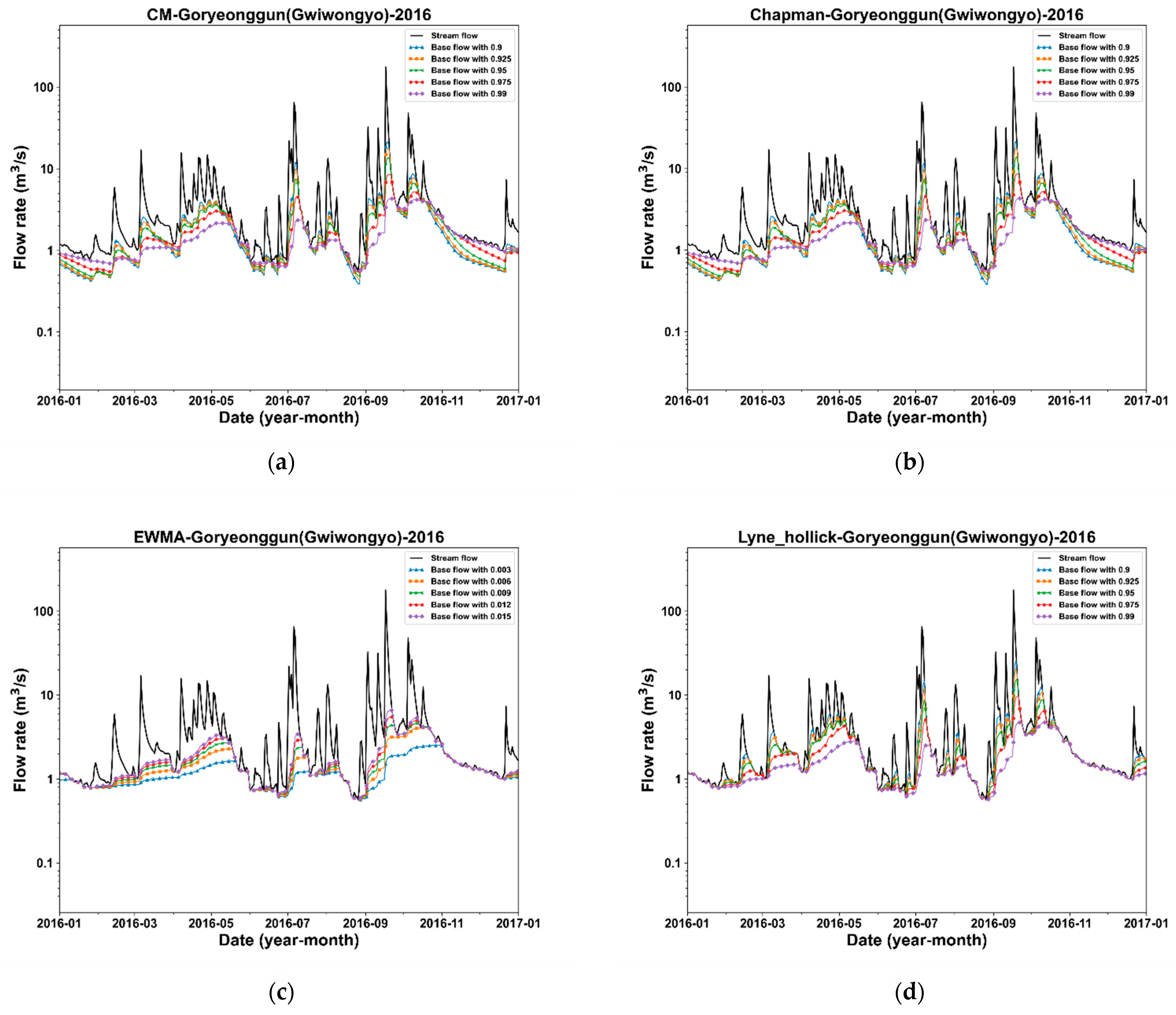
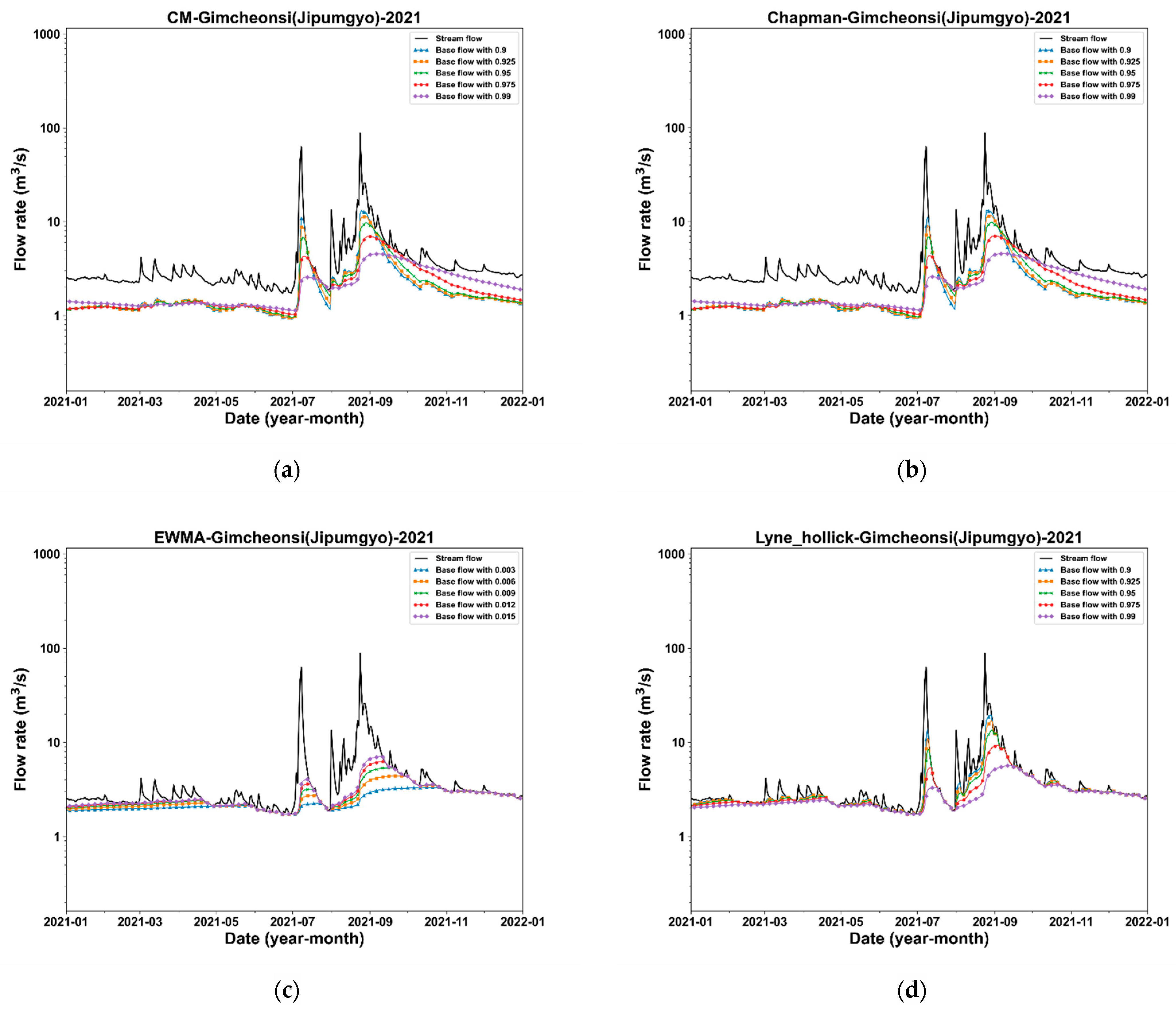
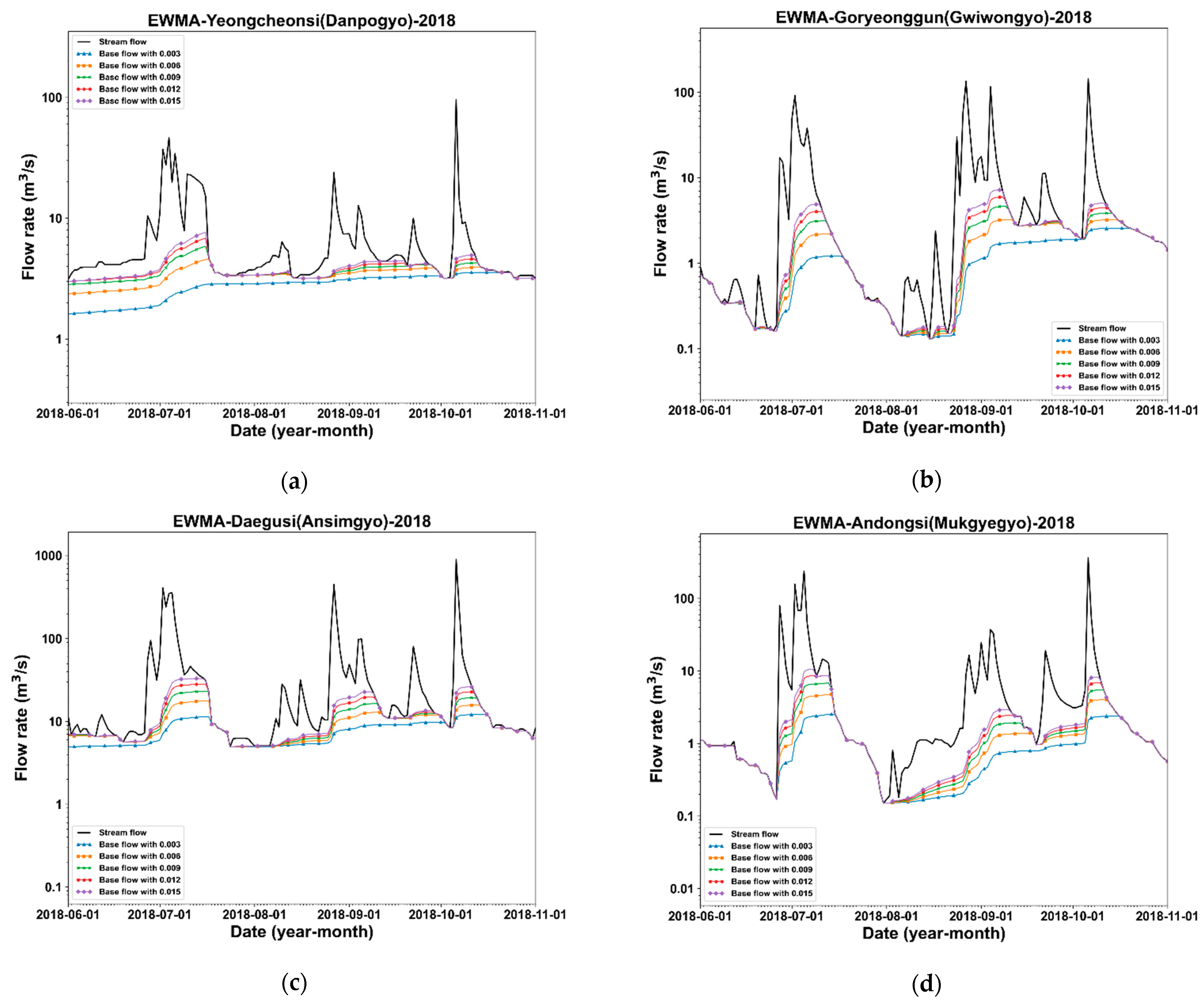
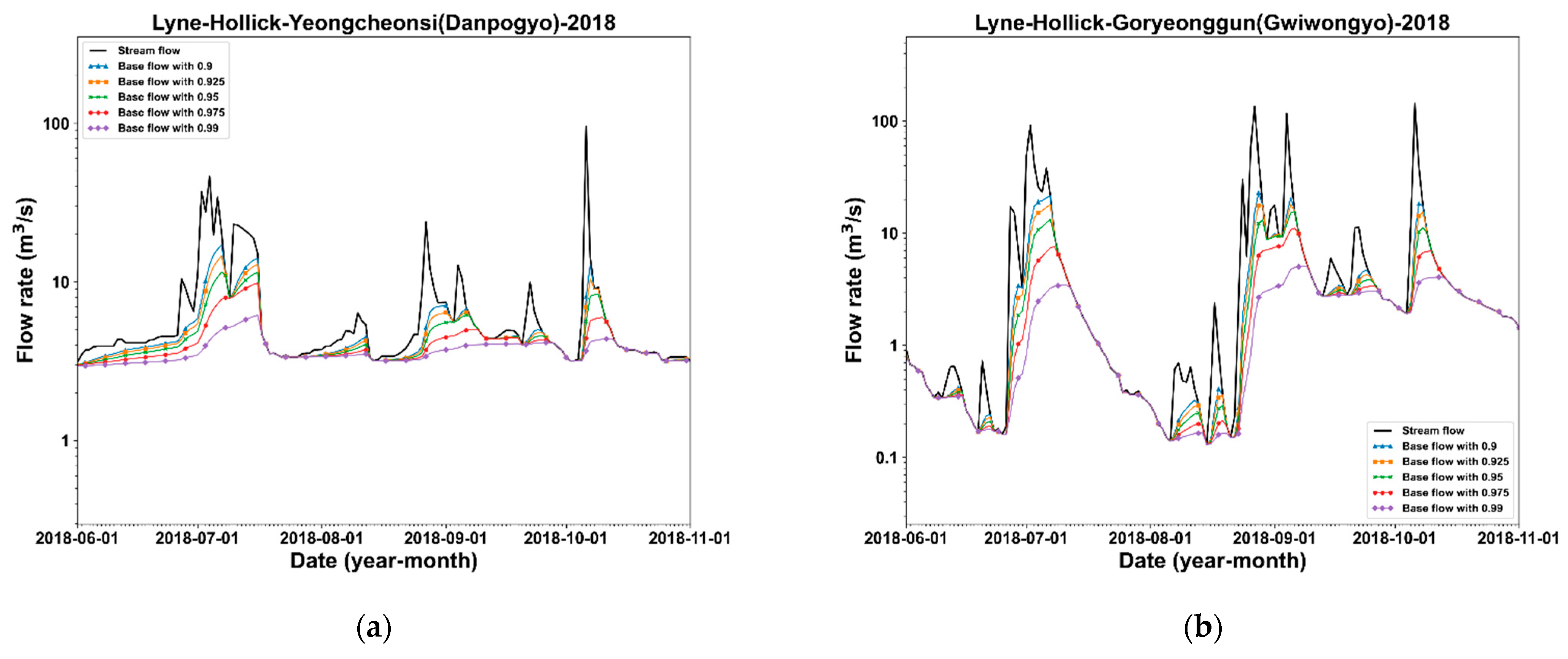
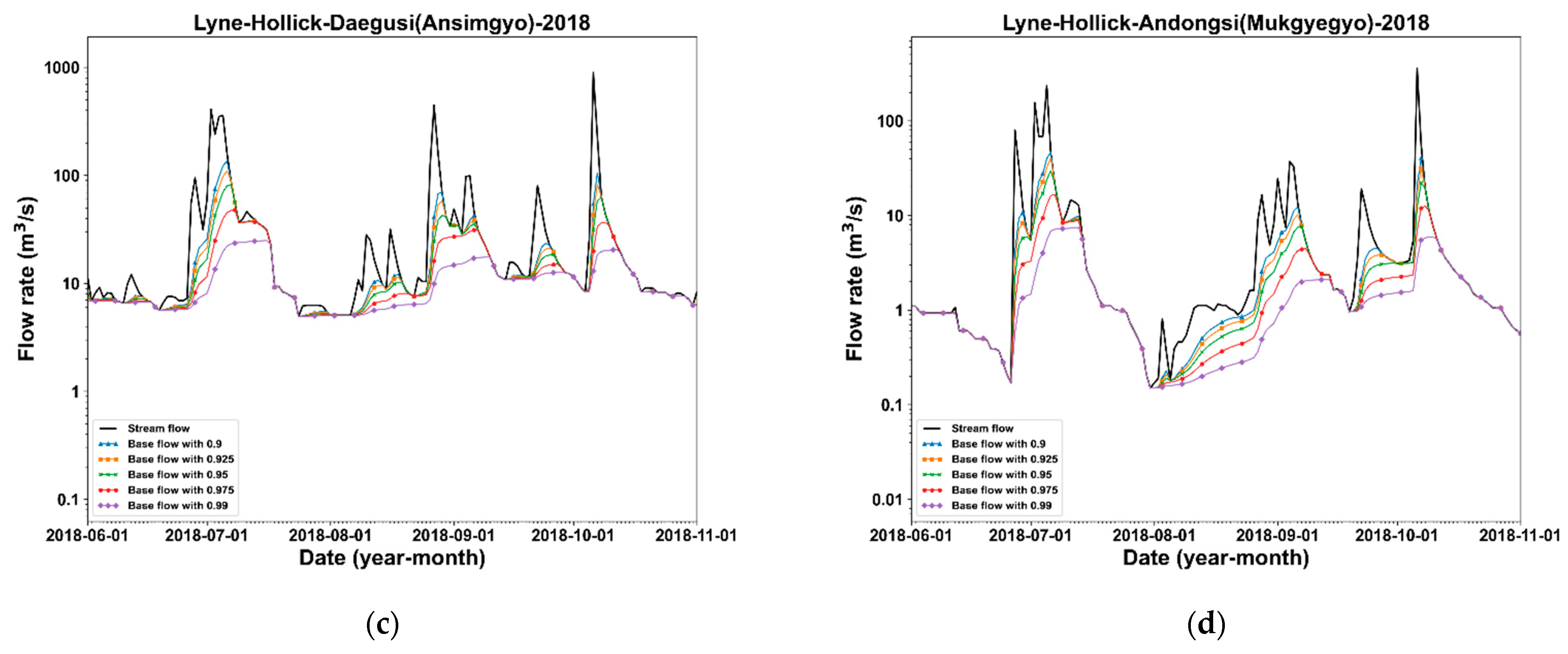
3.1. The Results of the Baseflow Separation by Filter Parameters

The authors compared the four baseflow separation methods based on their outcomes by filter parameter and the studied stage station shift. The applied filter parameter values of the Chapman, CM, and LH methods were 0.9, 0.925, 0.95, 0.975, and 0.99, and those for the EWMA method were 0.003, 0.006, 0.009, 0.012, and 0.015. Figure 2 and Figure 3 show the baseflow separation results of the methods. The baseflow separation outcomes by filter parameters of the Chapman and CM methods are similar. The Chapman, CM, and LH methods present smoother baseflow curves and smaller baseflow peaks as the filter parameter approaches 1. When the filter parameter approaches 0.9, they yield dynamic baseflow curves. It is especially notable that the baseflow separation outcomes of the Chapman and CM methods do not coincide with the recession curve during the dry season. This phenomenon occurs more clearly as the flow rate increases during the dry season. The baseflow separation outcomes of the EWMA and LH methods generally coincide with the recession curve.

3.2. Sensitivity Analysis Results

We analyzed the variance in the BFI according to the filter parameters. Figure 4 shows the BFI of the study stations calculated from the four methods with the filter parameters. As shown in Figure 4, the BFI of the Chapman, CM, and LH methods tend to decrease as the filter parameter increases. Conversely, the BFI of the EWMA method tends to increase as the filter parameter increases. The Chapman and CM methods show less variability in the BFI than the others in Figure 4. However, the watersheds of the study stations have various river regimes, which may be the basis for determining that the Chapman and CM methods do not consider the watershed characteristics. As shown in Figure 4c,d, the variance curves of the study stations from the EWMA and LH methods are relatively widely distributed. This phenomenon relates to several river characteristics of the stage stations. Figure 5 shows the flow duration curve of the study station in 2018. It can be seen that several flow duration curves have a high variability, e.g., Andongsi (Mukgyegyo, ‘orange line’) and Andongsi (Daesa3gyo, ‘green circle line’). We analyzed the relationship between BFI and the river characteristics of the study stations. The coefficient of the river regime and coefficient of the flow fluctuation are representative indicators of the river characteristics. However, the coefficient of the river regime has uncertain measurements for extreme flow rates (Qmin, Qmax). For this reason, we used the dimensionless variation as one of the watershed characteristics. The equation of dimensionless variation between QDi and QDj is as follows:
Q D i , D j = Q D i Q D j Q D i
where Di or Dj mean i-th or j-th deciles, QDi and QDj is the daily flow rate that equals or exceeds the i-th or j-th deciles of the time, and QDi,Dj is the dimensionless variation between QDi and QDj. The correlation coefficients between the BFI form the four methods and four cases of river characteristics of the study stations. The four cases of river characteristics are as follows: case (1) the dimensionless variation between QD1 and QD9; case (2) the dimensionless variation between QD2 and QD9; case (3) coefficient of river regime; case (4) coefficient of flow fluctuation. Table 5 shows the relationships between the BFI of the four methods from the study stations and the river characteristics of the study stations. The coefficient of the river regime is highly related to the four methods. The dimensionless variation (case 1) is highly related to the Chapman, CM, and LH methods and very highly related to the EWMA method (Figure 6). These results imply that the BFI of the four methods is likely to be negatively correlated with variability of the flow rate. As can be seen in Figure 4, the BFI of the EWMA and LH methods varies significantly for each stage station.
The condition number is used to measure how sensitive the BFI is to changes in the filter parameter. The larger the absolute value of a condition number, the more sensitive the BFI calculated from a baseflow separation method is to the parameter. Additionally, a negative condition number means that the BFI decreases as the parameter increases.
Table 6 shows condition numbers of the BFI for the study stations calculated from the baseflow separation methods. The LH method is the most sensitive to changes in the filter parameter among the four methods. The EWMA method is the most insensitive method. Figure 7 is a box–whisker plot of Table 6. It can be seen that the EWMA method has the smallest deviation in the condition numbers according to the station. Based on this result, it may be decided that the EWMA method is a convenient method to use among the baseflow separation methods.
As shown in Table 6, it can be seen that the sensitiveness of the BFI calculated by the baseflow separation methods to filter parameter change is higher at the points where the dimensionless variation is relatively large, e.g., Andongsi (Mukgyegyo) and Yangsansi (Hyochunggyo). On the contrary, the sensitiveness of the BFI to filter parameter change is lower at the points where the dimensionless variation is relatively small, e.g., Yeongcheonsi (Danpogyo) and Hapcheongun (Hawangganggyo). These results imply that the sensitiveness of the BFI calculated by a baseflow separation method for filter parameter change is significantly related to the coefficient of the river regime and the dimensionless variation in flow rate.

3.3. Estimation of Appropriate Parameters for Each Baseflow Separation Method

It was confirmed that the baseflow separation methods based on the digital filter require selecting appropriate parameters because the results of the baseflow separation can differ depending on the filter parameters. In particular, according to the results reviewed in Section 3.1, errors occurred in the separation of baseflow during the dry season where only baseflow existed depending on the applied filter parameters.
Table 7 shows the determined filter parameters for each baseflow separation method at the study stations. We determined the appropriate filter parameters based on two criteria: the appropriateness of separated baseflow during dry seasons and the reasonability of the baseflow increase in wet seasons. The two criteria and determined filter parameters for reference include subjective judgment. First of all, the Chapman and CM methods failed to separate the appropriate baseflow for most stations and all filter parameters. In particular, the methods had more problems separating the baseflow during the dry seasons than in the wet seasons. On the other hand, the LH and EWMA methods were able to achieve reliable baseflow separation results through the selection of appropriate filter parameters (Figure 8 and Figure 9). However, since the results of the methods had different appropriate filter parameters for each station, the parameters were presented as an appropriate range rather than defined as a single value.

4. Conclusions

Four baseflow separation methods based on a digital filter were applied to 25 stage stations with various river characteristics for evaluation of applicability and determination of the appropriate parameter ranges. The separation outcomes of the Chapman and CM methods did not coincide with the recession curve during the annual dry period. This phenomenon was presented more clearly as the flow rate increased during the same period. The baseflow outcomes of the EWMA and LH methods generally coincide with the recession curve. We suggested the coefficient of dimensionless variation as one of the river characteristics for sensitivity analysis. The dimensionless variation between the two quantile flow rates of time equaled or exceeded in the flow duration curve can exclude the uncertainty of an extreme flow rate (Qmin, Qmax). The dimensionless variation was able to evaluate which method best reflects the river characteristics. The BFI of the study stations calculated by the EWMA method was very highly related to the dimensionless variation, and reflected the river characteristics well. As for the results of sensitivity analysis, the LH method was evaluated to be the most sensitive method to filter parameter changes. The EWMA method was evaluated as having the most minor deviation with parameter changes among the methods. Furthermore, we found that the sensitivity of the methods to the filter parameter changes related to the dimensionless variation. We determined the appropriate filter parameters based on two criteria: the appropriateness of separated baseflow during dry seasons and the reasonability of the baseflow increase in wet seasons. The Chapman and CM methods had greater problems separating the baseflow during the dry seasons than the wet seasons. On the other hand, the LH and EWMA methods were able to achieve reliable baseflow separation results through the selection of appropriate filter parameters. From the results of this study, it was reviewed that a baseflow separation method based on the digital filter should be analyzed with the following points in mind. First of all, while filter parameters can be subjectively determined by the user, the separation result of the baseflow is significantly sensitive to the filter parameters, so it is important to determine appropriate filter parameters. In particular, according to the application of the filter parameters, it is necessary to check whether it is appropriate to separate the baseflow during the dry season. A process of reviewing whether the baseflow separation results are within an appropriate range using baseflow indicators is also required.

Author Contributions

Conceptualization, T.K. and N.L.; methodology, T.K. and Y.J.; formal analysis, T.K. and Y.J.; investigation, T.K.; data curation, Y.J.; writing—original draft preparation, T.K. and Y.J.; writing—review and editing, S.L.; visualization, Y.J. All authors have read and agreed to the published version of the manuscript.

Funding

This research was funded by the Ministry of Science, ICT & Future Planning, grant number 2017R1A2B2003715.

Institutional Review Board Statement

Not applicable.

Informed Consent Statement

Not applicable.

Data Availability Statement

This study did not include any publicly available datasets.

Acknowledgments

This research was supported by Basic Science Research Program through the National Research Foundation of Korea (NRF) funded by the Ministry of Science, ICT & Future Planning (2017R1A2B2003715).

Conflicts of Interest

The authors declare no conflict of interest.

References

  1. Lee, J.; Kim, J.; Jang, W.S.; Lim, K.J.; Engel, B.A. Assessment of baseflow estimates considering recession characteristics in SWAT. Water 2018, 10, 371. [Google Scholar] [CrossRef] [Green Version]
  2. Ministry of Environment. The 2nd Master Plan for Water Environment Management; Ministry of Environment: Sejong-si, Korea, 2015.
  3. Kang, H.; Hyun, Y.J.; Jun, S.M. Regional estimation of baseflow index in Korea and analysis of baseflow effects according to urbanization. J. Korea Water Resour. Assoc. 2019, 52, 97–105. [Google Scholar]
  4. Kang, T.; Lee, N. Case study on application of graphical method for baseflow separation. J. Korea Water Resour. Assoc. 2021, 54, 217–227. [Google Scholar]
  5. Mcguire, K.J.; Weiler, M.; Mcdonnell, J.J. Integrating tracer experiments with modeling to assess runoff processes and water transit times. Adv. Water Resour. 2007, 30, 824–837. [Google Scholar] [CrossRef]
  6. Stewart, M.; Cimino, J.; Ross, M. Calibration of base flow separation methods with streamflow conductivity. Ground Water 2007, 45, 17–27. [Google Scholar] [CrossRef] [PubMed]
  7. Miller, M.P.; Susong, D.D.; Shope, C.L.; Heilweil, V.M.; Stolp, B.J. Continuous estimation of baseflow in snowmelt-dominated streams and rivers in the Upper Colorado River Basin: A chemical hydrograph separation approach. Water Resour. Res. 2014, 50, 6986–6999. [Google Scholar] [CrossRef]
  8. Munoz-Villers, L.E.; Geissert, D.R.; Holwerda, F.; McDonnell, J.J. Factors influencing stream baseflow transit times in tropical montane watersheds. Hydrol. Earth Syst. Sci. 2016, 20, 1621–1635. [Google Scholar] [CrossRef] [Green Version]
  9. Lott, D.A.; Stewart, M.T. Base flow separation: A comparison of analytical and mass balance methods. J. Hydrol. 2016, 535, 525–533. [Google Scholar] [CrossRef]
  10. Yang, W.; Xiao, C.; Liang, X.; Zhang, Z. Two baseflow separation methods based on daily average gage height and discharge. Water Supply 2019, 19, 1978–1985. [Google Scholar] [CrossRef]
  11. Xie, J.; Liu, X.; Wang, K.; Yang, T.; Liang, K.; Liu, C. Evaluation of typical methods for baseflow separation in the contiguous United States. J. Hydrol. 2020, 583, 124628. [Google Scholar] [CrossRef]
  12. Liu, Z.; Liu, S.; Ye, J.; Sheng, F.; You, K.; Xiong, X.; Lai, G. Application of a digital filter method to separate baseflow in the small watershed of Pengchongjian in Southern China. Forests 2019, 10, 1065. [Google Scholar] [CrossRef] [Green Version]
  13. Lyne, V.; Hollick, M. Stochastic time-variable rainfall-runoff modelling. In Proceedings of the Institute of Engineers Australia National Conference, Perth, Australia, 22–26 October 1979. [Google Scholar]
  14. Nathan, R.J.; McMahon, T.A. Evaluation of automated techniques for baseflow and recession analysis. Water Resour. Res. 1990, 26, 1465–1473. [Google Scholar] [CrossRef]
  15. Arnold, J.G.; Allen, P.M. Automated methods for estimating baseflow and ground water recharge from streamflow records. J. Am. Water Resour. Assoc. 1999, 35, 411–424. [Google Scholar] [CrossRef]
  16. Arnold, J.G.; Muttiah, R.S.; Srinivasan, R.; Allen, P.M. Regional estimation of base flow and groundwater recharge in the Upper Mississippi river basin. J. Hydrol. 2000, 227, 21–40. [Google Scholar] [CrossRef]
  17. Eckhardt, K. How to construct recursive digital filters for baseflow separation. Hydrol. Process. 2005, 19, 507–515. [Google Scholar] [CrossRef]
  18. Chapman, T.G. Comment on “evaluation of automated techniques for baseflow and recession analyses” by R.J. Nathan and T.A. McMahon. Water Resour. Res. 1991, 27, 1783–1784. [Google Scholar] [CrossRef]
  19. Chapman, T.G.; Maxwell, A.I. Baseflow separation—Comparison of numerical methods with tracer experiments. In Proceedings of the Institute Engineers Australia National Conference, Canberra, Australia, 21–24 May 1996. [Google Scholar]
  20. Tularam, G.A.; Ilahee, M. Exponential smoothing method of baseflow separation and its impact on continuous loss estimates. Am. J. Environ. Sci. 2008, 4, 136–144. [Google Scholar]
  21. Jung, Y.; Shin, Y.; Won, N.I.; Lim, K.J. Web-based BFlow system for the assessment of streamflow characteristics at national level. Water 2016, 8, 384. [Google Scholar] [CrossRef] [Green Version]
  22. Chen, L.Q.; Liu, C.M.; Yang, C.; Hao, F.H. Baseflow estimation of the source regions of the Yellow River. Geogr. Res. 2006, 25, 659–665. [Google Scholar]
  23. Eckhardt, K. A comparison of baseflow indices, which were calculated with seven different baseflow separation methods. J. Hydrol. 2008, 352, 168–173. [Google Scholar] [CrossRef]
  24. Indarto, I.; Novita, E.; Wahyuningsih, S. Preliminary study on baseflow separation at watersheds in East Java regions. Agric. Agric. Sci. Procedia 2016, 9, 538–550. [Google Scholar] [CrossRef]
  25. Hue, C.; Zhao, D.; Jian, S. Baseflow estimation in typical catchments in the yellow river basin, China. Water Supply 2021, 21, 648–667. [Google Scholar] [CrossRef]
  26. Mau, D.P.; Winter, T.C. Estimating ground-water recharge from stream flow hydrographs for a small mountain watershed in a temperate humid climate, New Hampshire, USA. Ground Water 1997, 35, 291–304. [Google Scholar] [CrossRef]
  27. Chapra, S.C. Surface Water-Quality Modeling; International Editions 1997; The McGraw-Hill Publisher: New York, NY, USA, 1997. [Google Scholar]
Figure 1. Locations and the front view of the study stage stations.
Water 14 00485 g001
Figure 2. Measured streamflow and the separation outcomes of the four baseflow separation methods by the filter parameters at Goryeonggun (Gwiwongyo) in 2016: (a) CM; (b) Chapman; (c) EWMA; (d) Lyne–Hollick.
Water 14 00485 g002
Figure 3. Measured streamflow and the separation outcomes of the four baseflow separation methods by the filter parameters from the Gimcheonsi (Gimcheonsi) in 2021: (a) CM; (b) Chapman; (c) EWMA; (d) Lyne–Hollick.
Water 14 00485 g003
Figure 4. Baseflow index of the study stations from the four baseflow separation methods with filter parameters: (a) Chapman; (b) CM; (c) EWMA; (d) Lyne–Hollick.
Water 14 00485 g004
Figure 5. Flow duration curve for the study stations in 2018.
Water 14 00485 g005
Figure 6. The relationships between the BFI and the dimensionless variation (case 1): (a) EWMA; (b) Lyne–Hollick.
Water 14 00485 g006
Figure 7. Condition number by baseflow separation method and study station.
Water 14 00485 g007
Figure 8. Measured streamflow and the separation outcomes of the EWMA method by the filter parameters in 2018: (a) Yeongcheonsi (Danpogyo); (b) Goryeongun (Gwiwongyo); (c) Daegusi (Ansimgyo); (d) Andongsi (Mukgyegyo).
Water 14 00485 g008
Figure 9. Measured streamflow and the separation outcomes of the Lyne–Hollick method by the filter parameters in 2018: (a) Yeongcheonsi (Danpogyo); (b) Goryeongun (Gwiwongyo); (c) Daegusi (Ansimgyo); (d) Andongsi (Mukgyegyo).
Water 14 00485 g009aWater 14 00485 g009b
Table 1. Baseflow separation methods based on the digital filter.
Filter NameEquationReference
Lyne–Hollick q f ( i ) = α q f ( i 1 ) + ( q ( i ) q ( i 1 ) ) 1 + α 2 Lyne and Hollick [13]
Nathan and McMahon [14]
Chapman q f ( i ) = 3 α 1 3 α q f ( i 1 ) + 2 3 α   ( q ( i ) α q ( i 1 ) ) Chapman [18]
Mau and Winter [26]
Chapman–Maxwell q b ( i ) = β 2 β q b ( i 1 ) + 1 β 2 β q ( i ) Chapman and Maxwell [19]
EWMA q b ( i ) = α q ( i ) + ( 1 α ) q b ( i 1 ) Tularam and Ilahee [20]
Note: q ( i ) : total flow (measured streamflow) at day i ; q b ( i ) : calculated baseflow at day i ; q f ( i ) : calculated quick flow/direct runoff at day i ; β : filter parameter given by the recession constant; α : filter parameter.
Table 2. Exploring the range of filter parameters for different methods.
MethodExploring Range of Filter ParameterReference
Lyne–Hollick0.90~0.99Lyne and Hollick [13], Chapman [18], Chapman and Maxwell [19], Indarto et al. [24], Xie et al. [11]
Chapman
Chapman–Maxwell
EWMA0.003~0.015Tularam and Ilahee [20], Indarto et al. [24]
Table 3. Parameter values for sensitivity analysis.
MethodSelected Values of Filter ParameterDefault Value
Lyne–Hollick0.90, 0.925, 0.95, 0.975, 0.990.95
Chapman
Chapman–Maxwell
EWMA0.003, 0.006, 0.009, 0.012, 0.0150.009
Table 4. Information for the 25 stage stations.
CodeStation
Name
Stream/
River
Drainage
Area (km2)
Available PeriodsRiver Regime
Coefficient
Coefficient
of Variation
2001610Taebaeksi
(Munhwagyo)
Hwangji stream126.332010–2021 (12 year)3372.74
2002685Andongsi
(Mukgyegyo)
Gilan stream418.792014–2021 (8 year)12283.61
2002695Andongsi
(Daesa3gyo)
Gilan stream332.192014–2021 (8 year)7113.80
2004640Yeongjusi
(Seoktapgyo)
Naesung stream914.562011–2021 (11 year)2432.70
2004655Yecheongun
(Gopyeonggyo)
Naesung stream1158.82014–2021 (8 year)2272.60
2004680Yecheongun
(Hoeryonggyo)
Naesung stream1514.282014–2021 (8 year)1542.48
2005660Mungyeongsi
(Gimyongri)
Young River609.422010–2021 (12 year)17923.22
2006675Sangjusi
(Hwagyegyo)
Byungsung stream177.232010–2018 (9 year)4282.97
2008650Gunwigun
(Museongri)
Wi stream472.692012–2021 (10 year)10363.10
2008690Uiseonggun
(Yonggokri)
Wi stream1312.192010–2021 (12 year)8783.47
2010635Gimcheonsi
(Jipumgyo)
Gam stream255.442014–2021 (8 year)1924.94
2010650Gimcheonsi
(Gimcheongyo)
Gam stream456.42014–2021 (8 year)3252.69
2010690Gumisi
(Seonjugyo)
Gam stream987.522010–2021 (12 year)4052.21
2012625Yeongcheonsi
(Danpogyo)
Jaho stream326.882011–2021 (11 year)1141.92
2012640Yeongcheonsi
(Geumchanggyo)
Geumho river926.932012–2021 (10 year)3103.06
2012653Daegusi
(Ansimgyo)
Geumho river1386.92011–2021 (11 year)3823.17
2013640Goryeonggun
(Gwiwongyo)
Anlim steam220.322013–2021 (9 year)3503.45
2016680Hapcheongun
(Hwangganggyo)
Hwang river1240.662013–2021 (9 year)881.03
2017685Uiryeonggun
(Segangyo)
Yugok stream92.162011–2021 (11 year)5323.82
2019640Jinjusi
(Wolganggyo)
Nam river2755.352011–2021 (11 year)1381.44
2019655Uiryeonggun
(Jeongamgyo)
Nam river2990.662010–2021 (12 year)1191.47
2021665Miryangsi
(Sangdonggyo)
Milyang river889.432011–2021 (11 year)6063.88
2021670Miryangsi
(Geumgokri)
Danjang stream332.192014–2021 (8 year)4183.28
2021675Miryangsi
(Yongpyeongdong)
Milyang river1288.562014–2021 (8 year)5213.44
2022655Yangsansi
(Hyochunggyo)
Yangsan stream137.182010–2019 (10 year)16783.77
Table 5. Correlation coefficients between the baseflow index for the study stations calculated from the four baseflow separation methods and river characteristics for the study stations.
ClassificationChapmanCMEWMALyne–Hollick
Case 1−0.618−0.617−0.813−0.726
Case 2−0.423−0.421−0.735−0.597
Case 3−0.671−0.671−0.724−0.700
Case 4−0.693−0.692−0.533−0.645
Note: Case 1: Correlation coefficient between QD1,D9 and BFI; Case 2: Correlation coefficient between QD2,D8 and BFI; Case 3: Correlation coefficient between coefficient of river regime and BFI; Case 4: Correlation coefficient between coefficient of variation of daily discharge and BFI.
Table 6. The condition numbers of the BFI of the study stations calculated from the baseflow separation methods.
StationChapmanCMEWMALyne–Hollick
Taebaeksi (Munhwagyo)−3.59−3.760.30−4.94
Andongsi (Mukgyegyo)−5.72−5.900.38−6.70
Andongsi (Daesa3gyo)−5.13−5.350.34−6.14
Yeongjusi (Seoktapgyo)−3.29−3.350.28−4.80
Yecheongun (Gopyeonggyo)−3.39−3.400.33−5.11
Yecheongun (Hoeryonggyo)−2.93−2.960.28−4.67
Mungyeongsi (Gimyongri)−4.90−5.030.38−6.06
Sangjusi (Hwagyegyo)−3.33−3.500.27−4.69
Gunwigun (Museongri)−4.63−4.790.35−5.77
Uiseonggun (Yonggokri)−4.91−5.090.32−5.93
Gimcheonsi (Jipumgyo)−2.29−2.430.20−3.74
Gimcheonsi (Gimcheongyo)−3.46−3.580.27−4.87
Gumisi (Seonjugyo)−3.70−3.810.31−5.09
Yeongcheonsi (Danpogyo)−1.58−1.670.17−3.08
Yeongcheonsi (Geumchanggyo)−2.96−3.150.21−4.21
Daegusi (Ansimgyo)−3.73−3.880.27−4.86
Goryeonggun (Gwiwongyo)−2.84−2.990.34−3.84
Hapcheongun (Hwangganggyo)−1.86−1.910.22−3.50
Uiryeonggun (Segangyo)−3.10−3.290.27−4.52
Jinjusi (Wolganggyo)−3.30−3.360.31−5.30
Uiryeonggun (Jeongamgyo)−3.12−3.170.29−5.01
Miryangsi (Sangdonggyo)−4.79−4.980.31−5.89
Miryangsi (Geumgokri)−3.50−3.690.24−4.77
Miryangsi (Yongpyeongdong)−4.49−4.630.30−5.67
Yangsansi (Hyochunggyo)−4.89−5.050.37−5.94
Table 7. Appropriate parameter estimation for the methods.
ContentsChapmanChapman–MaxwellEWMALyne–Hollick
Min. value--0.0120.950
Max. value--0.0150.975
Publisher’s Note: MDPI stays neutral with regard to jurisdictional claims in published maps and institutional affiliations.

