
Improvement of Extreme Value Modeling for Extreme Rainfall Using Large-Scale Climate Modes and Considering Model Uncertainty


Abstract
:1. Introduction
2. Data
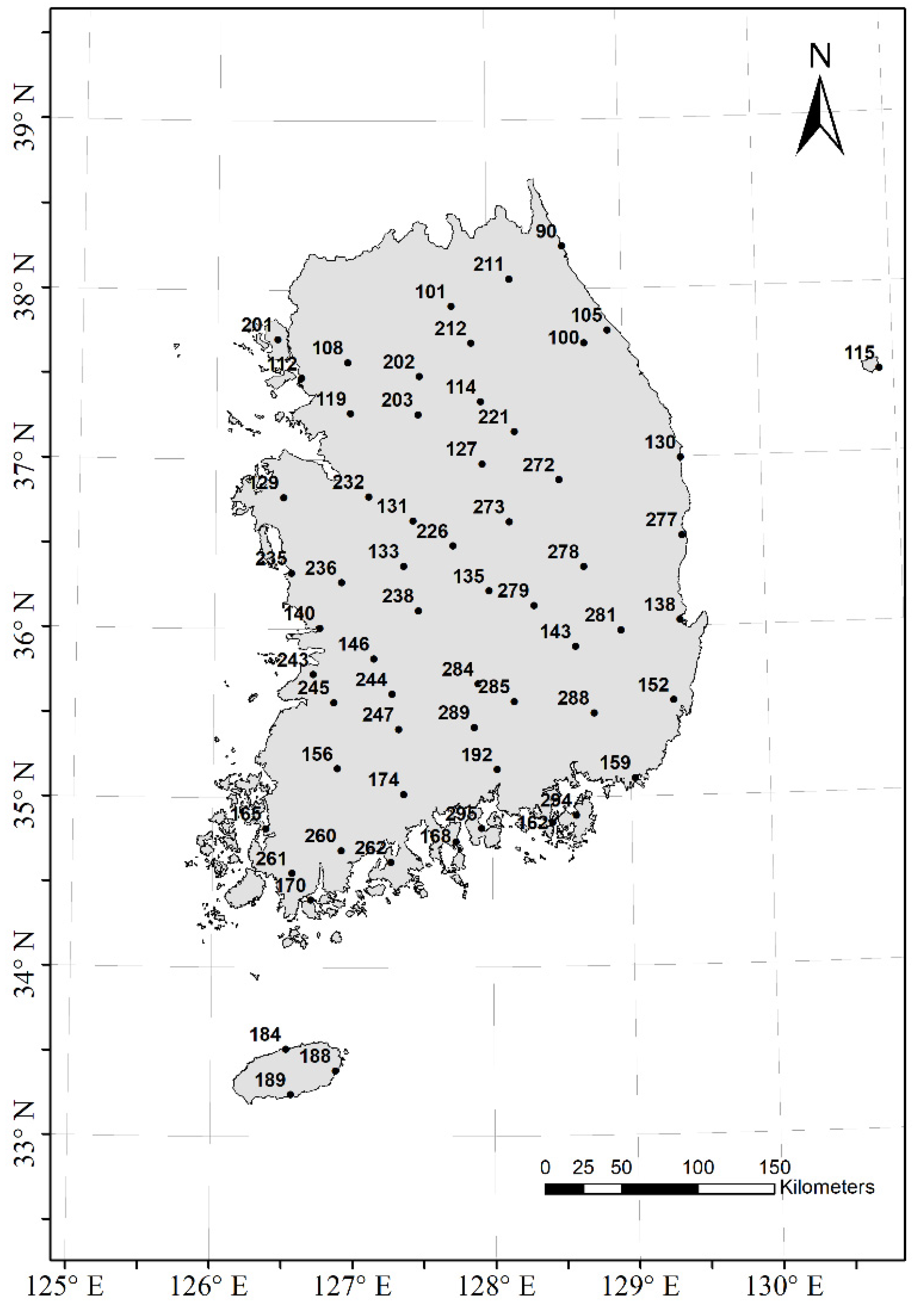
2.1. Annual Maximum Daily Rainfall Data
2.2. Climate Indices
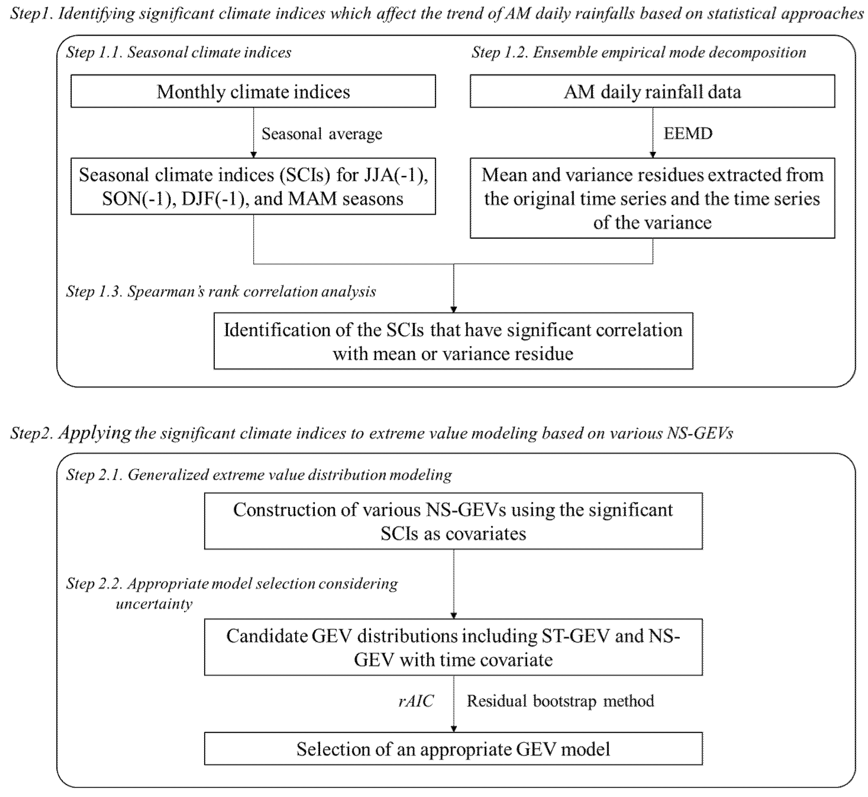
3. Methodology
3.1. Seasonal Climate Indices
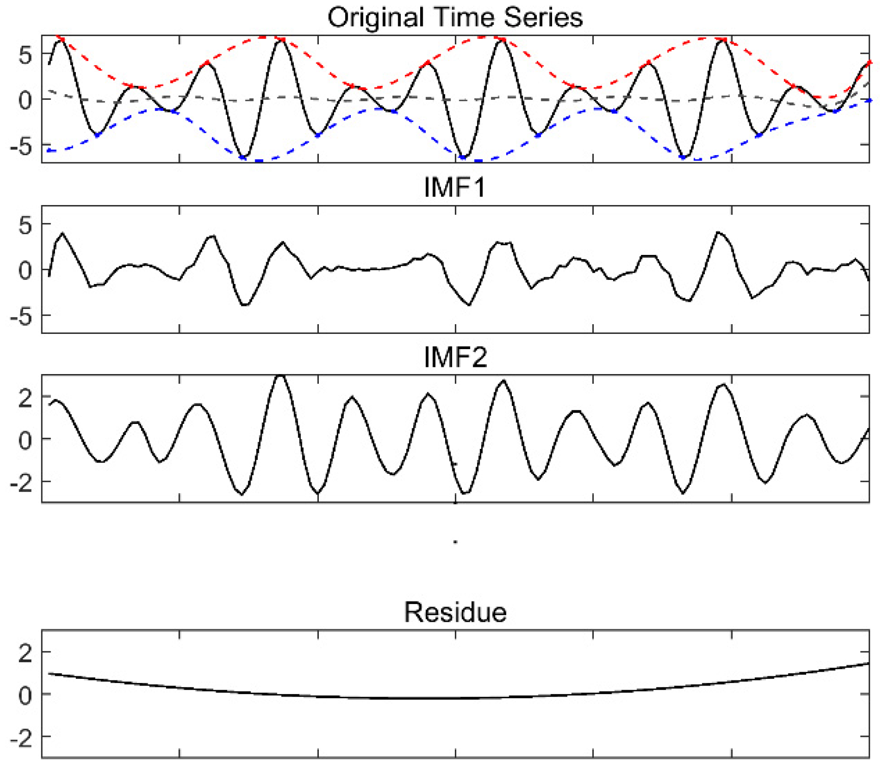
3.2. Ensemble Empirical Mode Decomposition
3.3. Spearman’s Rank Correlation Analysis
3.4. Generalized Extreme Value Distribution Modeling
3.5. Appropriate Model Selection Considering Uncertainty
- For the fitted GEV distribution, transform the AM time series data () into the standardized residuals with no trend () as follows [1]:where the , , and are the location, scale, and shape parameters of the fitted GEV distribution, respectively.
- Obtain a new sample of by resampling residuals with replacement and back-transforming the resampled residuals using Equation (8).
- For back-transformed samples, estimate the T-year quantile at each time (, ) using the same GEV distribution.
- Repeat steps (2)–(3) times and calculate the time-averaged 95% CIs for the T-year quantiles () as follows:where and are the 97.5th and 2.5th percentiles of ordered samples of .
4. Results
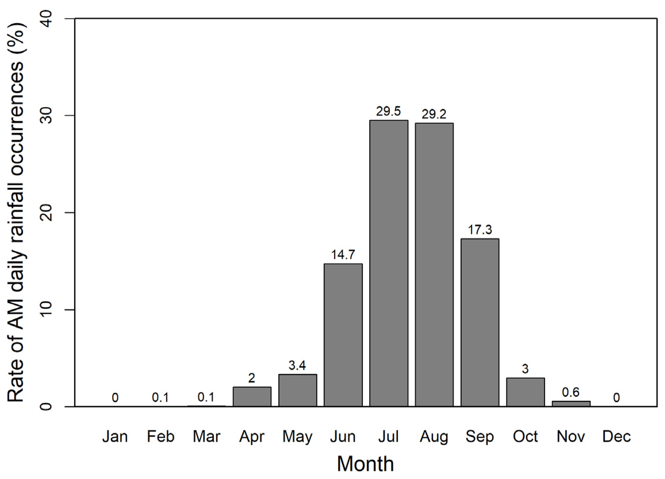
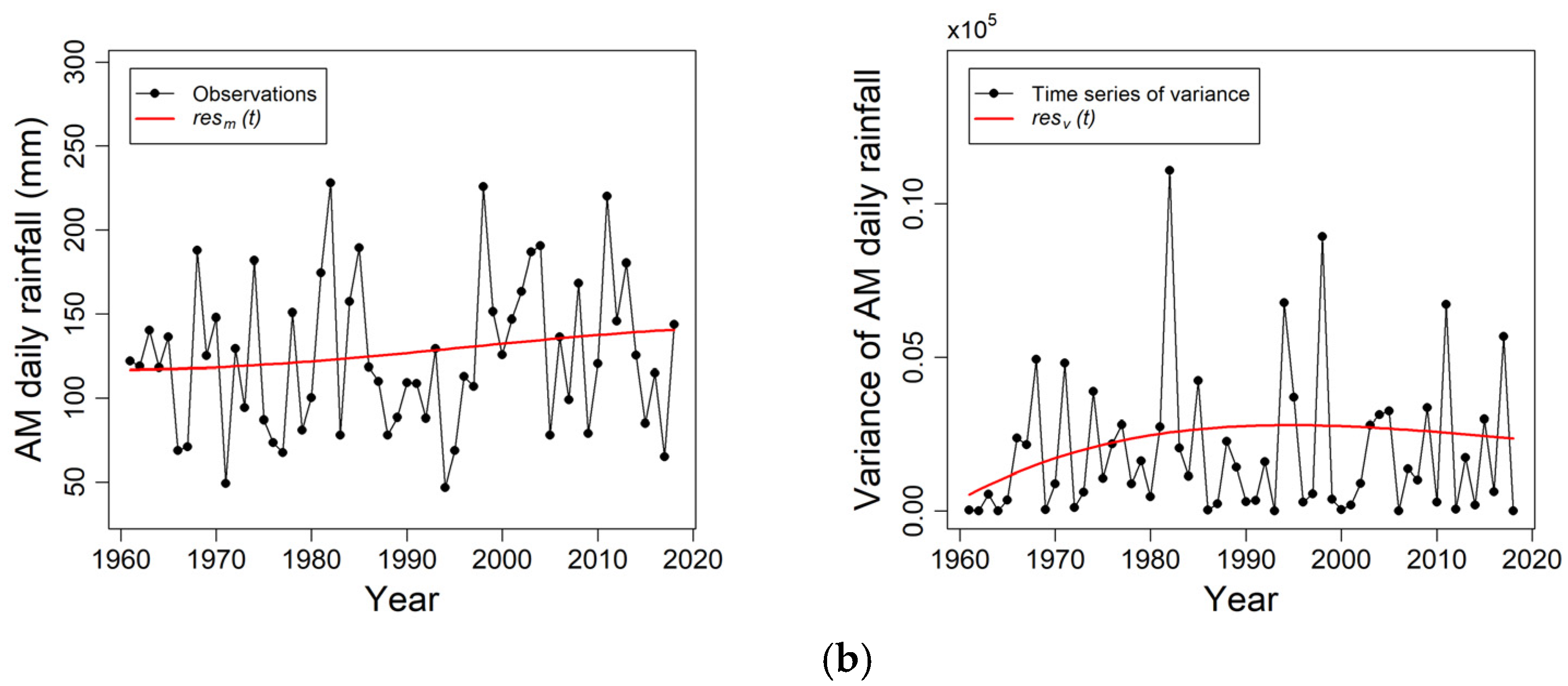
4.1. Mean and Variance Trends of AM Daily Rainfall Extracted Using EEMD
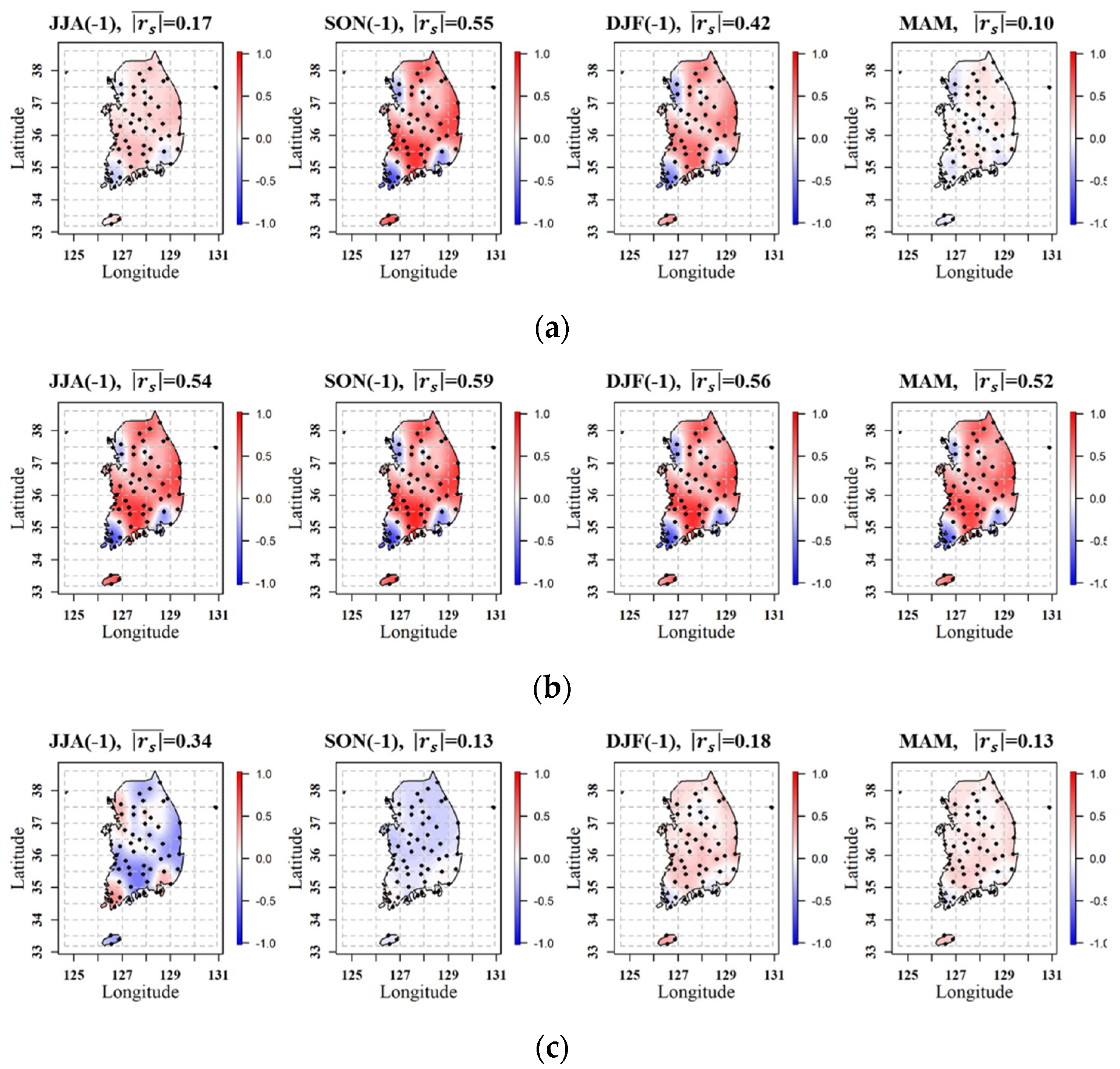
4.2. Significant Seasonal Climate Indices for AM Daily Rainfall over South Korea
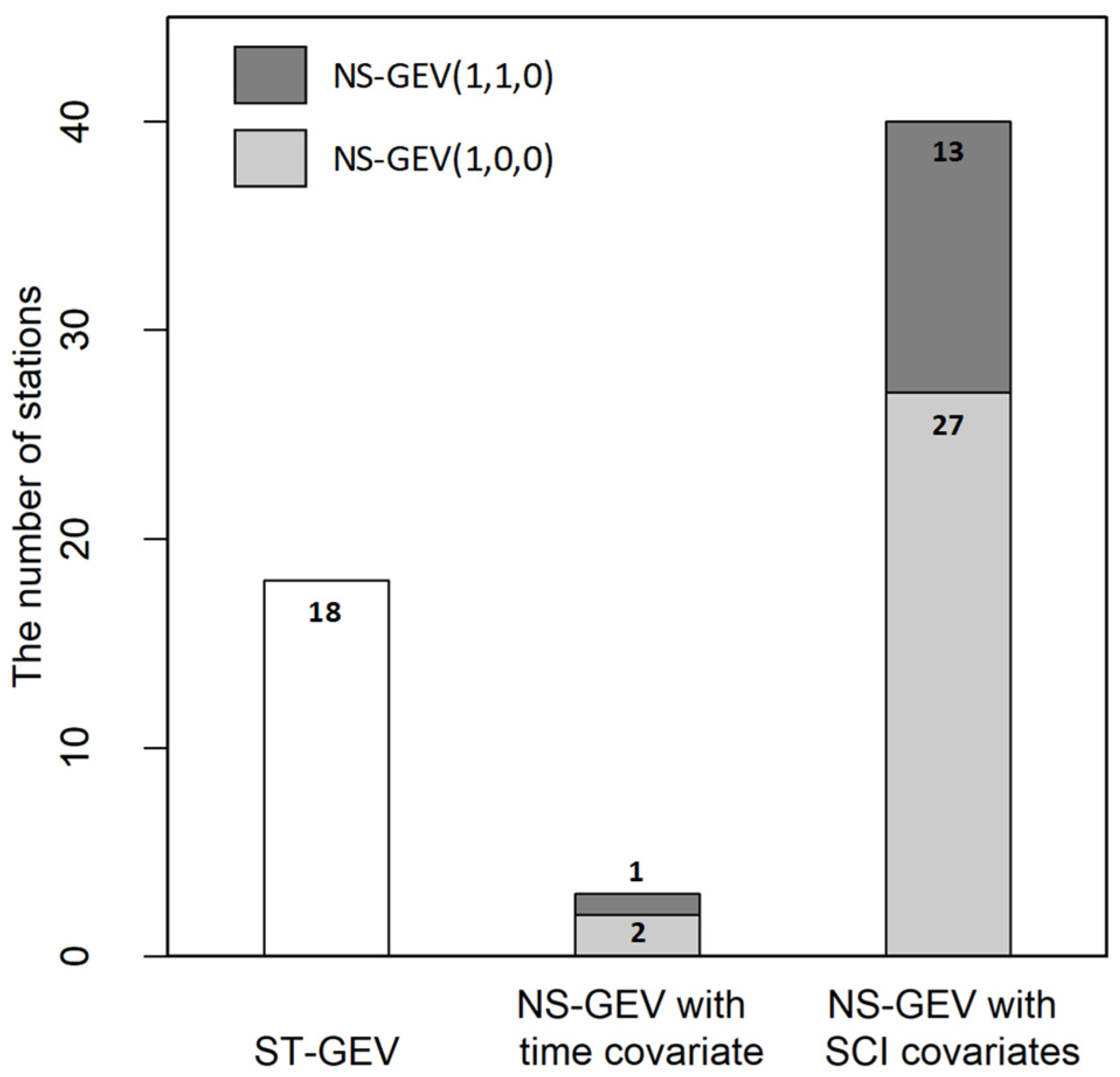
4.3. Appropriate Model Selection Considering Model Fit and Uncertainty
5. Discussions
5.1. Significant Climate Indices for Annual Maximum Rainfall over South Korea
5.2. Consideration of Uncertainty in Model Selection
5.3. Suggestions for Extreme Value Modeling with SCI Covariates
5.4. Limitations of this Study
6. Conclusions
Author Contributions
Funding
Institutional Review Board Statement
Informed Consent Statement
Data Availability Statement
Conflicts of Interest
References
- Coles, S. An Introduction to Statistical Modeling of Extreme Values; Springer: London, UK, 2001. [Google Scholar]
- Koutsoyiannis, D.; Montanari, A. Negligent killing of scientific concepts: The stationarity case. Hydrol. Sci. J. 2015, 60, 1174–1183. [Google Scholar] [CrossRef]
- Serinaldi, F.; Kilsby, C.G. Stationarity is undead: Uncertainty dominates the distribution of extremes. Adv. Water Resour. 2015, 77, 17–36. [Google Scholar] [CrossRef] [Green Version]
- Mondal, A.; Mujumdar, P.P. Hydrologic Extremes Under Climate Change: Non-stationarity and Uncertainty. In Sustainable Water Resources Planning and Management under Climate Change; Kolokytha, E., Oishi, S., Teegavarapu, R.S.V., Eds.; Springer: Singapore, 2017; pp. 39–60. ISBN 978-981-10-2051-3. [Google Scholar]
- Montanari, A.; Koutsoyiannis, D. Modeling and mitigating natural hazards: Stationarity is immortal! Water Resour. Res. 2014, 50, 9748–9756. [Google Scholar] [CrossRef]
- Cheng, L.; Aghakouchak, A. Nonstationary precipitation intensity-duration-frequency curves for infrastructure design in a changing climate. Sci. Rep. 2014, 4, 7093. [Google Scholar] [CrossRef] [PubMed] [Green Version]
- Prosdocimi, I.; Kjeldsen, T.R.; Miller, J.D. Detection and attribution of urbanization effect on flood extremes using nonstationary flood-frequency models. Water Resour. Res. 2015, 51, 4244–4262. [Google Scholar] [CrossRef] [PubMed] [Green Version]
- Vasiliades, L.; Galiatsatou, P.; Loukas, A. Nonstationary Frequency Analysis of Annual Maximum Rainfall Using Climate Covariates. Water Resour. Manag. 2015, 29, 339–358. [Google Scholar] [CrossRef]
- Agilan, V.; Umamahesh, N.V. What are the best covariates for developing non-stationary rainfall Intensity-Duration-Frequency relationship? Adv. Water Resour. 2017, 101, 11–22. [Google Scholar] [CrossRef]
- Salas, J.D.; Obeysekera, J.; Vogel, R.M. Techniques for assessing water infrastructure for nonstationary extreme events: A review. Hydrol. Sci. J. 2018, 63, 325–352. [Google Scholar] [CrossRef]
- Ouarda, T.B.M.J.; El-Adlouni, S. Bayesian nonstationary frequency analysis of hydrological variables. J. Am. Water Resour. Assoc. 2011, 47, 496–505. [Google Scholar] [CrossRef]
- El Adlouni, S.; Ouarda, T.B.M.J.; Zhang, X.; Roy, R.; Bobée, B. Generalized maximum likelihood estimators for the nonstationary generalized extreme value model. Water Resour. Res. 2007, 43, W03410. [Google Scholar] [CrossRef]
- Ganguli, P.; Coulibaly, P. Does nonstationarity in rainfall require nonstationary intensity-duration-frequency curves? Hydrol. Earth Syst. Sci. 2017, 21, 6461–6483. [Google Scholar] [CrossRef] [Green Version]
- Cannon, A.J. A flexible nonlinear modelling framework for nonstationary generalized extreme value analysis in hydroclimatology. Hydrol. Process. 2010, 24, 673–685. [Google Scholar] [CrossRef]
- Zhang, X.; Wang, J.; Zwiers, F.W.; Groisman, P.Y. The Influence of Large-Scale Climate Variability on Winter Maximum Daily Precipitation over North America. J. Clim. 2010, 23, 2902–2915. [Google Scholar] [CrossRef]
- Mondal, A.; Daniel, D. Return levels under nonstationarity: The need to update infrastructure design strategies. J. Hydrol. Eng. 2019, 24, 1–11. [Google Scholar] [CrossRef]
- Agilan, V.; Umamahesh, N.V. Covariate and parameter uncertainty in non-stationary rainfall IDF curve. Int. J. Climatol. 2018, 38, 365–383. [Google Scholar] [CrossRef]
- Kenyon, J.; Hegerl, G.C. Influence of modes of climate variability on global precipitation extremes. J. Clim. 2010, 23, 6248–6262. [Google Scholar] [CrossRef] [Green Version]
- López, J.; Francés, F. Non-stationary flood frequency analysis in continental Spanish rivers, using climate and reservoir indices as external covariates. Hydrol. Earth Syst. Sci. 2013, 17, 3189–3203. [Google Scholar] [CrossRef] [Green Version]
- Casanueva, A.; Rodríguez-Puebla, C.; Frías, M.D.; González-Reviriego, N. Variability of extreme precipitation over Europe and its relationships with teleconnection patterns. Hydrol. Earth Syst. Sci. 2014, 18, 709–725. [Google Scholar] [CrossRef] [Green Version]
- Jha, S.; Das, J.; Goyal, M.K. Low frequency global-scale modes and its influence on rainfall extremes over India: Nonstationary and uncertainty analysis. Int. J. Climatol. 2021, 41, 1873–1888. [Google Scholar] [CrossRef]
- Wu, Z.; Huang, N.E. Ensemble Empirical Mode Decomposition: A Noise-Assisted Data Analysis Method. Adv. Adapt. Data Anal. 2009, 1, 1–41. [Google Scholar] [CrossRef]
- Castino, F.; Bookhagen, B.; Strecker, M.R. Rainfall variability and trends of the past six decades (1950–2014) in the subtropical NW Argentine Andes. Clim. Dyn. 2017, 48, 1049–1067. [Google Scholar] [CrossRef]
- Kim, Y.; Cho, K. Sea level rise around Korea: Analysis of tide gauge station data with the ensemble empirical mode decomposition method. J. Hydro-Environ. Res. 2016, 11, 138–145. [Google Scholar] [CrossRef]
- Zhang, X.; Li, J.; Liu, X.; Chen, Z. Improved EEMD-based standardization method for developing long tree-ring chronologies. J. For. Res. 2019, 31, 2217–2224. [Google Scholar] [CrossRef] [Green Version]
- Chen, P.-C.; Wang, Y.-H.; You, G.J.-Y.; Wei, C.-C. Comparison of methods for non-stationary hydrologic frequency analysis: Case study using annual maximum daily precipitation in Taiwan. J. Hydrol. 2017, 545, 197–211. [Google Scholar] [CrossRef]
- Kim, T.; Shin, J.-Y.; Kim, S.; Heo, J.-H. Identification of relationships between climate indices and long-term precipitation in South Korea using ensemble empirical mode decomposition. J. Hydrol. 2018, 557, 726–739. [Google Scholar] [CrossRef]
- Katz, R.W. Statistical Methods for Nonstationary Extremes. In Extremes in a Changing Climate: Detection, Analysis and Uncertainty; AghaKouchak, A., Easterling, D., Hsu, K., Schubert, S., Sorooshian, S., Eds.; Springer: Dordrecht, The Netherlands, 2013; pp. 15–37. ISBN 978-94-007-4479-0. [Google Scholar]
- Kim, H.; Kim, S.; Shin, H.; Heo, J.-H. Appropriate model selection methods for nonstationary generalized extreme value models. J. Hydrol. 2017, 547, 557–574. [Google Scholar] [CrossRef]
- Strupczewski, W.G.; Singh, V.P.; Feluch, W. Non-stationarity approach to at-site flood frequency modeling I. Maximum likelihood estimation. J. Hydrol. 2001, 248, 123–142. [Google Scholar] [CrossRef]
- Thiombiano, A.N.; St-Hilaire, A.; El Adlouni, S.E.; Ouarda, T.B.M.J. Nonlinear response of precipitation to climate indices using a non-stationary Poisson-generalized Pareto model: Case study of southeastern Canada. Int. J. Climatol. 2018, 38, e875–e888. [Google Scholar] [CrossRef]
- Villarini, G.; Smith, J.A.; Ntelekos, A.A.; Schwarz, U. Annual maximum and peaks-over-threshold analyses of daily rainfall accumulations for Austria. J. Geophys. Res. Atmos. 2011, 116, D05103. [Google Scholar] [CrossRef]
- Villarini, G.; Smith, J.A.; Serinaldi, F.; Ntelekos, A.A.; Schwarz, U. Analyses of extreme flooding in Austria over the period 1951–2006. Int. J. Climatol. 2012, 32, 1178–1192. [Google Scholar] [CrossRef]
- Cooley, D. Return Periods and Return Levels Under Climate Change. In Extremes in a Changing Climate: Detection, Analysis and Uncertainty; AghaKouchak, A., Easterling, D., Hsu, K., Schubert, S., Sorooshian, S., Eds.; Springer: Dordrecht, The Netherlands, 2013; pp. 97–114. ISBN 978-94-007-4479-0. [Google Scholar]
- Hesarkazzazi, S.; Arabzadeh, R.; Hajibabaei, M.; Rauch, W.; Kjeldsen, T.R.; Prosdocimi, I.; Castellarin, A.; Sitzenfrei, R. Stationary vs. non-stationary modelling of flood frequency distribution across northwest England. Hydrol. Sci. J. 2021, 66, 729–744. [Google Scholar] [CrossRef]
- Ouarda, T.B.M.J.; Charron, C.; St-Hilaire, A. Uncertainty of stationary and nonstationary models for rainfall frequency analysis. Int. J. Climatol. 2020, 40, 2373–2392. [Google Scholar] [CrossRef]
- O’Brien, N.L.; Burn, D.H. A nonstationary index-flood technique for estimating extreme quantiles for annual maximum streamflow. J. Hydrol. 2014, 519, 2040–2048. [Google Scholar] [CrossRef]
- Tramblay, Y.; Neppel, L.; Carreau, J.; Najib, K. Non-stationary frequency analysis of heavy rainfall events in southern France. Hydrol. Sci. J. 2013, 58, 280–294. [Google Scholar] [CrossRef]
- Silva, A.T.; Naghettini, M.; Portela, M.M. On some aspects of peaks-over-threshold modeling of floods under nonstationarity using climate covariates. Stoch. Environ. Res. Risk Assess. 2016, 30, 207–224. [Google Scholar] [CrossRef]
- Obeysekera, J.; Salas, J.D. Quantifying the Uncertainty of Design Floods under Nonstationary Conditions. J. Hydrol. Eng. 2014, 19, 1438–1446. [Google Scholar] [CrossRef]
- Hu, Y.; Liang, Z.; Chen, X.; Liu, Y.; Wang, H.; Yang, J.; Wang, J.; Li, B. Estimation of design flood using EWT and ENE metrics and uncertainty analysis under non-stationary conditions. Stoch. Environ. Res. Risk Assess. 2017, 31, 2617–2626. [Google Scholar] [CrossRef]
- Ng, J.L.; Abd Aziz, S.; Huang, Y.F.; Mirzaei, M.; Wayayok, A.; Rowshon, M.K. Uncertainty analysis of rainfall depth duration frequency curves using the bootstrap resampling technique. J. Earth Syst. Sci. 2019, 128, 113. [Google Scholar] [CrossRef] [Green Version]
- Ossandón, Á.; Rajagopalan, B.; Kleiber, W. Spatial-temporal multivariate semi-Bayesian hierarchical framework for extreme precipitation frequency analysis. J. Hydrol. 2021, 600, 126499. [Google Scholar] [CrossRef]
- Seo, Y.A.; Lee, Y.; Park, J.S.; Kim, M.K.; Cho, C.; Baek, H.J. Assessing changes in observed and future projected precipitation extremes in South Korea. Int. J. Climatol. 2015, 35, 1069–1078. [Google Scholar] [CrossRef]
- Wi, S.; Valdés, J.B.; Steinschneider, S.; Kim, T.-W. Non-stationary frequency analysis of extreme precipitation in South Korea using peaks-over-threshold and annual maxima. Stoch. Environ. Res. Risk Assess. 2016, 30, 583–606. [Google Scholar] [CrossRef]
- Sung, J.H.; Kim, Y.O.; Jeon, J.J. Application of distribution-free nonstationary regional frequency analysis based on L-moments. Theor. Appl. Climatol. 2018, 133, 1219–1233. [Google Scholar] [CrossRef]
- Huang, N.E.; Shen, Z.; Long, S.R.; Wu, M.C.; Snin, H.H.; Zheng, Q.; Yen, N.C.; Tung, C.C.; Liu, H.H. The empirical mode decomposition and the Hubert spectrum for nonlinear and non-stationary time series analysis. Proc. R. Soc. A Math. Phys. Eng. Sci. 1998, 454, 903–995. [Google Scholar] [CrossRef]
- King, A.D.; Klingaman, N.P.; Alexander, L.V.; Donat, M.G.; Jourdain, N.C.; Maher, P. Extreme Rainfall Variability in Australia: Patterns, Drivers, and Predictability. J. Clim. 2014, 27, 6035–6050. [Google Scholar] [CrossRef] [Green Version]
- Dehghan, Z.; Eslamian, S.S.; Modarres, R. Spatial clustering of maximum 24-h rainfall over Urmia Lake Basin by new weighting approaches. Int. J. Climatol. 2018, 38, 2298–2313. [Google Scholar] [CrossRef]
- Ratner, B. The correlation coefficient: Its values range between +1/−1, or do they? J. Target. Meas. Anal. Mark. 2009, 17, 139–142. [Google Scholar] [CrossRef] [Green Version]
- Corder, G.W.; Foreman, D.I. Nonparametric Statistics for Non-Statisticians: A Step-by-Step Approach; Wiley: Hoboken, NJ, USA, 2009; ISBN 9780470454619. [Google Scholar]
- Hinkle, D.E.; Wiersma, W.; Jurs, S.G. Applied Statistics for the Behavioral Sciences, 5th ed.; Houghton Mifflin: Boston, MA, USA, 2003; ISBN 9780618124053. [Google Scholar]
- Burnham, K.P.; Anderson, D.R. Multimodel inference: Understanding AIC and BIC in model selection. Sociol. Methods Res. 2004, 33, 261–304. [Google Scholar] [CrossRef]
- Kharin, V.V.; Zwiers, F.W. Estimating extremes in transient climate change simulations. J. Clim. 2005, 18, 1156–1173. [Google Scholar] [CrossRef]
- Khaliq, M.N.; Ouarda, T.B.M.J.; Ondo, J.-C.; Gachon, P.; Bobée, B. Frequency analysis of a sequence of dependent and/or non-stationary hydro-meteorological observations: A review. J. Hydrol. 2006, 329, 534–552. [Google Scholar] [CrossRef]
- Hanel, M.; Buishand, T.A.; Ferro, C.A.T. A nonstationary index flood model for precipitation extremes in transient regional climate model simulations. J. Geophys. Res. Atmos. 2009, 114, D15107. [Google Scholar] [CrossRef]
- Knight, J.R.; Allan, R.J.; Folland, C.K.; Vellinga, M.; Mann, M.E. A signature of persistent natural thermohaline circulation cycles in observed climate. Geophys. Res. Lett. 2005, 32, L20708. [Google Scholar] [CrossRef] [Green Version]
- Lu, R.; Dong, B.; Ding, H. Impact of the Atlantic Multidecadal Oscillation on the Asian summer monsoon. Geophys. Res. Lett. 2006, 33, 1–5. [Google Scholar] [CrossRef] [Green Version]
- Li, S.; Bates, G.T. Influence of the Atlantic Multidecadal Oscillation on the winter climate of East China. Adv. Atmos. Sci. 2007, 24, 126–135. [Google Scholar] [CrossRef]
- Si, D.; Ding, Y. Oceanic forcings of the interdecadal variability in east Asian summer rainfall. J. Clim. 2016, 29, 7633–7649. [Google Scholar] [CrossRef]
- Li, Y.; Ding, Y.; Li, W. Interdecadal variability of the Afro-Asian summer monsoon system. Adv. Atmos. Sci. 2017, 34, 833–846. [Google Scholar] [CrossRef]
- Vimont, D.J.; Kossin, J.P. The Atlantic Meridional Mode and hurricane activity. Geophys. Res. Lett. 2007, 34, 1–5. [Google Scholar] [CrossRef] [Green Version]
- van Loon, H.; Rogers, J.C. The Seesaw in Winter Temperatures between Greenland and Northern Europe. Part I: General Description. Mon. Weather Rev. 1978, 106, 296–310. [Google Scholar] [CrossRef] [Green Version]
- Liu, X.; Yin, Z.-Y. Spatial and Temporal Variation of Summer Precipitation over the Eastern Tibetan Plateau and the North Atlantic Oscillation. J. Clim. 2001, 14, 2896–2909. [Google Scholar] [CrossRef] [Green Version]
- Gu, W.; Li, C.; Li, W.; Zhou, W.; Chan, J.C.L. Interdecadal unstationary relationship between NAO and east China’s summer precipitation patterns. Geophys. Res. Lett. 2009, 36, L13702. [Google Scholar] [CrossRef]
- Wu, Z.; Wang, B.; Li, J.; Jin, F.-F. An empirical seasonal prediction model of the east Asian summer monsoon using ENSO and NAO. J. Geophys. Res. Atmos. 2009, 114, D18120. [Google Scholar] [CrossRef]
- Jin, D.; Guan, Z. Summer Rainfall Seesaw between Hetao and the Middle and Lower Reaches of the Yangtze River and Its Relationship with the North Atlantic Oscillation. J. Clim. 2017, 30, 6629–6643. [Google Scholar] [CrossRef]
- Linderholm, H.W.; Ou, T.; Jeong, J.H.; Folland, C.K.; Gong, D.; Liu, H.; Liu, Y.; Chen, D. Interannual teleconnections between the summer North Atlantic Oscillation and the East Asian summer monsoon. J. Geophys. Res. Atmos. 2011, 116, 1–13. [Google Scholar] [CrossRef]
- Sun, J.; Wang, H. Changes of the connection between the summer North Atlantic Oscillation and the East Asian summer rainfall. J. Geophys. Res. Atmos. 2012, 117, 1–12. [Google Scholar] [CrossRef]
- Wang, Z.; Yang, S.; Lau, N.C.; Duan, A. Teleconnection between summer NAO and East China rainfall variations: A bridge effect of the Tibetan Plateau. J. Clim. 2018, 31, 6433–6444. [Google Scholar] [CrossRef]
- Merz, B.; Vorogushyn, S.; Uhlemann, S.; Delgado, J.; Hundecha, Y. HESS Opinions More efforts and scientific rigour are needed to attribute trends in flood time series. Hydrol. Earth Syst. Sci. 2012, 16, 1379–1387. [Google Scholar] [CrossRef] [Green Version]
- Eden, J.M.; Wolter, K.; Otto, F.E.L.; Jan van Oldenborgh, G. Multi-method attribution analysis of extreme precipitation in Boulder, Colorado. Environ. Res. Lett. 2016, 11, 124009. [Google Scholar] [CrossRef] [Green Version]
- Ministry of Environment. Standard Guidelines for Design Flood Estimation; Ministry of Environment: Sejong City, Korea, 2019.
- Zaifoglu, H.; Akintug, B.; Yanmaz, A.M. Regional frequency analysis of precipitation using time series clustering approaches. J. Hydrol. Eng. 2018, 23, 1–13. [Google Scholar] [CrossRef]
- Kyselý, J.; Picek, J. Regional growth curves and improved design value estimates of extreme precipitation events in the Czech Republic. Clim. Res. 2007, 33, 243–255. [Google Scholar] [CrossRef]
- Wang, Z.; Zeng, Z.; Lai, C.; Lin, W.; Wu, X.; Chen, X. A regional frequency analysis of precipitation extremes in Mainland China with fuzzy c-means and L-moments approaches. Int. J. Climatol. 2017, 37, 429–444. [Google Scholar] [CrossRef]
- Kim, S.; Nam, W.; Ahn, H.; Kim, T.; Heo, J.-H. Comparison of nonstationary generalized logistic models based on Monte Carlo simulation. Proc. IAHS 2015, 371, 65–68. [Google Scholar] [CrossRef] [Green Version]


| Code | Name | Longitude | Latitude | Record Length (year) | Code | Name | Longitude | Latitude | Record Length (year) |
|---|---|---|---|---|---|---|---|---|---|
| 90 | Sokcho | 128.6 | 38.3 | 50 | 201 | Ganghwa | 126.4 | 37.7 | 45 |
| 100 | Daegwallyeong | 128.7 | 37.7 | 46 | 202 | Yangpyeong | 127.5 | 37.5 | 45 |
| 101 | Chuncheon | 127.7 | 37.9 | 52 | 203 | Icheon | 127.5 | 37.3 | 45 |
| 105 | Gangneung | 128.9 | 37.8 | 57 | 211 | Inje | 128.2 | 38.1 | 45 |
| 108 | Seoul | 127.0 | 37.6 | 57 | 212 | Hongcheon | 127.9 | 37.7 | 45 |
| 112 | Incheon | 126.6 | 37.5 | 57 | 221 | Jecheon | 128.2 | 37.2 | 45 |
| 114 | Wonju | 127.9 | 37.3 | 45 | 226 | Boeun | 127.7 | 36.5 | 45 |
| 115 | Ulleungdo | 130.9 | 37.5 | 57 | 232 | Cheonan | 127.1 | 36.8 | 45 |
| 119 | Suwon | 127.0 | 37.3 | 54 | 235 | Boryeong | 126.6 | 36.3 | 45 |
| 127 | Chungju | 128.0 | 37.0 | 45 | 236 | Buyeo | 126.9 | 36.3 | 45 |
| 129 | Seosan | 126.5 | 36.8 | 50 | 238 | Geumsan | 127.5 | 36.1 | 45 |
| 130 | Uljin | 129.4 | 37.0 | 46 | 243 | Buan | 126.7 | 35.7 | 45 |
| 131 | Cheongju | 127.4 | 36.6 | 51 | 244 | Imsil | 127.3 | 35.6 | 45 |
| 133 | Daejeon | 127.4 | 36.4 | 49 | 245 | Jeongeup | 126.9 | 35.6 | 45 |
| 135 | Chupungnyeong | 128.0 | 36.2 | 57 | 247 | Namwon | 127.3 | 35.4 | 45 |
| 138 | Pohang | 129.4 | 36.0 | 57 | 260 | Jangheung | 126.9 | 34.7 | 45 |
| 140 | Gunsan | 126.8 | 36.0 | 50 | 261 | Haenam | 126.6 | 34.6 | 45 |
| 143 | Daegu | 128.6 | 35.9 | 57 | 262 | Goheung | 127.3 | 34.6 | 45 |
| 146 | Jeonju | 127.2 | 35.8 | 57 | 272 | Yeongju | 128.5 | 36.9 | 45 |
| 152 | Ulsan | 129.3 | 35.6 | 57 | 273 | Mungyeong | 128.1 | 36.6 | 45 |
| 156 | Gwangju | 126.9 | 35.2 | 57 | 277 | Yeongdeok | 129.4 | 36.5 | 45 |
| 159 | Busan | 129.0 | 35.1 | 57 | 278 | Uiseong | 128.7 | 36.4 | 45 |
| 162 | Tongyeong | 128.4 | 34.8 | 50 | 279 | Gumi | 128.3 | 36.1 | 45 |
| 165 | Mokpo | 126.4 | 34.8 | 57 | 281 | Yeongcheon | 129.0 | 36.0 | 45 |
| 168 | Yoesu | 127.7 | 34.7 | 57 | 284 | Geochang | 127.9 | 35.7 | 45 |
| 170 | Wando | 126.7 | 34.4 | 45 | 285 | Hapcheon | 128.2 | 35.6 | 45 |
| 174 | Suncheon | 127.4 | 35.0 | 45 | 288 | Miryang | 128.7 | 35.5 | 45 |
| 184 | Jeju | 126.5 | 33.5 | 57 | 289 | Sancheong | 127.9 | 35.4 | 45 |
| 188 | Seongsan | 126.9 | 33.4 | 45 | 294 | Geoje | 128.6 | 34.9 | 45 |
| 189 | Seogwipo | 126.6 | 33.2 | 57 | 295 | Namhae | 127.9 | 34.8 | 45 |
| 192 | Jinju | 128.0 | 35.2 | 49 |
| Abbreviation | JJA(−1) | SON(−1) | DJF(−1) | MAM |
|---|---|---|---|---|
| Description | Averaged from Jun. to Aug. (summer season) in the previous year of AM rainfall occurrence | Averaged from Sep. to Nov. (fall season) in the previous year of AM rainfall occurrence | Averaged from Dec. to Feb. (winter season) in the previous year of AM rainfall occurrence | Averaged from Mar. to May (spring season) in the year of AM rainfall occurrence |
| Climate Index | Season | |||
|---|---|---|---|---|
| JJA(−1) | SON(−1) | DJF(−1) | MAM | |
| AMM | - | 77% | 67.2% | - |
| AMO | 75.4% | 77% | 77% | 77% |
| AO | - | - | - | - |
| NAO | 57.4% | - | 13.1% | - |
| NINO12 | 4.9% | - | - | - |
| NINO4 | - | - | - | - |
| NINO34 | 19.7% | - | - | - |
| NP | - | - | - | 6.6% |
| PDO | 9.8% | - | - | 9.8% |
| PMM | - | - | - | - |
| PNA | - | - | - | 8.2% |
| SOI | - | - | - | - |
| Climate Index | Season | |||
|---|---|---|---|---|
| JJA(−1) | SON(−1) | DJF(−1) | MAM | |
| AMM | - | 75.4% | 68.9% | - |
| AMO | 72.1% | 82% | 80.3% | 73.8% |
| AO | - | - | - | - |
| NAO | 68.9% | - | 13.1% | - |
| NINO12 | 3.3% | - | - | - |
| NINO4 | - | - | - | - |
| NINO34 | 14.8% | - | - | - |
| NP | - | - | - | 3.3% |
| PDO | 13.1% | - | - | 11.5% |
| PMM | - | - | - | - |
| PNA | - | - | - | 8.2% |
| SOI | - | - | - | - |
| Distribution Type | GEV Parameters | The Number of Models | ||
|---|---|---|---|---|
| Location, | Scale, | Shape, | ||
| ST-GEV | 1 | |||
| NS-GEV(1,0,0) with time covariate | 1 | |||
| NS-GEV(1,1,0) with time covariate | 1 | |||
| NS-GEV(1,0,0) with SCI covariates |
| 7 | ||
| NS-GEV(1,1,0) with SCI covariates |
|
| 49 | |
| Distribution Type | rAIC Value | GEV Parameters | Uncertainty, | ||
|---|---|---|---|---|---|
| Location, | Scale, | Shape, | |||
| NS-GEV(1,0,0) with SCI covariates | 0 | 102.2 | |||
| NS-GEV(1,0,0) with SCI covariates | 0.24 | 88.8 | |||
| NS-GEV(1,1,0) with SCI covariates | 1.69 | 116.6 | |||
| ST-GEV | 1.74 | 109.5 | |||
| NS-GEV(1,1,0) with SCI covariates | 1.80 | 121.3 | |||
| NS-GEV(1,0,0) with SCI covariates | 1.81 | 103.1 | |||
| NS-GEV(1,1,0) with SCI covariates | 1.81 | 109.7 | |||
| NS-GEV(1,0,0) with SCI covariates | 1.82 | 108.2 | |||
| NS-GEV(1,0,0) with SCI covariates | 1.95 | 115.6 | |||
| NS-GEV(1,1,0) with SCI covariates | 1.95 | 124.7 | |||
Publisher’s Note: MDPI stays neutral with regard to jurisdictional claims in published maps and institutional affiliations. |
© 2022 by the authors. Licensee MDPI, Basel, Switzerland. This article is an open access article distributed under the terms and conditions of the Creative Commons Attribution (CC BY) license (https://creativecommons.org/licenses/by/4.0/).
Share and Cite
Kim, H.; Kim, T.; Shin, J.-Y.; Heo, J.-H. Improvement of Extreme Value Modeling for Extreme Rainfall Using Large-Scale Climate Modes and Considering Model Uncertainty. Water 2022, 14, 478. https://doi.org/10.3390/w14030478
Kim H, Kim T, Shin J-Y, Heo J-H. Improvement of Extreme Value Modeling for Extreme Rainfall Using Large-Scale Climate Modes and Considering Model Uncertainty. Water. 2022; 14(3):478. https://doi.org/10.3390/w14030478
Chicago/Turabian StyleKim, Hanbeen, Taereem Kim, Ju-Young Shin, and Jun-Haeng Heo. 2022. "Improvement of Extreme Value Modeling for Extreme Rainfall Using Large-Scale Climate Modes and Considering Model Uncertainty" Water 14, no. 3: 478. https://doi.org/10.3390/w14030478
APA StyleKim, H., Kim, T., Shin, J.-Y., & Heo, J.-H. (2022). Improvement of Extreme Value Modeling for Extreme Rainfall Using Large-Scale Climate Modes and Considering Model Uncertainty. Water, 14(3), 478. https://doi.org/10.3390/w14030478