
Simulation of Wave Time Series with a Vector Autoregressive Method


Abstract
:1. Introduction
2. Methodology
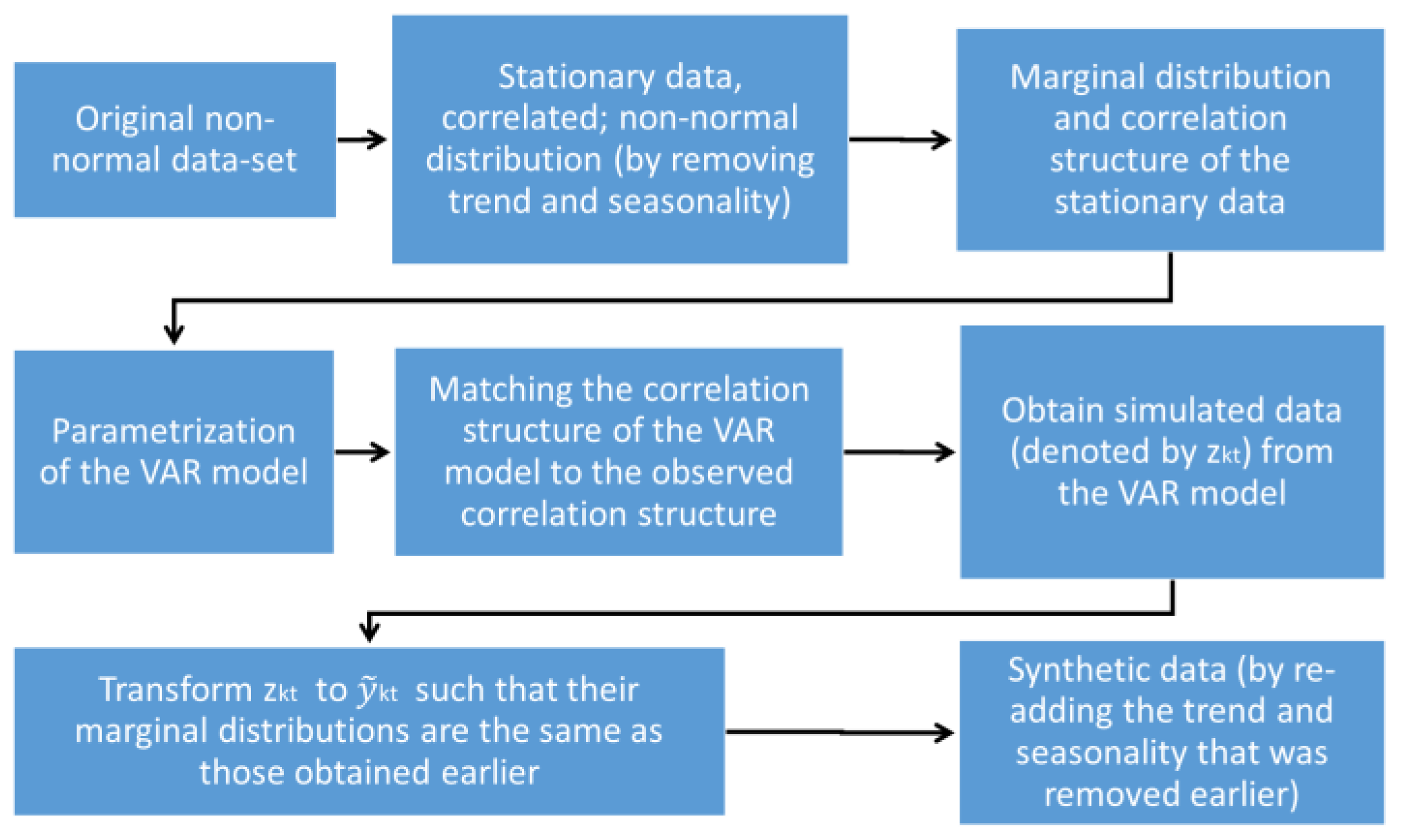
2.1. Outline
2.2. Detailed Methodology
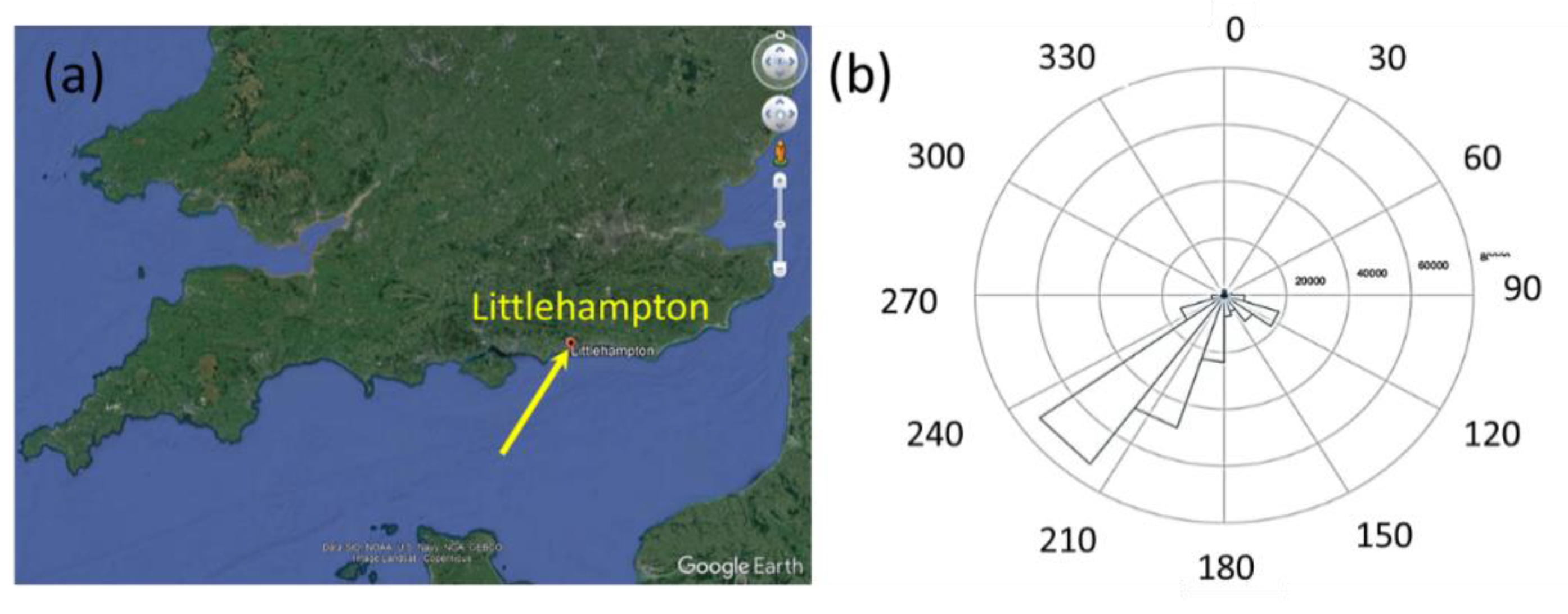
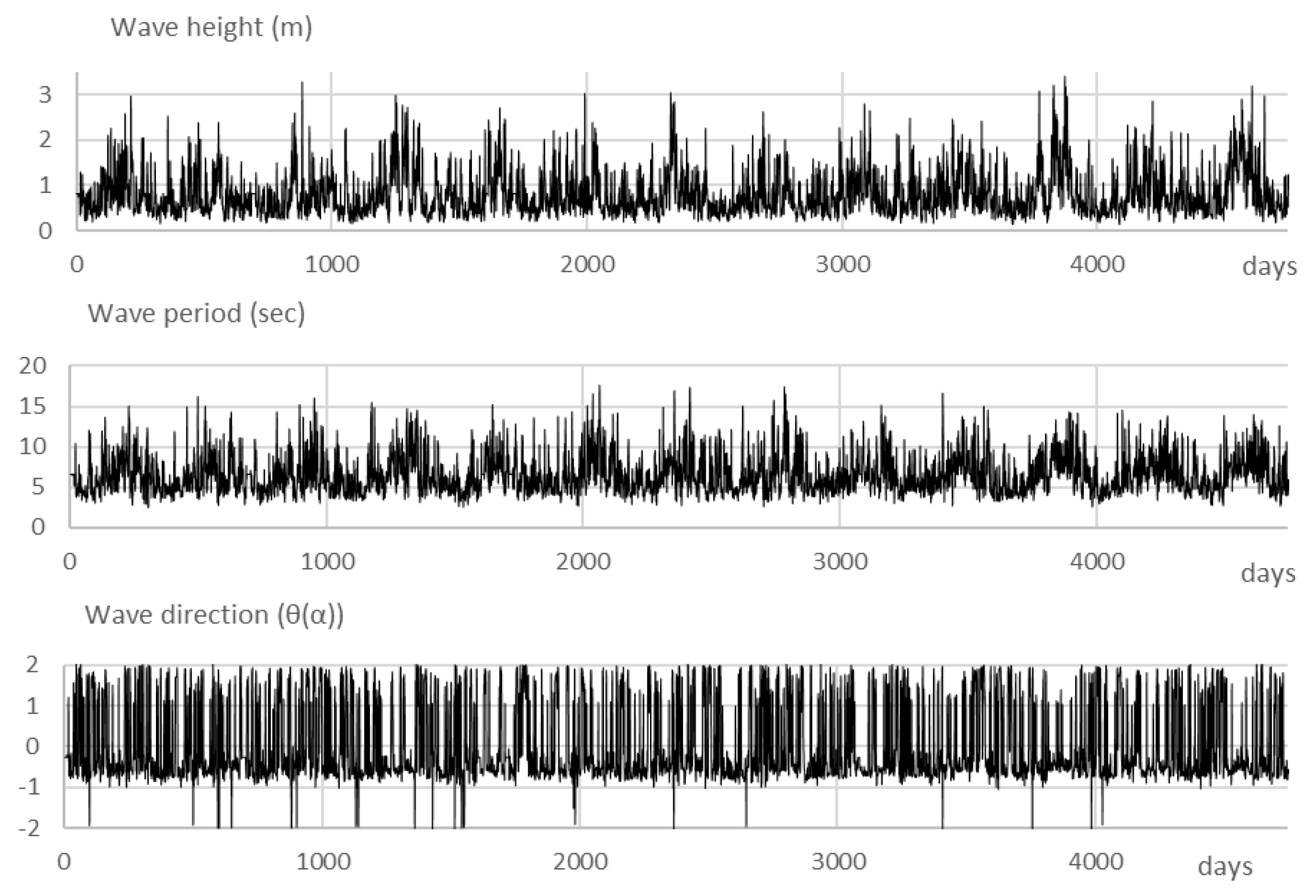
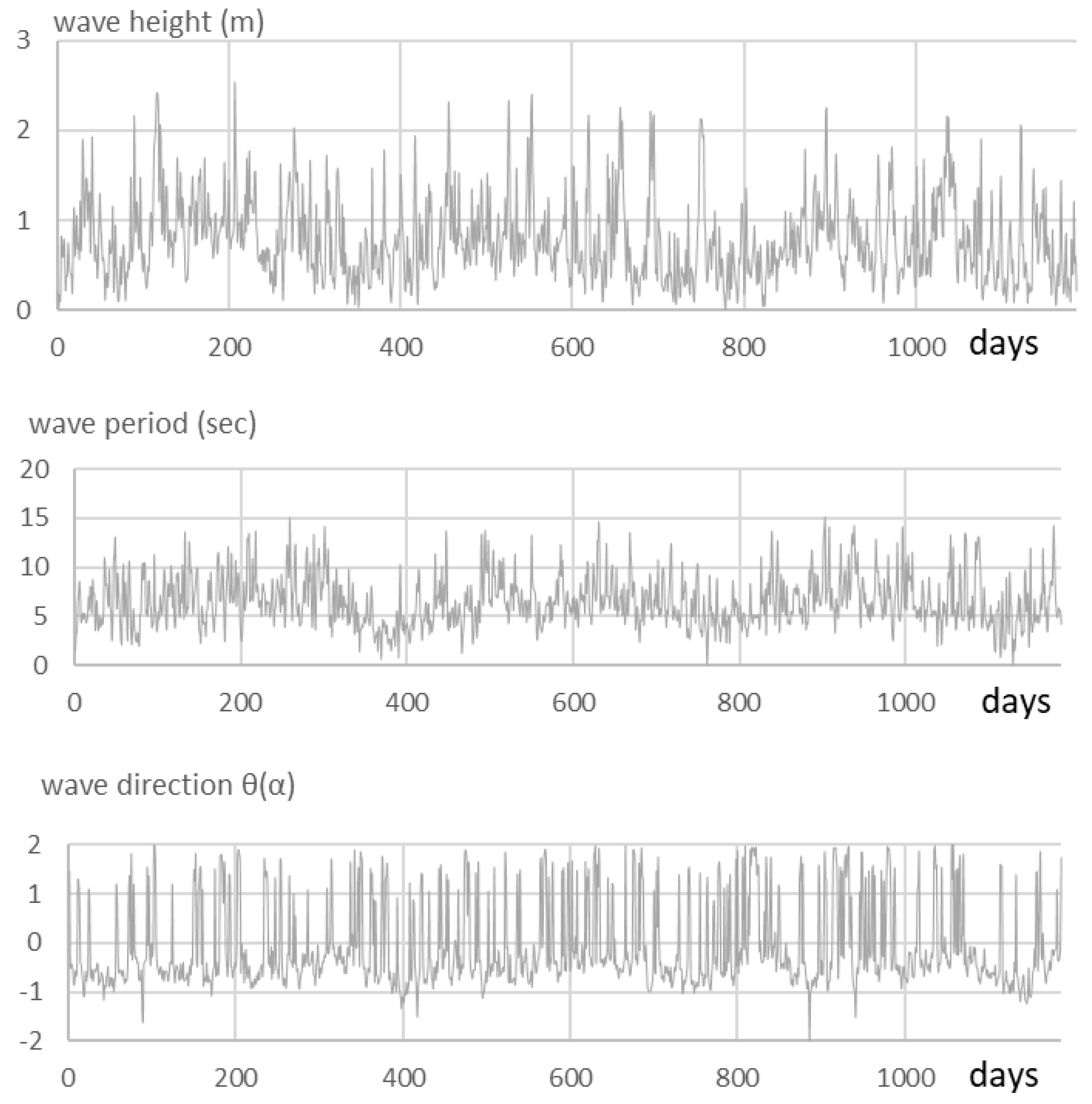
3. Case-Study and Data Processing
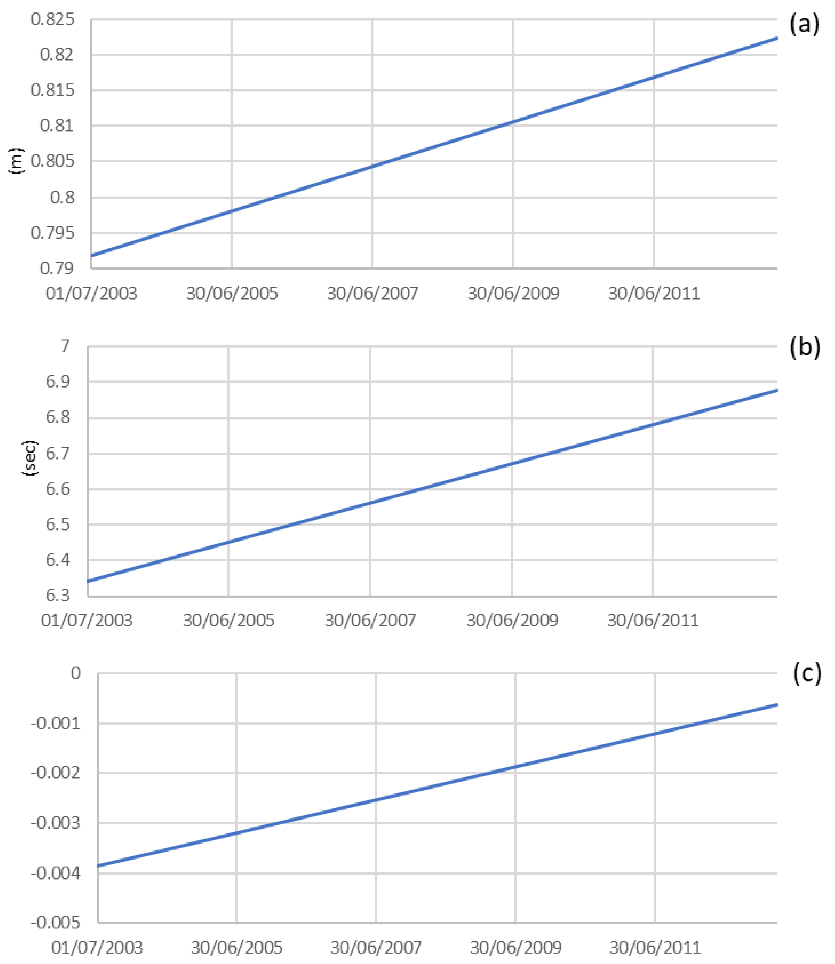
3.1. Detrending
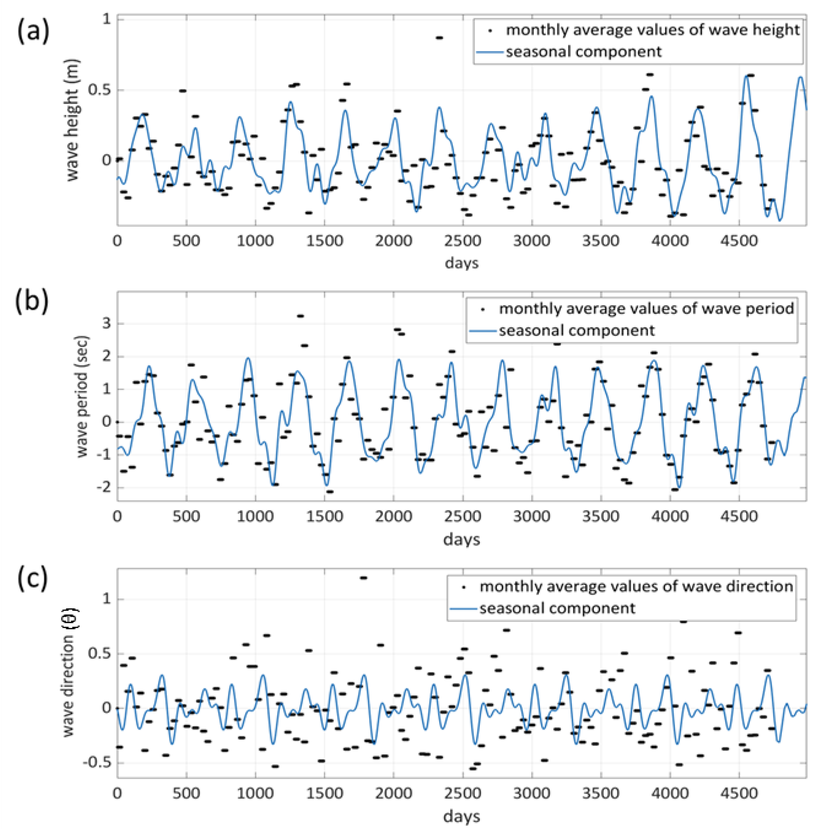
3.2. Seasonality
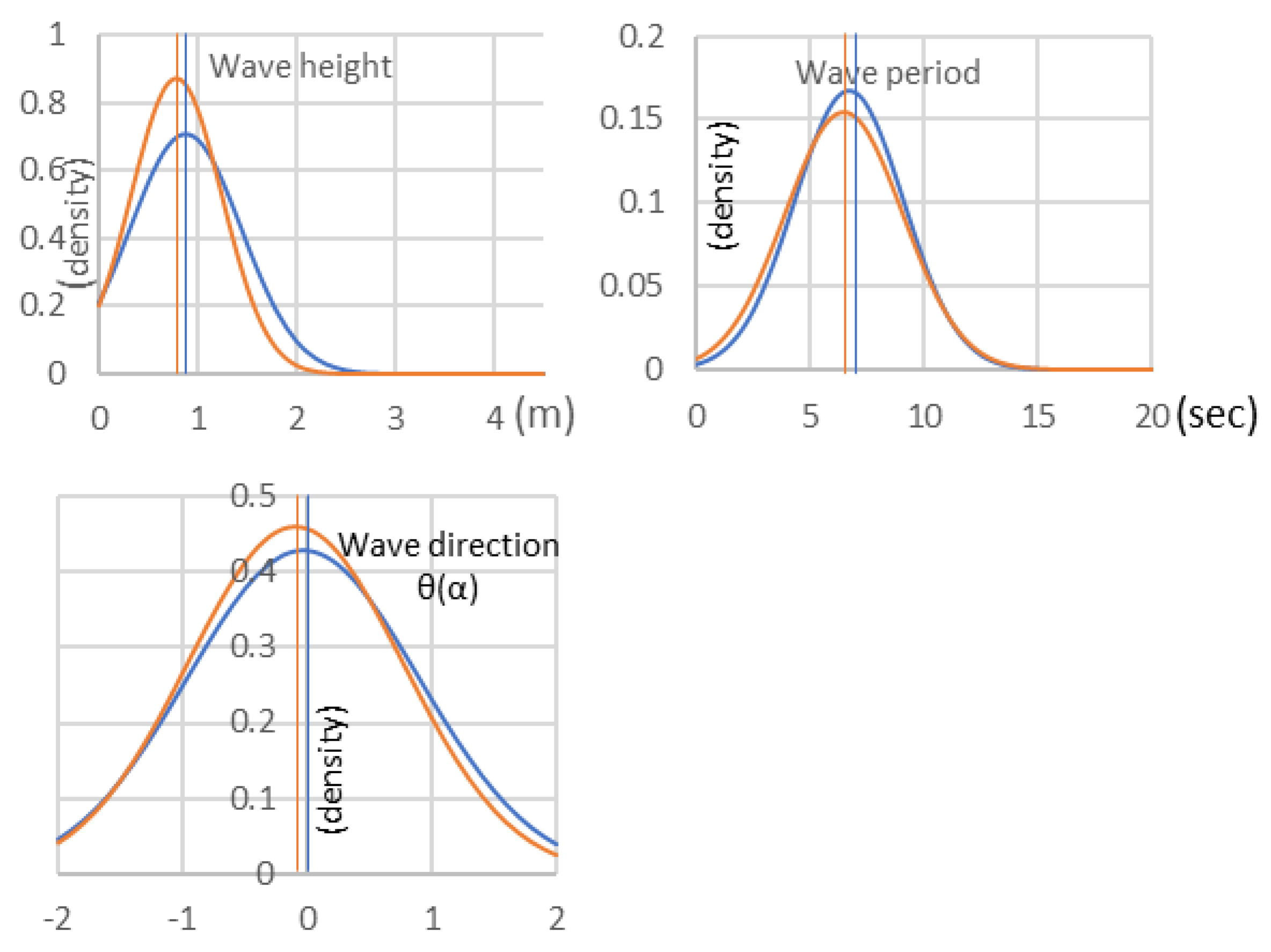
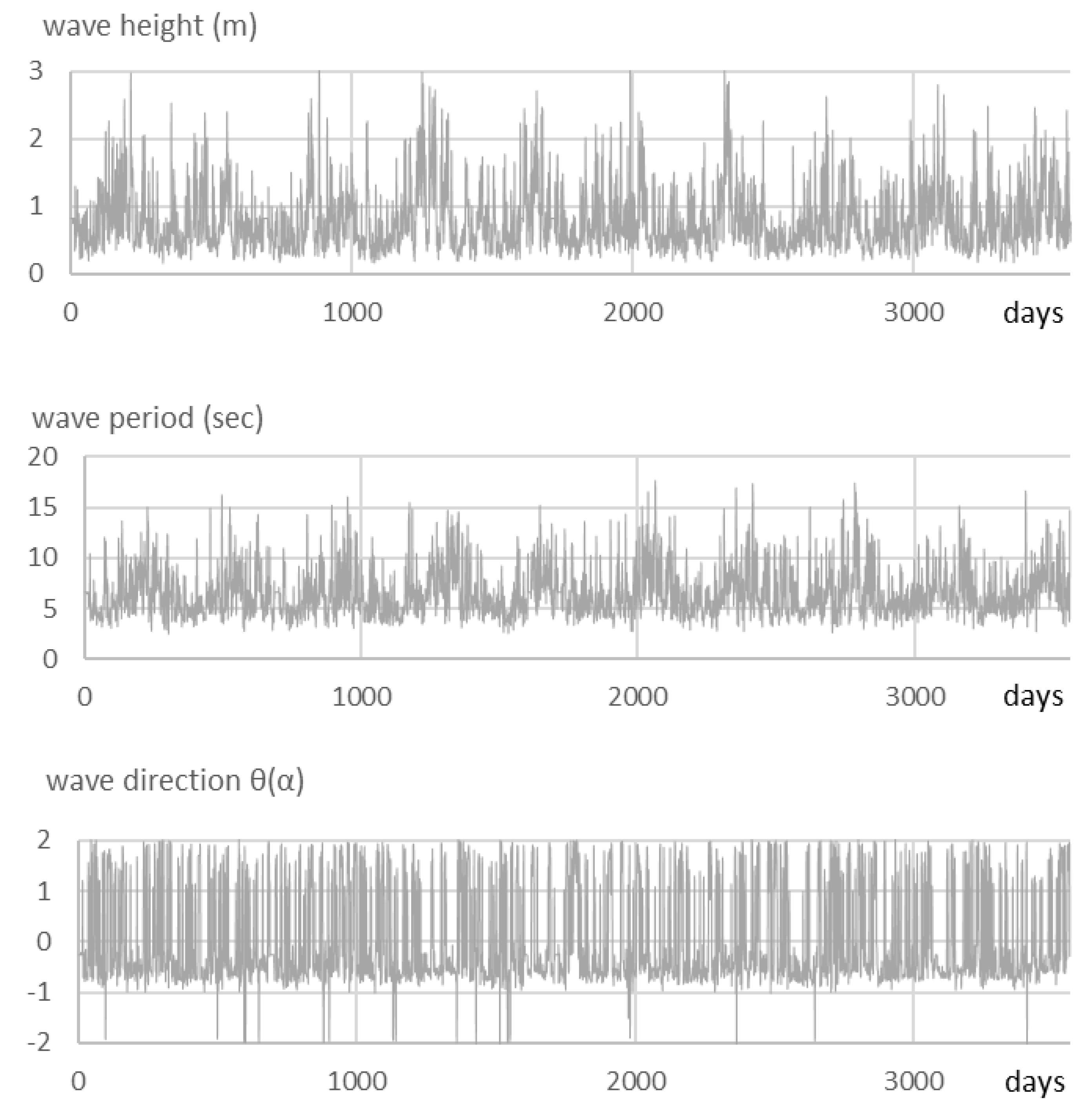
4. Simulation Results
5. Discussion and Conclusions
Supplementary Materials
Author Contributions
Funding
Institutional Review Board Statement
Informed Consent Statement
Data Availability Statement
Acknowledgments
Conflicts of Interest
Appendix A
Appendix B
- (1)
- Construct the covariance matrix P and find Q such that P = QQ′, wherewhere Γ′ is the transpose matrix of Γ.
- (2)
- Obtain the initial value (z−p+1,z−p+2,...,z0) by simulating vi ∼ N(0,1), where i = 1, ..., 3p, and letting (z−p+1,z−p+2,...,z0) = Q(v1,v2,...,v3p)>′.
- (3)
- Find matrix Q1 such that
- (4)
- Obtain simulated data for utby letting ut= Q1(v1t,v2t,v3t)′, where vkt ~ N(0,1), k = 1 ,2 , 3 and t = 1, 2,..., T, where T is the length of the simulated data.
- (5)
- Obtain the simulated data for the base process ztby letting
References
- Jägera, W.S.; Nagler, T.; Czado, C.; McCall, R.T. A statistical simulation method for joint time series of non-stationary hourly wave parameters. J. Coast. Eng. 2019, 146, 14–31. [Google Scholar] [CrossRef] [Green Version]
- Borgman, L.E.; Scheffner, N.W. Simulation of Time Sequences of Wave Height, Period, and Direction; Technical Report DRP-91-2, USACE-WDC; Coastal Engineering Research Center: Vicksburg, MS, USA, 1991. [Google Scholar]
- Callaghan, D.; Nielsen, P.; Short, A.; Ranasinghe, R. Statistical simulation of wave climate and extreme beach erosion. J. Coast. Eng. 2008, 55, 375–390. [Google Scholar] [CrossRef]
- Corbella, S.; Stretch, D.D. Predicting coastal erosion trends using non-stationary statistics and process-based models. J. Coast. Eng. 2012, 70, 40–49. [Google Scholar] [CrossRef]
- Li, J.; Winker, P. Time Series Simulation with Quasi Monte Carlo Methods. Comput. Econ. 2003, 21, 23–43. [Google Scholar] [CrossRef]
- Barone, P. A method for generating independent realizations of a multivariate normal stationary and invertible ARMA(p, q) process. J. Time Ser. Anal. 1987, 8, 125–130. [Google Scholar] [CrossRef]
- Shea, B.L. A Note on the generation of independent realizations of a vector autoregressive moving-average process. J. Time Ser. Anal. 1988, 9, 403–410. [Google Scholar] [CrossRef]
- Camus, P.; Mendez, F.J.; Medina, R.; Cofiño, A.S. Analysis of clustering and selection algorithms for the study of multivariate wave climate. J. Coast. Eng. 2011, 58, 453–462. [Google Scholar] [CrossRef]
- Soares, C.G.; Cunha, C. Bivariate autoregressive models for the time series of significant wave height and mean period. J. Coast. Eng. 2000, 40, 297–311. [Google Scholar] [CrossRef]
- Cai, Y. Multivariate time series simulation. J. Time Ser. Anal. 2011, 32, 566–579. [Google Scholar] [CrossRef]
- Cai, Y.; Gouldby, B.; Hawkes, P.; Dunning, P. Statistical Simulation of Flood Variables: Incorporating Short-Term Sequencing. J. Flood Risk Manag. 2008, 1, 1–10. [Google Scholar] [CrossRef]
- Cario, M.C.; Nelson, B.L. Numerical methods for fitting and simulating autoregressive-to-anything processes. J. Comput. 1998, 10, 72–81. [Google Scholar] [CrossRef] [Green Version]
- Biller, B.; Nelson, B.L. Modeling and generating multivariate timeseries input processes using a vector autoregressive technique. ACM Trans. Modeling Comput. Simul. (TOMACS) 2003, 13, 211–237. [Google Scholar] [CrossRef]
- Cai, Y.; Huang, J.; Tang, Y.; Zhou, G. A simulation method for finite non-stationary time series. J. Stat. Comput. Simul. 2014, 84, 1563–1579. [Google Scholar] [CrossRef] [Green Version]
- Ghaderpour, E.; Pagiatakis, S.D.; Hassan, Q.K. A Survey on Change Detection and Time Series Analysis with Applications. Appl. Sci. 2021, 11, 6141. [Google Scholar] [CrossRef]
- Looney, D.; Adjei, T.; Mandic, D.P. A Novel Multivariate Sample Entropy Algorithm for Modeling Time Series Synchronization. Entropy 2018, 20, 82. [Google Scholar] [CrossRef] [PubMed] [Green Version]
- Zhang, X.; Li, Y.; Gao, S.; Ren, P. Ocean Wave Height Series Prediction with Numerical Long Short-Term Memory. Mar. Sci. Eng. 2021, 9, 514. [Google Scholar] [CrossRef]
- Fuller, W.A. Introduction to Statistical Time Series, 1st ed.; John Wiley and Sons: New York, NY, USA, 1976. [Google Scholar]
- Mathworks. Available online: https://www.mathworks.com/help/econ/adftest.html#d123e114490 (accessed on 21 January 2022).
- Brockwell, P.J.; Davis, R.A. Time Series: Theory and Methods; Springer: New York, NY, USA, 1991. [Google Scholar]
- Bradbury, A.; Mason, T.; Poate, T. Implications of the spectral shape of wave conditions for engineering design and coastal hazard assessment–evidence from the English Channel. In Proceedings of the 10th International Workshop on Wave Hindcasting and Forecasting and Coastal Hazard Symposium, North Shore, Oahu, HI, USA, 11–16 November 2007. [Google Scholar]
- Silverman, B.W. Density Estimation for Statistics and Data Analysis. In Monographs on Statistics and Applied Probability; Chapman and Hall: London, UK, 1986. [Google Scholar]


Publisher’s Note: MDPI stays neutral with regard to jurisdictional claims in published maps and institutional affiliations. |
© 2022 by the authors. Licensee MDPI, Basel, Switzerland. This article is an open access article distributed under the terms and conditions of the Creative Commons Attribution (CC BY) license (https://creativecommons.org/licenses/by/4.0/).
Share and Cite
Valsamidis, A.; Cai, Y.; Reeve, D.E. Simulation of Wave Time Series with a Vector Autoregressive Method. Water 2022, 14, 363. https://doi.org/10.3390/w14030363
Valsamidis A, Cai Y, Reeve DE. Simulation of Wave Time Series with a Vector Autoregressive Method. Water. 2022; 14(3):363. https://doi.org/10.3390/w14030363
Chicago/Turabian StyleValsamidis, Antonios, Yuzhi Cai, and Dominic E. Reeve. 2022. "Simulation of Wave Time Series with a Vector Autoregressive Method" Water 14, no. 3: 363. https://doi.org/10.3390/w14030363
APA StyleValsamidis, A., Cai, Y., & Reeve, D. E. (2022). Simulation of Wave Time Series with a Vector Autoregressive Method. Water, 14(3), 363. https://doi.org/10.3390/w14030363