Scattering of Nonlinear Periodic (Cnoidal) Waves by a Partially Immersed Box-Type Breakwater

Abstract

This paper presents a combined analytical and numerical (CAN) model to simulate the scattering of cnoidal waves by a fixed and partially immersed box-type breakwater. A set of Boussinesq equations are solved in the outer region using the finite-difference method to model the propagation of cnoidal waves and their subsequent reflection and transmission after encountering the breakwater. The two-dimensional (2D) velocity potential in the inner region beneath the body is derived analytically by solving the equations formulated from the orthogonality of eigenfunctions and the interfacial matching conditions. Experimental measurements on the wave profiles were carried out in a wave tank to verify the model solutions. Reflected and transmitted wave elevations obtained from the present CAN model match closely with the measured data. Additionally, the calculated horizontal and vertical forces on the body using the developed CAN model are in reasonable agreement with those from a potential 2D flow-based fully nonlinear wave model (FNWM). The method and proposed CAN model, if applied to a simple parametric investigation, can provide the expected trends in terms of applied forces, wave reflection, and transmission.

1. Introduction

Over the past few decades, the action of water waves on nearshore structures has been one of the most interesting and important topics investigated by researchers and engineers to obtain the wave elevations and applied forces needed for coastal protection-related projects. A partially immersed breakwater, in general, can be placed as an economic and effective protective structure to reduce the direct action of an incoming wave and at the same time to maintain the needed environmental conditions for water behind the body through the induced fluid motion across the region beneath the body.

Early studies on waves acting on a partially immersed or fixed floating body focused mostly on the use of a linear wave as an incident wave condition. Mei and Black [1] introduced a variational-formulation-based numerical approach to calculate the scattering properties of a linear wave for bottom and surface obstacles of various proportions, including surface docks. Later, the scattering of a regular wave by a fixed and partially immersed circular cylinder was investigated by Martin and Dixon [2]. Also limited to the linear wave condition, McCartney [3] examined the advantages and disadvantages of the box and pontoon type of breakwaters using the hydraulic model test results. Based on the assumption of a small gap condition, Drimer et al. [4] derived a simplified analytical model to study the effectiveness of a partially submerged long rectangular breakwater in reducing the transmitted waves. Solving the symmetric and antisymmetric parts of the velocity potentials analytically, Kanoria et al. [5] analyzed the behavior of the reflection coefficient for a linear wave encountering four types of fixed obstacles in the form of a thick rectangular cross-section that was placed in different vertical positions, including a partially immersed one. Considering two porous walls attached to a partially submerged box type breakwater, Qiao et al. [6] analytically and experimentally investigated the performance of the breakwater in reducing the reflected and transmitted linear waves under various structural and porous wall conditions. Recently, an analytical approach was carried out by Kaligatla [7] to study the oblique scattering of a linear water wave by a partially immersed rectangular breakwater.

The above-mentioned studies on linear waves acting on a fixed and partially immersed body may not represent well the wave conditions in coastal areas of shallow water depth, especially when the wave height becomes relatively large. Therefore, it is desirable to extend the linear wave study to cases with the inclusion of wave nonlinearity in shallow-water depth by modeling the wave propagation, wave transformation, and induced wave forces on bodies. Solitary and cnoidal waves are two typical nonlinear water waves that propagate in a domain of shallow-water depth, or the so-called Boussinesq-type waves. Because of its simple bell-shaped-like wave form, the wave scattering between a solitary wave and various structures of interest were investigated more often than those using a cnoidal wave with periodic oscillations as an incident wave condition. Adopting a linearized wave diffraction theory and a Fourier transformation technique, Isaacson [8] derived an approximated analytical solution to calculate the applied wave forces for a solitary wave encountering a bottom-mounted and surface-piercing circular cylinder. For a similar structural condition, Wang et al. [9] and Zhong and Wang [10] numerically solved the full nonlinear Boussinesq equations to model the scattering process of a solitary wave acting on a fixed vertical cylinder or a cylinder group. In terms of the cases for a solitary wave propagating past a partially submerged body, the wave reflection and transmission processes were investigated by Lu and Wang [11], Xu et al. [12]; and Chang et al., [13] for a box-type structure and by Chen and Wang [14] for a circular cylinder.

A cnoidal wave with its periodic oscillatory feature is probably better represented when considering waves propagating in a shallow-water coastal environment. Therefore, as modeling studies on cnoidal waves have been very limited, there is a need to expand the approaches to solve the problems related to cnoidal waves encountering a coastal structure. The studies of scattering of cnoidal waves by either a single or multiple bottom-mounted and surface-piercing cylinders include the early theoretical or modeling efforts carried out by Isaacson [15] and Wang and Ren [16], and more recently by Weng et al. [17] and Zhang and Teng [18]. Tang and Lee [19] investigated the generation of cnoidal waves and their induced oscillatory boundary-layer flow over a wavy bottom. Ren and Ma [20] numerically simulated the scattered wave patterns for cnoidal waves encountering a structured system of multiple perforated quasi-ellipse caissons by solving the Navier-Stokes equations with the finite-difference method and the volume-of-fluid technique to capture the free-surface elevations.

Overall, the problems related to a nonlinear shallow water wave acting on a bottom-mounted and surface-piercing obstacle have been investigated more often than in cases with a truncated (or partially immersed) structure. The no-flow boundary condition for a body extended from bottom to above the fluid surface can be applied uniformly to the entire structural boundary that is in contact with the fluids. However, for a partially immersed body, a special solution procedure needs to be developed to handle the mixed boundary conditions that are applied separately on the structural surface and the interfacial open boundaries connecting the inner and outer regions. Additionally, because of the periodic feature, based on modeling efforts, it is generally harder to use a cnoidal wave than a solitary wave to enter such an incident wave into the computational domain and to propagate the scattered and main waves out of the upstream and downstream open boundaries. The other numerical challenge that requires special attention is to model the standing waves or the resonant phenomenon when generated from a periodic flow passing through a confined lateral fluid domain either for a potential flow or a viscous flow condition [21,22,23]. In this study, the wave scattering process after a cnoidal wave has been propagated through the underneath open region does not include the phenomena of standing wave and wave resonance. Due to the lack of studies on a partially immersed body under a cnoidal wave condition, it is important to provide a new modeling approach to predict the wave variations and applied forces for a cnoidal wave encountering a structure that is partially submerged in water. In this study, we intend to develop an efficient and reliable model with a combined analytical and numerical (CAN) approach to investigate the propagation of a cnoidal wave and its subsequent scattering process after encountering a fixed but partially immersed 2D body of rectangular prism. For model verification, experimental measurements were also carried out to record the wave elevations at two locations upstream and downstream of the body. With both sidewalls of a rectangular structure extended vertically upward to a level, which is much higher than the encountering wave elevation, the effect of wave overtopping is not considered in the present study.

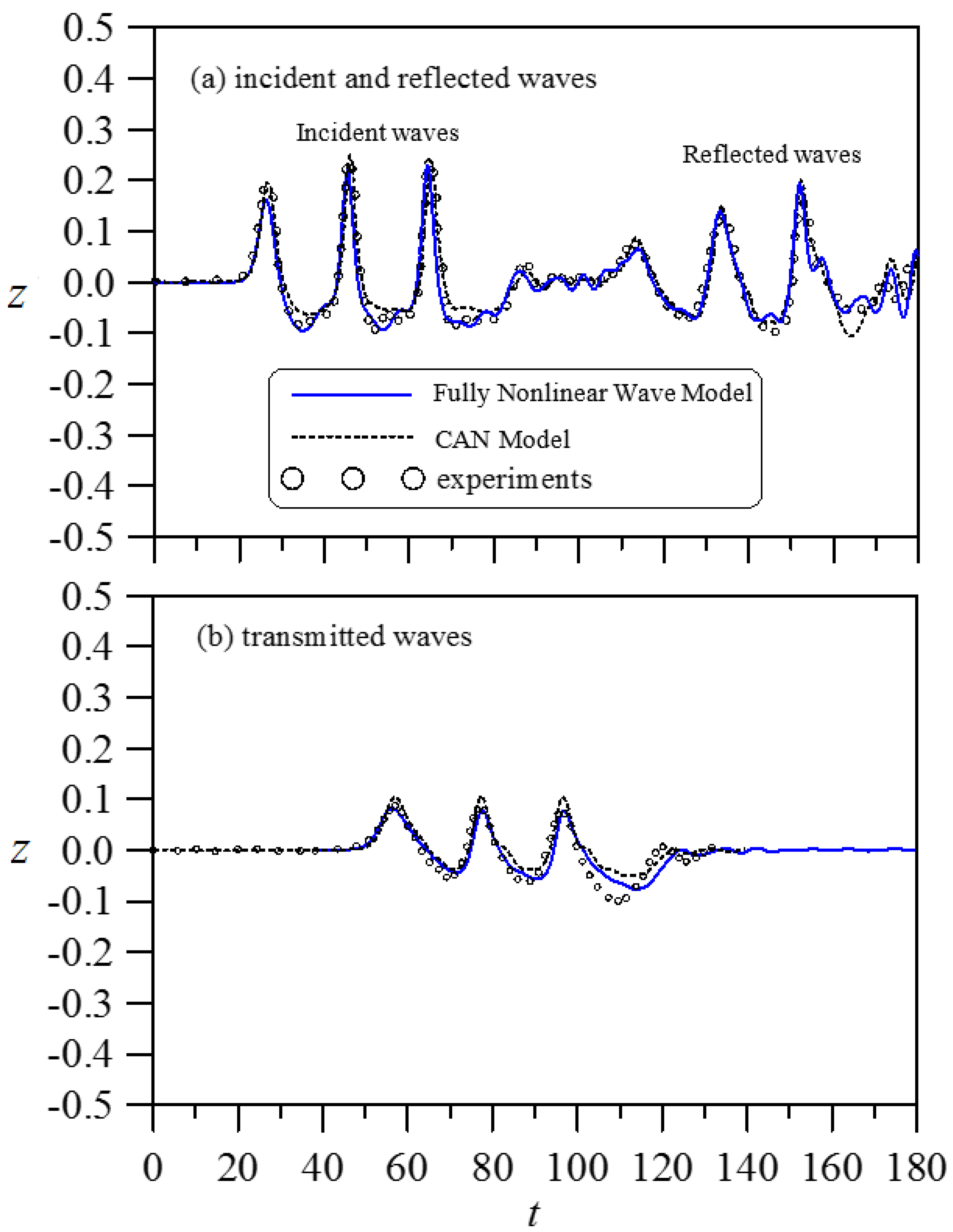
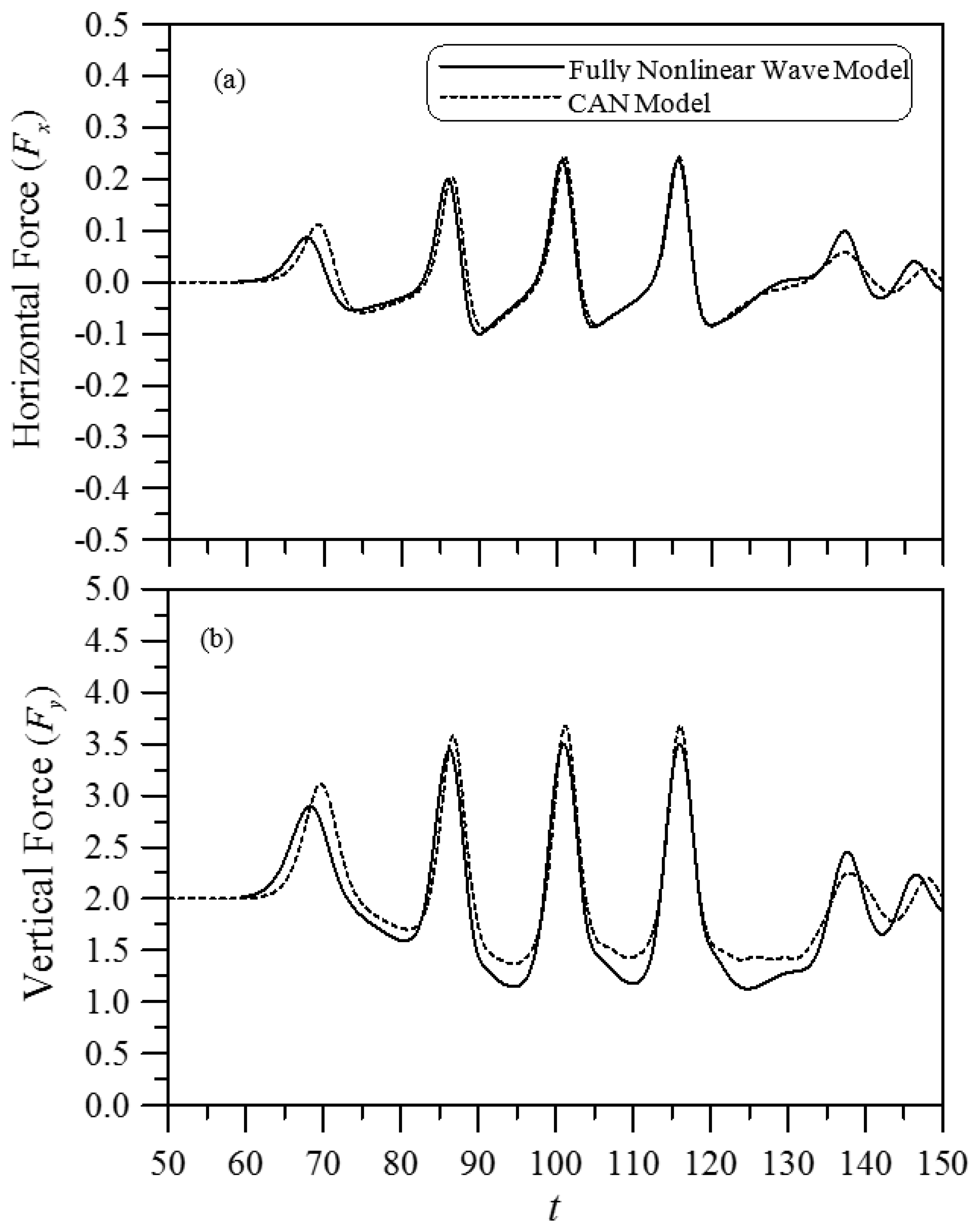
As a part of the integrated approach, a set of Boussinesq equations are solved in the outer region using the finite-difference method to obtain the wave field outside of the body. The solutions for fluid flows in the region beneath the partially immersed body are determined analytically by solving the equations formulated from the orthogonality of eigenfunctions and the mixed matching conditions formed at the domain interfaces. In addition to the determination of the free-surface elevations in terms of the reflected and transmitted waves, the hydrodynamic forces on the solid surface of the truncated structure are calculated. The measurements of incident, reflected, and transmitted wave profiles under different waves and structural conditions are used to verify the model predictions. The CAN model results match closely with the measured data. The CAN model calculated horizontal and vertical forces on the body that were then compared with the results obtained from a potential-flow-based fully nonlinear wave model (FNWM). The agreeable force comparisons from the two models are considered to effectively verify the feasibility and applicability of the CAN model. The parametric studies by examining the effects of body thickness and immersed depth (draft) on the reflected and transmitted waves are also presented.

The fully nonlinear wave model (FNWM)—adopted to make comparisons with the CAN model results—was developed by Chang et al. [13]. This numerical model solved the Laplace equation of the velocity potential describing the vertical 2D flow field together with the fully nonlinear kinematic and dynamic free-surface boundary conditions in a transient boundary-fitted grid system. The grids generated follow the transient curvilinear coordinate system, which transforms the time-dependent physical domain in (x, y; t) to a computational domain in ($\xi$, $\eta$; $\tau$). The spatial discretization of the governing differential equation in the model was based on the up to second-order accuracy finite difference scheme and the time derivative is approximated with a forward difference. More detailed theoretical and numerical formulations, computational procedures, and verification of the FNWM can be found in Chang et al. [13].

The aim of the present study is to advance the knowledge on the development of a combined analytical and numerical (CAN) approach to improve the computational efficiency and stability for predicting the scattering process of an incident nonlinear shallow-water wave, such as the cnoidal wave, encountering a partially immersed box-type body. The main advantage of the CAN model when compared to the fully nonlinear wave model (FNWM) is its computational efficiency. Even for a vertical two-dimensional (2D) domain, the FNWM requires a layout of a large number of 2D grid points for intensive calculations, which is considered computationally expensive. However, the CAN model can perform calculations under a one-dimensional grid system for the fluid regions outside of a partially immersed box-type body. The solutions are determined analytically for the region beneath the body. The CAN model is more efficient in producing the results. Additionally, the FNWM will encounter the typical instability issue when solving the equations at the corner points of the fluid domain unless special numerical treatments or approximations are applied at those grid points. Those approximated numerical procedures may affect the accuracy of the calculations at the interfacial regions. As for the CAN model, the solutions for the fluid region beneath the body (including the corner points) are analytically determined; the calculation of the vertical force can be more accurately and effectively evaluated. Considering the prediction of the wave profiles, the CAN model can calculate the free-surface elevations directly by solving the Boussinesq equations and does not need the implementation of special numerical techniques to capture the movement of the free surface as the FNMW does.

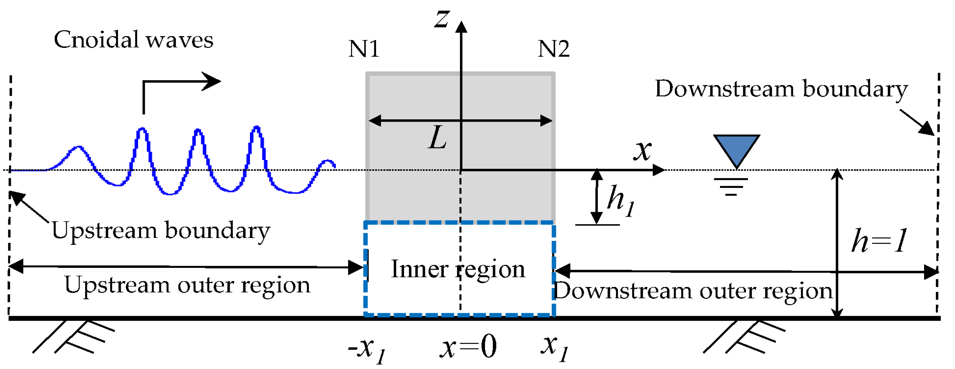
The CAN approach applied in this study integrates the procedure of numerical simulations of the propagation and diffraction process of the cnoidal waves in the region outside of a fixed and partially immersed rectangular body (outer region) and analytical calculations of the flow solutions in the region beneath the body (inner region). Presented in the following two sections are the basic model equations, boundary conditions, initial conditions, and derived solutions with calculation procedures for the domains of the outer and inner regions.

2. Mathematical Formulations

A sketch of the 2D problem statement showing a sequence of cnoidal waves propagating towards a partially immersed rectangular body is shown in Figure 1. As mentioned above, the fluid domain under the partially immersed body is the inner region (or region 2) while the domain including the upstream and downstream regions of the body is the outer region (region 1). For the convenience of expressing the governing equations and boundary conditions in a dimensionless form, all physical variables without the “*” symbol are nondimensionalized using the undisturbed water depth ($h_0^{*}$), celerity of the linear long wave ($c_0^{*}=\sqrt{g{h}_0^{*}}$), and $h_0^{*}/c_0^{*}$ as the length, velocity, and time scales, respectively, where g is the gravitational acceleration. The dimensionless water depth in region 1 is defined as h = 1 (flat bottom condition) and the draft (submergence of the body) is set as $h_1$. For the potential flow condition, the fluid is assumed to be incompressible and the motion irrotational. The effect of fluid viscosity is neglected. The 2D Cartesian coordinate system (x, z) defines the spatial domain. The bottom boundary of the fluid domain is set at z = −1 while z = $\mathsf{\zeta }$ (x, t) is used to prescribe the free surface of the wave motion referenced to the undisturbed free surface at z = 0.

2.1. Model Equations and Boundary Conditions for Fluids in the Outer Region

A cnoidal wave—as a weakly nonlinear and weakly dispersive wave—belongs to the class of Boussinesq wave systems. Accordingly, the Boussinesq equations for a constant water depth are adopted as the governing equations to model the propagation, reflection, and transmission of the cnoidal waves in the outer region. The dimensionless form of the Boussinesq equations is expressed as:

$${\mathsf{\zeta }}_t+\nabla \cdot [\left(1+\mathsf{\zeta }\right)\nabla \overline{\varphi }]=0,$$

(1)

$${\overline{\varphi }}_t+\frac{1}{2}{(\nabla \overline{\varphi })}^2-\frac{1}{3}{\nabla }^2{\overline{\varphi }}_t+\mathsf{\zeta }=0,$$

(2)

where $\overline{\varphi }(x,t)$ is the depth-averaged dimensionless velocity potential. When related to the original velocity potential $\varphi (x,z,t)$, we have $\overline{\varphi } (x,t)=[{\displaystyle {\int }_{-1}^{\mathsf{\zeta }}\varphi (x,z,t)dz}]/(1+\mathsf{\zeta })$. The subscript t denotes the time derivative, $\nabla =(\partial /\partial x,\partial /\partial z)$ is the two-dimensional gradient operator and ${\nabla }^2=({\partial }^2/\partial x^2+{\partial }^2/\partial z^2)$ is the Laplacian operator. By using the standard expansion method, the relationship between $\varphi (x,z,t)$ and $\overline{\varphi }(x,t)$ can be derived by neglecting the higher order terms as

$$\varphi =\overline{\varphi }+\frac{{\mu }^2}{6}{(\mathsf{\zeta }+1)}^2{\nabla }^2\overline{\varphi }-\frac{{\mu }^2}{2}{(z+1)}^2{\nabla }^2\overline{\varphi },$$

(3)

where ${\mu }^2={(h_0^{*}/{\lambda }^{*})}^2$ is a dimensionless parameter measuring the wave dispersive effect and ${\lambda }^{*}$ is the dimensional wave length.

Appropriate boundary conditions are required to be implemented when solving Equations (1) and (2) numerically in the outer region. At the submerged left and right faces of the body, the no-flow condition is applied, i.e.,

$$\frac{\partial \varphi }{\partial x}=0 -h_1\le z\le \mathsf{\zeta } \mathrm{at} x=x_1 \mathrm{and} x=-x_1.$$

(4)

Additionally, the open boundary conditions are solved to allow the incident waves to move into the computational domain and propagate the waves out of the downstream boundary without adversely influencing the waves in the domain of interest. In this study, a set of simple wave equations (the so-called Sommerfeld radiation conditions) with specified phase speeds, similar to those applied successfully to model the propagation of cnoidal waves and their scattered wave patterns after encountering cylinders [16,21,24], are used as the open boundary conditions. At the upstream boundary, we have:

$$\frac{\partial \overline{\varphi }}{\partial t}-c_0\frac{\partial \overline{\varphi }}{\partial x}=\frac{\partial {\overline{\varphi }}^I}{\partial t}-c_0\frac{\partial {\overline{\varphi }}^I}{\partial x},$$

(5a)

$$\frac{\partial \mathsf{\zeta }}{\partial t}-c_0\frac{\partial \mathsf{\zeta }}{\partial x}=\frac{\partial {\mathsf{\zeta }}^I}{\partial t}-c_0\frac{\partial {\mathsf{\zeta }}^I}{\partial x}.$$

(5b)

At the downstream boundary, the following conditions are applied,

$$\frac{\partial \overline{\varphi }}{\partial t}+c\frac{\partial \overline{\varphi }}{\partial x}=0,$$

(6a)

$$\frac{\partial \mathsf{\zeta }}{\partial t}+c\frac{\partial \mathsf{\zeta }}{\partial x}=0,$$

(6b)

where ${\overline{\varphi }}^I$ and ${\mathsf{\zeta }}^I$ represent, respectively, the depth-averaged velocity potential and free-surface elevation of the incident cnoidal wave. Their formulations are summarized in Section 2.3. The c is the dimensionless phase velocity of the incident wave and $c_0=1$.

2.2. Model Equations and Boundary Conditions for Fluids in the Inner Region

For the inner region (region 2) beneath a partially immersed body, its velocity potential ${\phi }_2(x,z,t)$ under the assumed potential flow condition satisfies the usual Laplace equation:

$${\nabla }^2{\phi }_2=0 -1\le z\le -h_1, \mathrm{and}-x_1\le x\le x_1.$$

(7)

The boundary conditions of zero normal velocity are applied at the flat domain bottom and the solid bottom surface of the body, which give:

$$\frac{\partial {\phi }_2}{\partial z}=0 at z=-h_1 \mathrm{and} z=-1.$$

(8)

To connect continuously the outer and inner solutions, the specified matching conditions for the velocities and velocity potentials at the interfaces $x=-x_1$ and $x=x_1$ (Figure 1) are:

$$\frac{\partial \varphi }{\partial x}=\frac{\partial {\phi }_2}{\partial x} -1\le z\le -h_1 \mathrm{at} x=x_1 \mathrm{and} x=-x_1,$$

(9)

$$\varphi ={\phi }_2 -1\le z\le -h_1 \mathrm{at} x=x_1 \mathrm{and} x=-x_1.$$

(10)

2.3. Incident Cnoidal Waves

To model the propagation and subsequent scattering process after the cnoidal waves encounter a partially immersed 2D body, the inputs of a group of incident cnoidal waves from the left open boundary are required. Similar to the cnoidal wave solutions given in Sarpkaya and Isaacson [25], in this study, a set of modified dimensionless forms of the second-order cnoidal wave solutions of the Boussinesq equations (Equations (1) and (2)) from Jiang and Wang [24] are adopted as the incident wave conditions. For a plane right-going cnoidal wave, we have:

$${\mathsf{\zeta }}^I=\alpha [c{n}^2(q,m)-f_1]-{\alpha }^2\left\{\frac{3}{4}c{n}^2(q,m)[1-c{n}^2(q,m)]+f_2\right\},$$

(11)

$$c=1+\alpha c_1+{\alpha }^2{c}_2,$$

(12)

$${\overline{u}}^I=\alpha [c{n}^2(q,m)-f_1]+{\alpha }^2\left[r_1+r_2 c{n}^2(q,m)-\frac{c{n}^4(q,m)}{4}\right].$$

(13)

The expressions $m_1$, $q$, $\gamma$, $c_1$, $c_2$, $f_1$, $f_2$, $r_1$, and $r_2$ appearing in Equations (11)–(13) are summarized in Appendix A. Other notations are defined as: $\alpha =H^{*}/h_0^{*}$ = dimensionless wave height; $H^{*}$ = dimensional wave height; ${\mathsf{\zeta }}^I$ = wave elevation of an incident cnoidal wave; ${\overline{u}}^I$ = depth-averaged velocity of an incident cnoidal wave; $cn(q,m)$ = Jacobian elliptic function with argument q and modulus m; $K(m)$ = complete elliptic integral of the first kind; $E(m)$ = complete elliptic integral of the second kind; $k=2\pi /{\lambda }^{*}$ = wave number; $\omega =2\pi /T^{*}$ = wave frequency; and $T^{*}$ = dimensional wave period. The dimensionless wave length is defined as $\lambda ={\lambda }^{*}/h_0^{*}$. Up to the leading order of α, it can be seen in Equations (11) and (13) that the expressions of dimensionless wave elevation ${\mathsf{\zeta }}^I$ and depth-averaged velocity ${\overline{u}}^I$ are the same. This is a typical long wave condition. Additionally, the oscillation of either the wave elevation or the depth-averaged velocity is dominated by the function of $c{n}^2(q,m)$.

By integrating the velocity formulation given in Equation (13), the depth-averaged velocity potential ${\overline{\varphi }}^I$ for an incident cnoidal wave can be evaluated conveniently using the following expression series [24].

$${\overline{\varphi }}^I=\frac{-i\alpha }{k{h}_0^{*}}\left\{{\displaystyle \sum _{n=1}^{\infty }\left[\frac{A_n+\alpha B_n}{n}\right]e^{ink{h}_0^{*}(x-ct)}}\right\}+{\alpha }^2\left[\frac{\gamma (-3\gamma -2m+4)-m_1}{6m^2}\right](x-ct).$$

(14)

where “i” is the imaginary unit. In Equation (14), the coefficients $A_n$ and $B_n$ are calculated according to the formulations given, respectively, as:

$$A_n=\frac{4{\pi }^2}{m{K}^2(m)}{C}_n,$$

(15a)

$$B_n=\frac{m-2}{4m}{A}_n-\frac{1}{8}{\displaystyle \sum _{j=1}^{n-1}{A}_j{A}_{n-j}}-\frac{1}{4}{\displaystyle \sum _{j=1}^{\infty }{A}_j{A}_{n+j}},$$

(15b)

where

$$C_n=\frac{1}{2}{\displaystyle \sum _{j=1}^{2n-1}{\beta }_j{\beta }_{2n-j}}+{\displaystyle \sum _{j=1}^{\infty }{\beta }_j{\beta }_{2n+j}} \left\{\begin{array}{l}{\beta }_j=0 \mathrm{when} j \mathrm{is} \mathrm{even},\\ {\beta }_j={\vartheta }^{j/2}/(1+{\vartheta }^j) \mathrm{when} j \mathrm{is} \mathrm{odd}.\end{array}\right\}.$$

(15c)

Here, $\vartheta =\exp \left[-\pi K(m_1)/K(m)\right]$. The formulas of wave elevation and depth-averaged velocity potential (Equations (11) and (14)) are applied as the incident wave condition for modeling the propagation of cnoidal waves in the outer region.

3. A Coupled Solution Procedure by Combining the Analytical and Numerical Solutions

3.1. Numerical Solutions in the Outer Region

In this study, a coupled solution procedure by combining the inner analytical solutions and the outer numerical solutions is used to model the encountering process between cnoidal waves and a partially immersed rectangular body. Numerically, the spatial grid indices describing the variables at the outer region are assigned as i = 1, 2, 3, …, N1 − 1 in front of the left interface and i = N2 + 1,…, Nmax behind the right interface. The outer solutions are determined by solving the Boussinesq equations (Equations (1) and (2)) in the domain of i = 2, 3, …, N1 − 1 and i = N2 + 1,…, (Nmax − 1) based on the modified Euler’s predictor-corrector finite-difference scheme [9]. Separately, the boundary conditions (Equations (5) and (6)) are applied at i = 1 and Nmax of the left and right open boundaries, respectively. The spatial grid indices at the left interface ($x=-x_1$) and the right interface ($x=x_1$) are assigned as N1 and N2, respectively (see Figure 1). At a time level of $n\Delta t$, the depth-averaged velocity potential $\overline{\varphi }$ and wave elevation $\mathsf{\zeta }$ are expressed as ${\overline{\varphi }}_i^n=\overline{\varphi }(i\Delta x,n\Delta t)$ and ${\mathsf{\zeta }}_i^n=\mathsf{\zeta }(i\Delta x,n\Delta t)$, respectively. Here, $\Delta x$ is the grid size and $\Delta t$ denotes the time step.

The predictor-corrector finite-difference scheme, which is up to the second-order accuracy, was applied to solve the governing Equations (1) and (2). This numerical approach has been demonstrated in several prior studies [9,16,21,24] to produce stable and accurate solutions, especially for cases using either solitary or cnoidal waves as incident wave conditions. Solving the implicit finite-difference formulations at the corrector stage by means of the successive over-relaxation (SOR) iterative procedure with the inputs of the predictor values, the final solutions can be accurately determined and no numerical noise was observed. Summarized in Appendix B are the detailed numerical formulations for the determination of ${\overline{\varphi }}_i^{n+1}$ and ${\mathsf{\zeta }}_i^{n+1}$ at the new time level of $(n+1)\Delta t$. It is noted that the needed values of ${\overline{\varphi }}_{N1}$ and ${\overline{\varphi }}_{N2}$ at the interfaces are evaluated from the coupled inner solutions and matching conditions, which are described in the section of the inner solutions given below.

It should be noted that the wave elevation (Equation (11)) and depth-averaged velocity potential (Equation (14)) from the cnoidal wave theory are only used as the incident wave conditions at the upstream open boundary through the application of the open boundary conditions (Equations (5a) and (5b)). The depth-averaged velocity potentials and free-surface elevations for the outer region (excluding the upstream and downstream open boundaries) are computed by solving numerically the Boussinesq equations as described above and in Appendix B.

3.2. Analytical Solutions in the Inner Region

The coupled formulations derived for the determination of the inner velocity potential, the associated solution coefficients, and the interfacial values of ${\overline{\varphi }}_{N1}$ and ${\overline{\varphi }}_{N2}$ are introduced in this subsection. To describe the fluid motions as waves passing through the region beneath a partially immersed body (inner region), the analytical solution of the velocity potential ${\phi }_2$ is derived as:

$${\phi }_2={\displaystyle \sum _{j=1}^{\infty }\left(A_j\cosh \left(k_{j}x\right)+B_j\sinh \left(k_{j}x\right)\right)}\cos k_j\left(z+1\right)+Cx+D,$$

(16)

where $A_j$, $B_j$ $(j=1,2,\dots )$, C, and D are solution coefficients and $k_j$ $(j=1,2,\dots )$ are the eigenvalues, which are defined as $k_j=j\pi /(1-h_1)$. Based on the matching condition in Equation (10) and the orthogonal properties of the eigenfunctions, $\cos k_j(z+1)$, over the interval of $-1\le z\le -h_1$, we have:

$${\displaystyle \underset{-1}{\overset{-h_1}{\int }}{\phi }_2}(x,z)\cos (k_j(z+1))dz={\displaystyle \underset{-1}{\overset{-h_1}{\int }}{\varphi }_{N1}(x,z)\cos (k_j(z+1))}dz \mathrm{at} x=-x_1,$$

(17)

In addition,

$${\displaystyle \underset{-1}{\overset{-h_1}{\int }}{\phi }_2}(x,z)\cos (k_j(z+1))dz={\displaystyle \underset{-1}{\overset{-h_1}{\int }}{\varphi }_{N2}(x,z)\cos (k_j(z+1))}dz \mathrm{at} x=x_1,$$

(18)

Here, ${\varphi }_{N1}$ and ${\varphi }_{N2}$ represent the original 2D velocity potentials at the left and right interfaces, respectively. Additionally, by extending the matching conditions (Equation (10)) at $x=-x_1 \mathrm{and} x=x_1$ from $z=-1$ to $z=-h_1$, we have:

$${\displaystyle \underset{-1}{\overset{-h_1}{\int }}{\varphi }_{N1}}dz={\displaystyle \underset{-1}{\overset{-h_1}{\int }}{\phi }_2}dz \mathrm{at} x=-x_1,$$

(19)

$${\displaystyle \underset{-1}{\overset{-h_1}{\int }}{\varphi }_{N2}}dz={\displaystyle \underset{-1}{\overset{-h_1}{\int }}{\phi }_2}dz \mathrm{at} x=x_1,$$

(20)

Substituting Equations (3) and (16) into Equations (17) and (18) and utilizing Equations (19) and (20) for a given j (j = 1, 2,…), Equations (17) and (18) can be converted into:

$$A_j\cosh (k_j{x}_1)-B_j\sinh (k_j{x}_1)=-\frac{2{\mu }^2(1-h_1)}{k_j{}^2\Delta x^2{P}_{11}}\cos (k_j(1-h_1))[(-x_1)C+D-{\overline{\varphi }}_{N1}],$$

(21)

$$A_j\cosh (k_j{x}_1)+B_j\sinh (k_j{x}_1)=-\frac{2{\mu }^2(1-h_1)}{k_j{}^2\Delta x^2{P}_{21}}\cos (k_j(1-h_1))[x_{1}C+D-{\overline{\varphi }}_{N2}],$$

(22)

where $\Delta x$ is the grid size and,

$$P_{11}=\frac{{\mu }^2}{6\Delta x^2}[{(1+{\mathsf{\zeta }}_{N1})}^2(1-h_1)-{(1-h_1)}^3],$$

(23)

$$P_{21}=\frac{{\mu }^2}{6\Delta x^2}[{(1+{\mathsf{\zeta }}_{N2})}^2(1-h_1)-{(1-h_1)}^3].$$

(24)

Here, ${\mathsf{\zeta }}_{N1}$ and ${\mathsf{\zeta }}_{N2}$ are wave elevations at the left ($x=-x_1$) and right ($x=x_1$) interfaces, respectively. Then, the unknown coefficients, $A_j$ and $B_j$ $(j=1,2,\dots M)$ can be calculated by solving Equations (21) and (22) simultaneously, where M is the total number of terms in Equation (16) to have a converged solution. The determination of two other coefficients, C and D, and variables, ${\overline{\varphi }}_{N1}$ and ${\overline{\varphi }}_{N2}$, are described in the following.

The application of the depth-averaged outer-region velocity potentials at point N1 (at $x=-x_1$) and N2 (at $x=x_1$) leads to:

$${\overline{\varphi }}_{N1} =\frac{1}{1+{\mathsf{\zeta }}_{N1}}{\displaystyle \underset{-1}{\overset{{\mathsf{\zeta }}_{N1}}{\int }}{\varphi }_{N1}(x,z,t)dz}=\frac{1}{1+{\mathsf{\zeta }}_{N1}}\left[{\displaystyle \underset{-1}{\overset{-{\mathrm{h}}_1}{\int }}{\phi }_2(x,z,t)dz+{\displaystyle \underset{-{\mathrm{h}}_1}{\overset{{\mathsf{\zeta }}_{N1}}{\int }}{\varphi }_{N1}(x,z,t)dz}}\right],$$

(25)

$${\overline{\varphi }}_{N2} =\frac{1}{1+{\mathsf{\zeta }}_{N2}}{\displaystyle \underset{-1}{\overset{{\mathsf{\zeta }}_{N2}}{\int }}{\varphi }_{N2}(x,z,t)dz}=\frac{1}{1+{\mathsf{\zeta }}_{N2}}\left[{\displaystyle \underset{-1}{\overset{-{\mathrm{h}}_1}{\int }}{\phi }_2(x,z,t)dz+{\displaystyle \underset{-{\mathrm{h}}_1}{\overset{{\mathsf{\zeta }}_{N2}}{\int }}{\varphi }_{N2}(x,z,t)dz}}\right].$$

(26)

By substituting Equations (3) and (16) of the outer and inner velocity potentials into the right-hand sides of Equations (25) and (26), two control equations can be derived:

$$(1+{\mathsf{\zeta }}_{N1}-P_{12}){\overline{\varphi }}_{N1}^{}=-x_1(1-h_1)C+(1-h_1)D+({\mathsf{\zeta }}_{N1}+h_1-2P_{12}){\overline{\varphi }}_{N1-1}^{}+P_{12}{\overline{\varphi }}_{N1-2}^{},$$

(27)

$$(1+{\mathsf{\zeta }}_{N2}-P_{22}){\overline{\varphi }}_{N2}^{}=x_1(1-h_1)C+(1-h_1)D+({\mathsf{\zeta }}_{N2}+h_1-2P_{22}){\overline{\varphi }}_{N2+1}^{}+P_{22}{\overline{\varphi }}_{N2+2}^{},$$

(28)

where

$$P_{12}=\frac{{\mu }^2}{6\Delta x^2}[{(1+{\mathsf{\zeta }}_{N1})}^2({\mathsf{\zeta }}_{N1}+h_1)-{(1+{\mathsf{\zeta }}_{N1})}^3+{(1-h_1)}^3]$$

(29)

$$P_{22}=\frac{{\mu }^2}{6\Delta x^2}[{(1+{\mathsf{\zeta }}_{N2})}^2({\mathsf{\zeta }}_{N2}+h_1)-{(1+{\mathsf{\zeta }}_{N2})}^3+{(1-h_1)}^3]$$

(30)

It is noted the derivations of Equations (27) and (28) utilize the finite-difference approximations of ${\nabla }^2{\overline{\varphi }}_{N1-1}=({\overline{\varphi }}_{N1}-2{\overline{\varphi }}_{N1-1}+{\overline{\varphi }}_{N1-2})/(\Delta x^2)$, ${\nabla }^2{\overline{\varphi }}_{N2+1}=({\overline{\varphi }}_{N2+2}-2{\overline{\varphi }}_{N2+1}+{\overline{\varphi }}_{N2})/(\Delta x^2)$, and the boundary condition given in Equation (4). Following the similar procedure given above; however, by using the matching condition of Equation (9) with the integration range from z = −1 to $z=-h_1$, two more control equations are derived:

$$P_{11}{\overline{\varphi }}_{N1}^{}=-(x_1+\Delta x)(1-h_1)C+(1-h_1)D+[2P_{11}-(1-h_1)]{\overline{\varphi }}_{N1-1}^{}-P_{11}{\overline{\varphi }}_{N1-2}^{}$$

(31)

$$P_{21}{\overline{\varphi }}_{N2}^{}=(x_1+\Delta x)(1-h_1)C+(1-h_1)D+[2P_{21}-(1-h_1)]{\overline{\varphi }}_{N2+1}^{}-P_{21}{\overline{\varphi }}_{N2+2}^{}$$

(32)

By solving Equations (27), (28), (31), and (32), the unknown coefficients, C and D, for the velocity potential of the inner region (${\phi }_2$) can be determined. Simultaneously, the unknown variables ${\overline{\varphi }}_{N1}$ and ${\overline{\varphi }}_{N2}$, which are needed for the numerical computations in the outer region and solving Equations (21) and (22), can also be calculated. It is noted that the required ${\overline{\varphi }}_{N1-1}^{},$ ${\overline{\varphi }}_{N1-2}^{}$, ${\overline{\varphi }}_{N2+1}^{}$, and ${\overline{\varphi }}_{N2+2}^{}$ values are numerically computed following the outer solution procedure given in Section 3.1.

4. Force Calculations

In addition to the prediction of wave transformation using the CAN model as described above, the induced hydrodynamic forces on the body are important variables to be determined. With the model calculated free-surface elevations and velocity components, the dimensionless horizontal force per unit width, $F_x=F_x{}^{*}/\rho g{(h_0^{*})}^2$, and vertical force per unit width, $F_z=F_z{}^{*}/\rho g{(h_0^{*})}^2$, can be computed by integrating the pressure along their corresponding structural surfaces, where $F_x{}^{*}$ and $F_z{}^{*}$ are, respectively, the dimensional horizontal and vertical forces per unit width. We have:

$$F_x=\frac{F_x{}^{*}}{\rho g{(h_0^{*})}^2}=\frac{1}{\rho g{(h_0^{*})}^2}{\displaystyle \underset{-h_1^{*}}{\overset{{\mathsf{\zeta }}^{*}}{\int }}(p_1^{*}{|}_{x^{*}=-x_1^{*}}-p_1^{*}{|}_{x^{*}=x_1^{*}})d{z}^{*}}={\displaystyle \underset{-h_1}{\overset{\mathsf{\zeta }}{\int }}(p_1{|}_{x=-x_1}-p_1{|}_{x=x_1})dz},$$

(33)

$$F_z=\frac{F_z{}^{*}}{\rho g{(h_0^{*})}^2}=\frac{1}{\rho g{(h_0^{*})}^2}{\displaystyle \underset{-x_{{}_1}^{*}}{\overset{x_1^{*}}{\int }}{p}_2^{*}d{x}^{*}}={\displaystyle \underset{-x_1}{\overset{x_1}{\int }}{p}_{2}dx} \mathrm{at} z=-h_1,$$

(34)

where $p_1$ and $p_2$ are, respectively, the dimensionless pressure distributions in the outer and inner regions. The pressure is calculated from the unsteady Bernoulli equation expressed with the dimensionless form as

$$p=-z-\left\{{\mathsf{\Phi }}_t+\frac{1}{2}\left[{\left({\mathsf{\Phi }}_x\right)}^2+{\left({\mathsf{\Phi }}_z\right)}^2\right]\right\},$$

(35)

where the dimensionless pressure $p=p^{*}/\rho g{h}_0^{*}$ and $p^{*}$ is the dimensional pressure. In Equation (35), $\mathsf{\Phi }$ can be either the outer velocity potential $\varphi (x,z,t)$ or the inner velocity potential ${\phi }_2(x,z,t)$. The velocity potential $\varphi (x,z,t)$ that is required for the determination of pressure $p_1$ is computed using Equation (3) with the inputs of numerically determined depth-averaged velocity potential $\overline{\varphi }(x,t)$.

5. Experimental Measurements

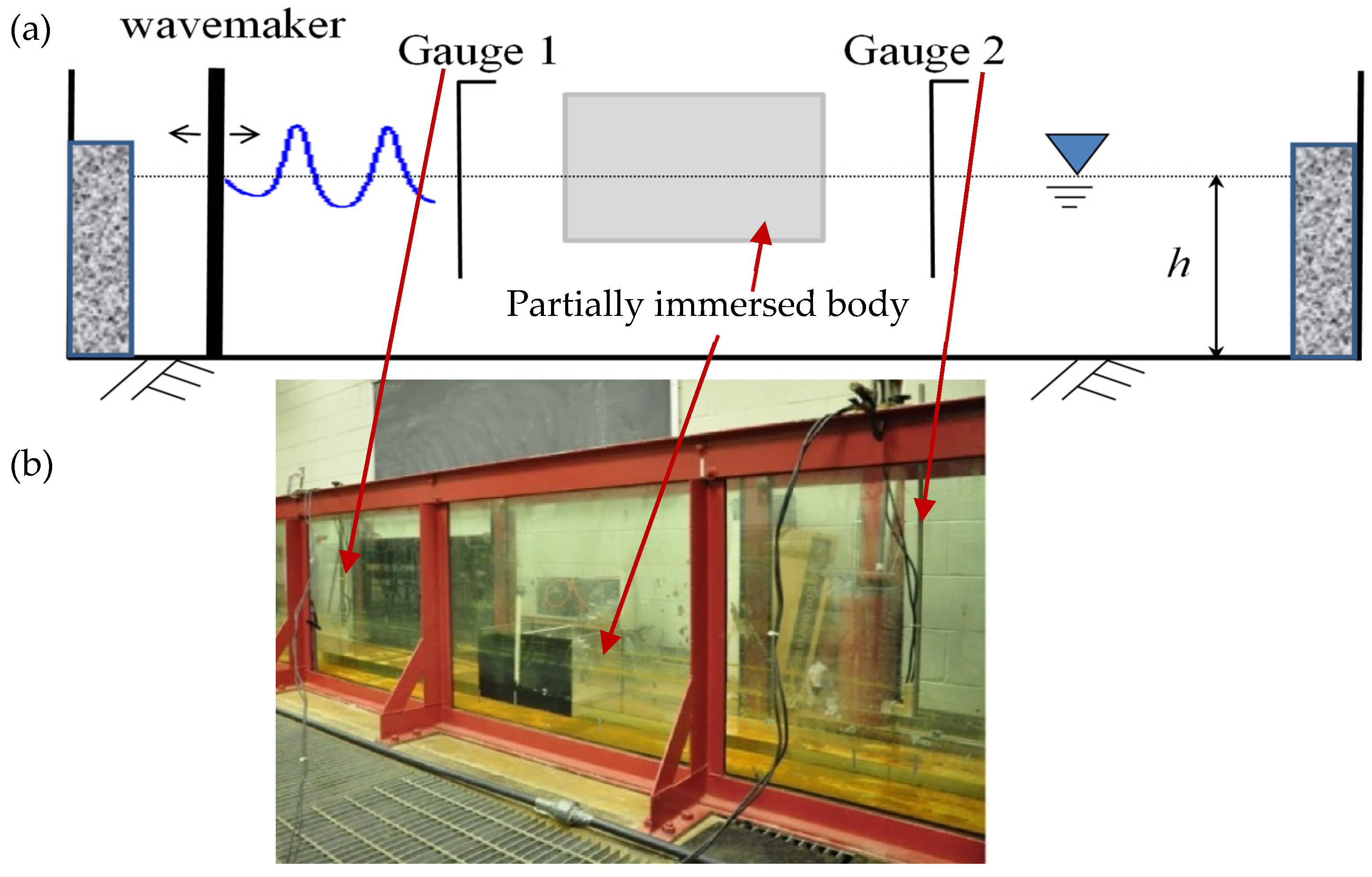
To confirm the solutions of free-surface elevation obtained from the present CAN model, laboratory measurements were performed in a glass-walled wave tank with dimensions of 762 cm (25 ft) in length, 30.48 cm (1 ft) in width, and 91.44 cm (3 ft) in height. A sketch and a photo showing the experimental setup in the wave flume are presented in Figure 2.

A Tolomatic linear-actuator-controlled piston-type wavemaker was used at one end of the tank to generate the desired cnoidal waves. The accuracy of the actuator motion is 3.175 × 10⁻⁴ cm. Porous-type structures were placed at the other end of the tank to eliminate waves reaching there. Two resistance-type wave gauges (Gauge 1 and Gauge 2) were installed in the flume to record the wave elevations at the locations of interest. The data-sampling rate is 20 HZ. The wave gauges were calibrated carefully in which a good linear correlation with the coefficient of determination $R^2$ = 0.998 between the voltage and water surface level was achieved. One gauge was installed in between the wavemaker and body for measuring the incident and reflected waves while the other one was placed behind the body to record the transmitted waves. The bodies with three different sizes (or thicknesses), namely 4, 6, and 10 times of the water depth, were made of plexiglass. For the model tests, the water depth was set at 7.62 cm (0.25 ft).

The position of a moving wavemaker determines the desired wave to be generated. For nonlinear shallow-water waves, the wave paddle position $X(t)$ can be described by the following mass conservation equation [26]:

$$\frac{dX(t)}{dt}=\frac{c\mathsf{\zeta }(X(t),t)}{1+\mathsf{\zeta }(X(t),t)},$$

(36)

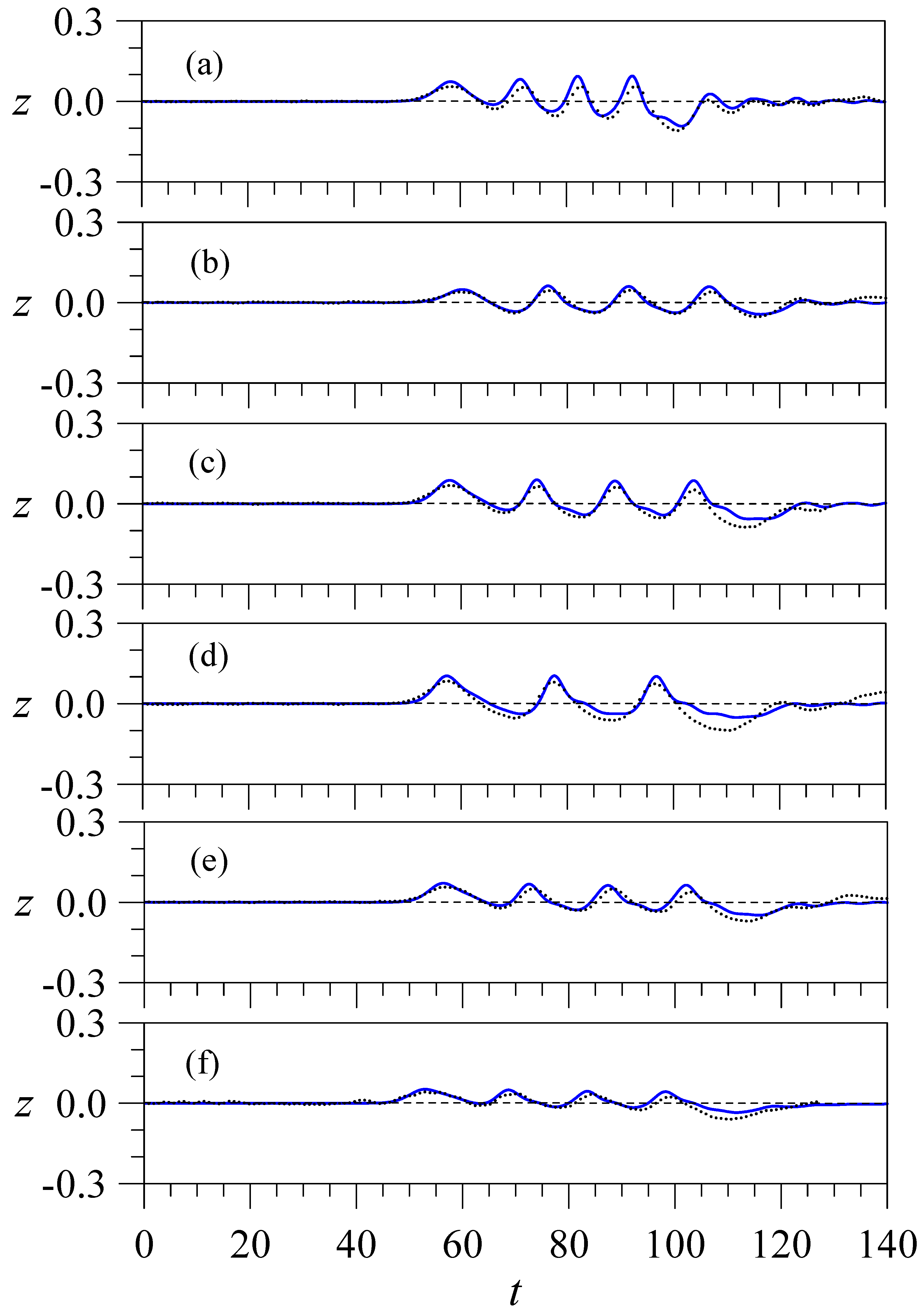
By solving Equation (36) with the input of a given cnoidal wave condition (Equation (11)), the positions calculated can be used to control the motion of the wavemaker. Due to the length limitation of the wave tank, waves covering four wave periods were generated for data collection. As waves were generated from a quiescent water surface condition, a smaller leading wave front followed with three fully developed cnoidal waves was observed (see Figure 3).

Various parameters that affect the outcomes of the reflected and transmitted waves were tested. Waves with wave heights ranging from $\alpha =$ 0.15 to 0.3 and wave lengths of $\lambda$ = 10, 15, and 20 were generated to examine the effect of wave conditions. The effects of structural thickness and submerged depth (or draft) on transmitted waves were also examined. The thicknesses of the tested bodies include L^* = 30.48, 45.72, and 76.2 cm (or in dimensionless form, $L=L^{*}/h_0^{*}=$ 4, 6, and 10). Each tested body was also placed at two different draft positions namely $h_1^{*}=$ 1.524 cm and 3.81 cm (or in dimensionless values, $h_1=$ 0.2 and 0.5) for the lab tests.

6. Results

The results using the present CAN model for simulating the encountering process between a cnoidal wave and a fixed partially immersed body are presented in this section. Model validation was carried out to compare the computed solutions with the laboratory measurements collected from this study and results from the 2D fully nonlinear wave model (FNWM). For the convenience of showing the model and experimental results, the dimensionless values of all physical variables are presented.

6.1. Model Validation with Comparisons between Computed and Recorded Wave Profiles

6.1.1. Incident and Reflected Waves

For validating model performance, the computed time variations of the incident and reflected waves under various wave and structural conditions were first compared with the measured data. The domain length was set as 140 with x = −73 and x = 67 denoting the coordinates at the left and right domain boundaries, respectively. The dimensionless grid size (Δx) of 0.25 was used for the outer-region calculation. The discussion of the mesh refinement for justifying the use of the selected grid size is given in Appendix C. The x coordinates of the left interface (grid index of N1) and the right interface (grid index of N2) vary depending on the thickness of the body. For example, when the set body thickness (L) is equal to 4, the x coordinates arranged at the N1 and N2 locations are, respectively, x = −2 and x = 2. In this case, the number of grid points for the upstream region (from x = −73 to x = −2 or from the left domain boundary to N1) is 285, including the left interfacial point. For the downstream region (from x = 2 to x = 67 or from N2 to the end boundary), the number of grid points is 261, including the right interfacial point. With Δx = 0.25, the number of grid points per wave length varies with the input of the wave length of a selected incident wave. For a λ = 15 wave, 61 grid points can be assigned to cover a wave length of that wave. When the wave length increases to λ = 20, the number of grid points increases to 81. For the time step Δt, it was set as 0.1. It is noted due to the limitation of wavetank length, the comparisons were made reliably within four wave periods, including the frontal wave.

The comparison results, which include the simulated incident and reflected wave profiles from the CAN model and measured data, are presented in Figure 3. The dimensionless root-mean-squared errors (RMSEs) for the six cases compared are also provided in Figure 3 to reflect the model performance. According to all data collected in the wavetank measurements, the comparisons cover the cases with various inputs of wave parameters (α and λ), body thickness (L), and draft ($h_1$) for model validation. As shown in Figure 3a, the comparison results are based on the input parameters of α = 0.3, λ = 10, $h_1$ = 0.2, and $L$ = 4. In this case, the Ursell number, U_r, which is defined as $U_r=H^{*}{\lambda }^{{*}^2}/h^{{*}^3}=\alpha {\lambda }^2$ is equal to 30. The results from Figure 3a indicate that the wave profiles predicted by the present model are in reasonably good agreement with the experimental measurements. It can be seen that the wave peak and trough of theoretically input incident waves are slightly higher than the measured ones. However, the temporal variations of the wave elevation match nicely. In terms of the reflected waves at time t > 120, the agreement is generally reasonable. In Figure 3b, the incident wave height and wave length are set, respectively, as α = 0.15 and λ = 15 (U_r = 33.75), while the draft and body thickness remain as $h_1$ = 0.2 and L = 4. In this case, with a smaller incident wave height, the model calculated incident and reflected wave profiles, including wave peak and general wave trend, agree well with the measured data.

With an increased draft and a longer wave length when compared to the input parameters considered in Figure 3a, for the case of α = 0.3, λ = 15, $h_1$ = 0.5, and L = 4 (U_r = 67.5), the results as illustrated in Figure 3c suggest that the agreement level between model and experimental results is similar to those given in Figure 3a. However, with an increased body draft, a bigger wave is reflected back causing the wave height of the reflected waves (as shown in Figure 3c) to be greater than that given in Figure 3a. When increasing the wave length further from λ = 15 to λ = 20, with α = 0.3, $h_1$ = 0.5, and L = 4 (U_r = 120), the comparisons of the incident and reflected wave profiles are presented in Figure 3d, where an acceptable agreement is noticed. In particular, the wave peak of incident waves is well predicted. With the inputs of α = 0.3, λ = 15, and $h_1$ = 0.5 (U_r = 67.5), the results presented in Figure 3e,f are based on the body thickness of L = 6 and L = 10, respectively, to show the effectiveness of body size on the incident and reflected waves. Again, the incident and reflected wave solutions obtained from the present CAN model agree reasonably well with the measured data. In general, the wave crests from the measurements are slightly less than those from the model predictions and the wave troughs depress a little more than the model solutions. However, the temporal variations between the present model results agree well with the measurements. Overall, the average RMSE between the predicted incident/reflected wave elevations and experimental data for the six cases simulated is about 0.0283. When compared to the incident wave height of 0.3, the error is about 9.4%. Those differences are the reflection of the negligence of the effects of fluid viscosity, energy dissipation, and the additional wave damping as the waves propagate through a partially submerged body. The cases with a longer wave length, smaller incident wave height, smaller draft, and smaller body thickness produce relatively smaller errors in wave peak and general wave profile predictions.

6.1.2. Transmitted Waves

In terms of transmitted waves, the computed and measured values in time variations are plotted in Figure 4 for comparisons. The input parameters for the six cases as mentioned in Figure 3 are: (a) α = 0.3, $\lambda$ = 10, h₁ = 0.2, L = 4, (b) α = 0.15, $\lambda$ = 15, h₁ = 0.2, L = 4, (c) α = 0.3, $\lambda$ = 15, h₁ = 0.5, L = 4, (d) α = 0.3, $\lambda$ = 20, h₁ = 0.5, L = 4, (e) α = 0.3, $\lambda$ = 15, h₁ = 0.5, L = 6, and (f) α = 0.3, $\lambda$ = 15, h₁ = 0.5, L = 10. The RMSEs of the computed values are also provided to confirm the model performance in predicting the transmitted waves. Comparisons of the transmitted wave profiles from the present CAN model and measured data are in reasonable agreement. Well-matched results are noticed for cases with smaller incident wave height as indicated in Figure 4b. It is noted that the transmitted waves from the experimental data travel a little bit slower than those obtained from the present model simulations. Additionally, the transmitted wave peak from model predictions, in general, is slightly over-estimated. Those small discrepancies are believed to be caused by the energy losses initiated from the solid surfaces of the channel and body, fluid viscosity, and induced eddies. For the six cases simulated, the average RMSE between the predicted transmitted wave elevations and measured data is about 0.0166. Again, when compared to the incident wave height of 0.3, the average error is about 5.5%, which is smaller than that made to the predictions of the incident and reflected waves in the region upstream of a partially immersed body.

6.2. Comparisons with Results from a Fully Nonlinear Wave Model

Here, we further compare the results, especially the induced horizontal and vertical forces, obtained from the CAN model presented in this paper with those from a fully nonlinear wave model (FNWM) developed by Chang et al. [13]. In this fully nonlinear wave model, the incident cnoidal wave condition was input into the domain from the left open boundary as a wavemaker that is specified with a motion given by Equation (36). Firstly, two cases are selected to compare the wave profiles calculated from the present CAN model with those from FNWM. Both cases are under the conditions α = 0.3, h₁ = 0.5, and L = 4 but with different wave lengths. The comparison plots shown in Figure 5 and Figure 6 are for the cases λ = 15 and 20, respectively. As a reference, the experimentally measured data from the present study are also plotted for comparisons.

For the results presented in Figure 5, including the leading wave front, four waves entered the computational domain from the left open boundary to model the wave propagation and subsequent wave encountering process with the body. The results showing the incident and reflected waves are presented in Figure 5a and Figure 6a, respectively. As can be seen in Figure 5a and Figure 6a, consistently matched wave profiles among the results obtained from the CAN model, FNWM, and measured data can be noticed. The peaks of the incident waves from the CAN model are slightly higher than those from FNWM. However, for the reflected waves, the solutions of the FNWM and CAN model are in close agreement. Overall, the FNWM’s results fit slightly better than those from the CAN model when compared to the experimental data. For the transmitted waves, as a result of the blockage effect caused by the partially immersed body, their wave heights are less than half of the incident wave heights (see results shown in Figure 5b and Figure 6b). The results from the CAN model and FNWM again match closely with the measured transmitted wave elevations. Compared to the experimental data, the FNWM generated wave profiles give slightly improved predictions in wave trough and crest than those from the CAN model.

For the total horizontal and vertical forces exerted by a cnoidal wave on a partially immersed body, according to Equations (33) and (34) in the dimensionless form, both the hydrostatic and hydrodynamic contributions are included in the calculation. The calculated horizontal and vertical forces from the present CAN model are compared with those from the FNWM. We used the same case as presented in Figure 5 for the wave profile results to show the force comparisons. The time variations of the dimensionless horizontal and vertical forces computed from the present CAN model under the conditions L = 4 and h₁ = 0.5 are illustrated, respectively, in Figure 7a,b to compare to the results obtained from the FNWM. The wave input parameters are α = 0.3 and λ = 15. As seen in Figure 7a, the present CAN model is found to be able to produce closely matched horizontal forces with the results from the fully nonlinear wave model. For the vertical force, as shown in Figure 7b, the results from the present CAN model are in acceptable agreement with those from the FNWM simulations, including the time variation of the force values. The CAN model predicted values of force peak or trough are shown to be slightly greater than the FNWM results. The force comparisons presented in Figure 7 suggest that the present CAN model can effectively provide reasonable predictions on the cnoidal wave-induced horizontal or vertical force after encountering a partially submerged rectangular body.

6.3. Effects of Body Draft and Thickness on Transmission Coefficient and Horizontal Force

The effect of body draft on the transmitted waves is examined with a plot showing the variations of transmission coefficient (C_t) under the conditions of different values of the body draft (h₁). The transmission coefficient (C_t) was calculated as the ratio of the transmitted wave height versus the incident wave height. For a given incident cnoidal wave with wave height α = 0.3 and wave length λ = 15, the varying trends of transmission coefficient (C_t) versus body draft (h₁) under various body thickness conditions are presented in Figure 8. The body thickness conditions include L = 2, 4, and 8. It can be seen that the transmission coefficient decreases with an increase in body draft. As the draft of the body increases, a decrease in the opening beneath the body places more limits on the fluid motion transmitting through the body. For the case with a dimensionless draft of 0.1 and L = 4, the transmitted wave height can reach about 60% of the incident wave height. When the draft increases to 0.8 (or opening in 20% of the water depth), the transmitted wave height is reduced to about 20% of the incident wave height. When considering the limiting case, where the body completely separates the two outer regions, the transmission coefficient can be seen approaching zero. The results in Figure 8 also show that with an increase in the thickness of the body, the transmission coefficient decreases. The effect of body draft on the horizontal force is illustrated in Figure 9 with a sequence of time-series plots of horizontal force for various body draft conditions. Again, the incident cnoidal wave conditions are set as α = 0.3 and λ = 15. The body thickness is fixed as L = 4 while the draft condition varies from h₁ = 0.1 to h₁ = 0.9. Clearly, it can be seen that the peak value of the positive horizontal force increases as the body draft increases. A similar effect of body draft on the negative horizontal force can also be concluded.

7. Conclusions

This paper introduced a combined analytical and numerical (CAN) model to simulate the scattering of a cnoidal wave by a partially immersed stationary 2D body. The model performance was examined by comparing the simulated wave elevations with the measured data. The computed horizontal and vertical forces on the body were compared with the results obtained numerically from a 2D fully nonlinear wave model (FNWM) for validation. The proposed approach integrated the inner analytical solutions with the outer numerical results through the formulations derived from the matching conditions set at the interfaces that separated the interior domain beneath a partially immersed body and the exterior domain of the upstream and downstream of the body. When simultaneously solving the derived matching equations with the outer finite-difference numerical formulations of the Boussinesq equations, the velocity potentials, free-surface elevations, and wave forces along the horizontal and vertical directions can be effectively determined. Wavetank tests for selected wave conditions with a partially immersed body of varying thickness and draft were carried out to record the incident, reflected, and transmitted waves for verification of the model predictions.

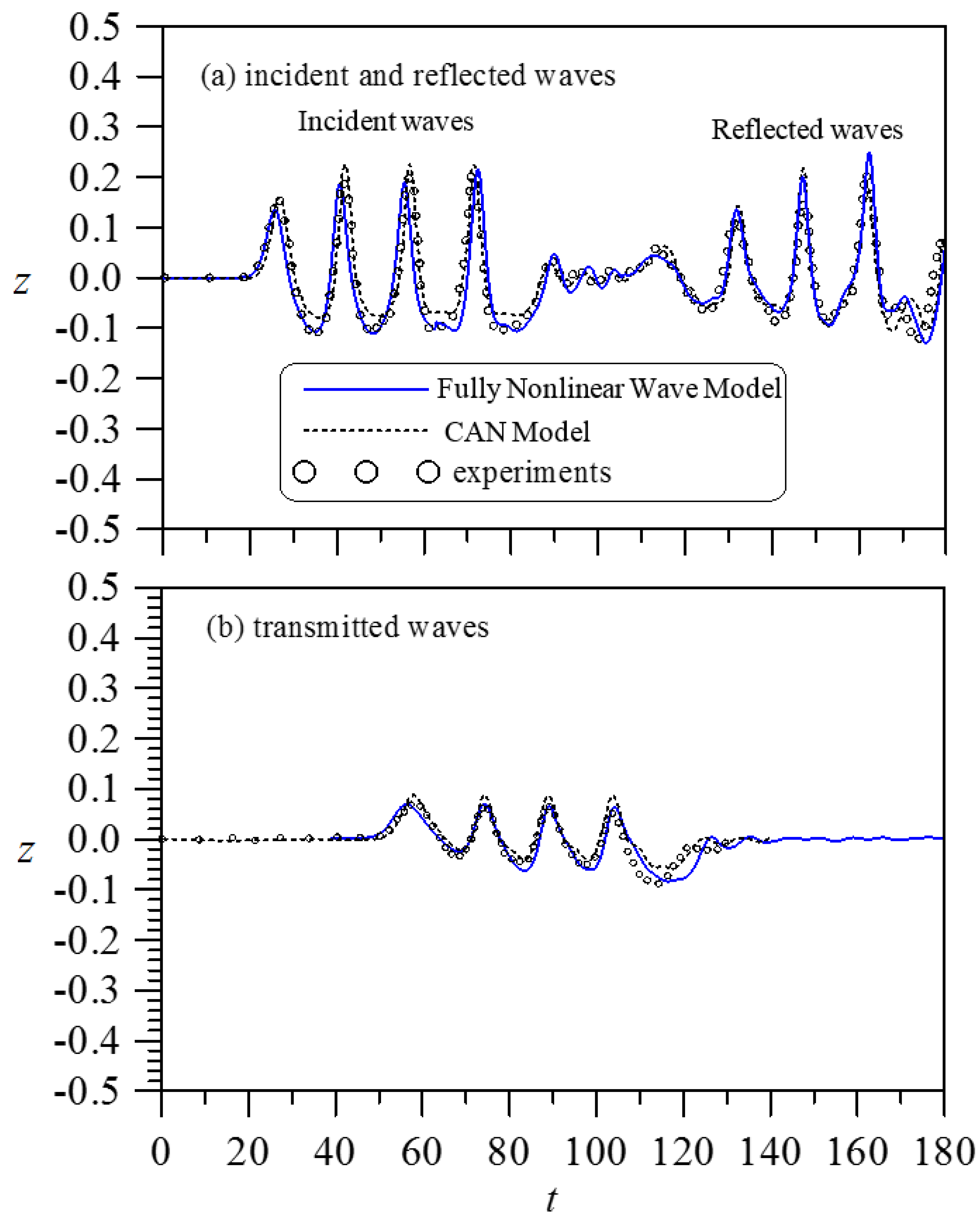
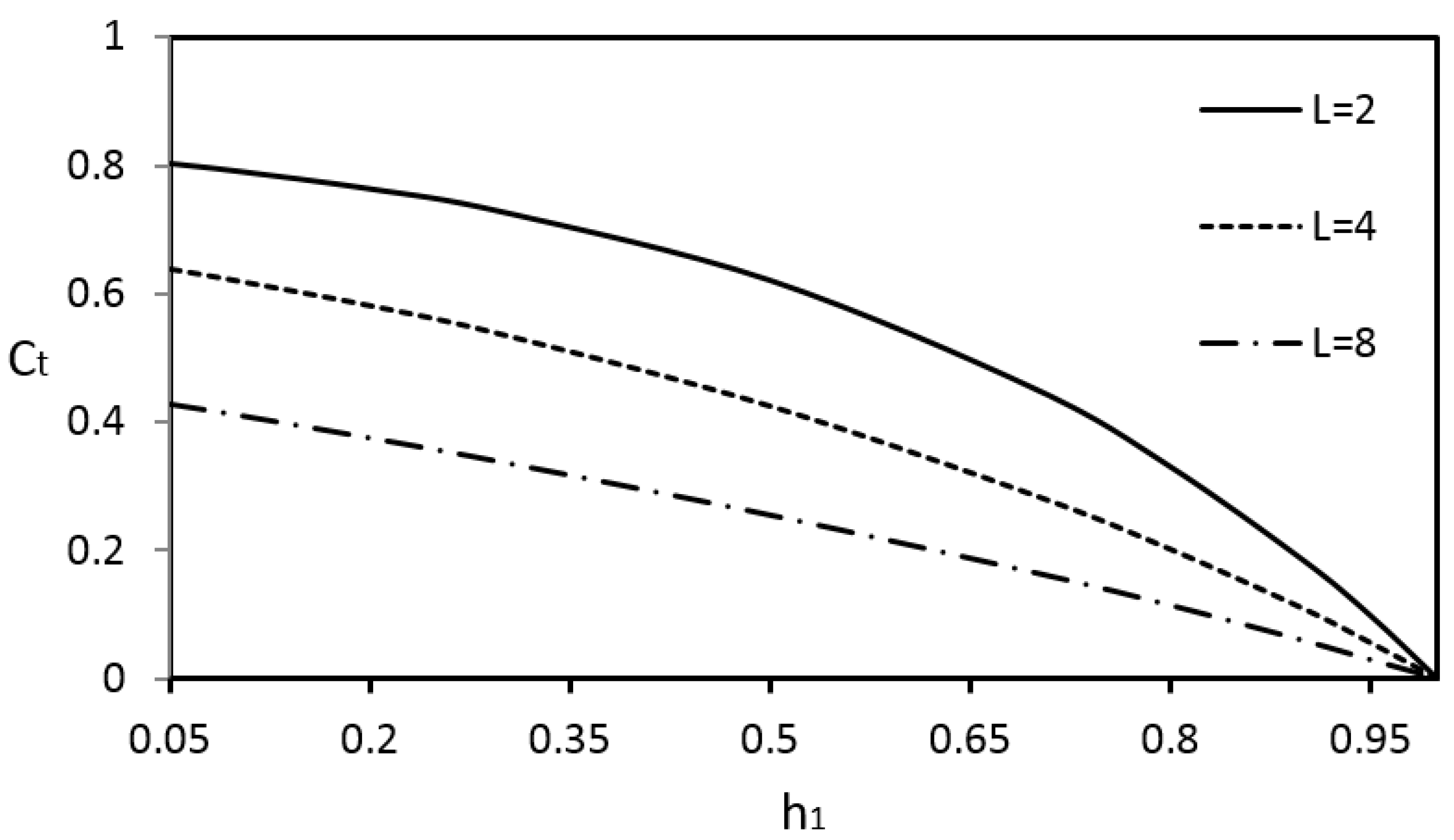
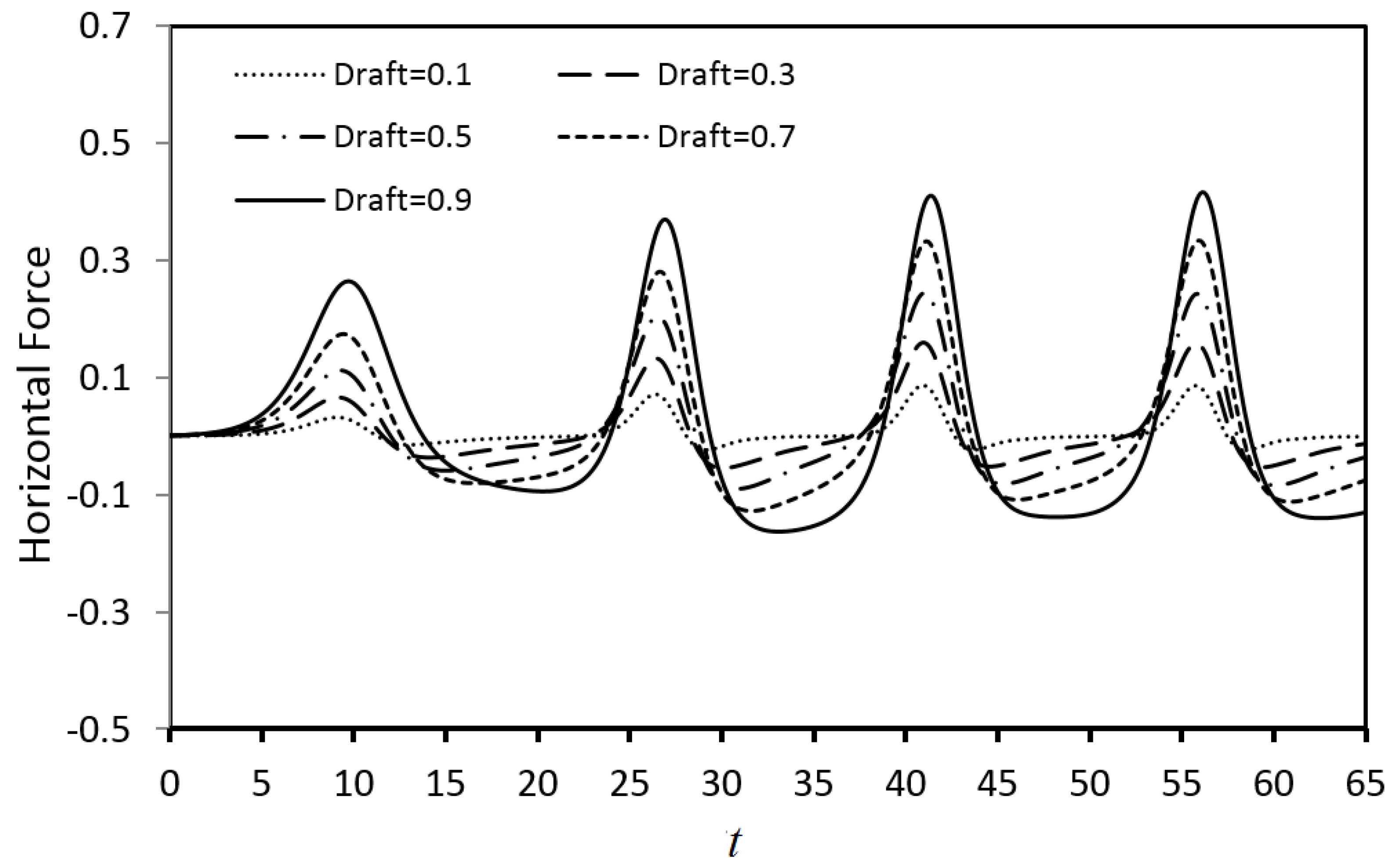
It was found that both the reflected and transmitted wave profiles obtained from the present CAN model agree reasonably well with the measured data. In general, the reflected or transmitted wave peak was slightly over-estimated due to the negligence of the effects of energy dissipation and fluid viscosity in the model development. The CAN model produced much smaller comparison errors in wave peak predictions when the case of a relatively longer wave length, smaller incident wave height, smaller body draft, or smaller body thickness was considered. The time variations of the cnoidal wave-induced forces were calculated. Due to the limitation of the equipment setup and a relatively small wave tank, the wave forces were not measured. It was found that the horizontal forces computed from the present CAN model matched closely with the results from a fully nonlinear wave model (FNWM). In terms of the vertical forces, the CAN model was able to predict a similar variation trend as those from the FNWM with slightly greater values of the maximum force. Additionally, the proposed CAN model, if applied to a simple parametric investigation, can provide the expected trends in terms of applied forces, wave reflection, and transmission, such as when the body draft or its thickness increases, the transmitted wave height decreases, and the maximum horizontal force increases.

References

1. Mei, C.C.; Black, J.L. Scattering of surface waves by rectangular obstacles in water of finite depth. J. Fluid Mech. 1969, 38, 499–511. [Google Scholar] [CrossRef]
2. Martin, P.A.; Dixon, A.G. The scattering of regular surface waves by a fixed, half-immersed, circular cylinder. Appl. Ocean Res. 1983, 5, 13–23. [Google Scholar] [CrossRef]
3. McCartney, B.L. Floating breakwater design. J. Waterw. Port Coast. Ocean Eng. 1985, 111, 304–318. [Google Scholar] [CrossRef]
4. Drimer, N.; Agnon, Y.; Stiassnie, M. A simplified analytical model for a floating breakwater in water of finite depth. Appl. Ocean Res. 1992, 14, 33–41. [Google Scholar] [CrossRef]
5. Kanoria, M.; Dolai, D.P.; Mandal, B.N. Water-wave scattering by thick vertical barriers. J. Eng. Math. 1999, 35, 361–384. [Google Scholar] [CrossRef]
6. Qiao, W.; Wang, K.H.; Sun, Y. Scattering of water waves by a floating body with two vertically attached porous walls. J. Eng. Mech. 2018, 144, 04017162-1–04017162-13. [Google Scholar] [CrossRef]
7. Kaligatla, R.B.; Prasad, N.M.; Tabssum, S. Oblique interaction between water waves and a partially submerged rectangular breakwater. Proc. Inst. Mech. Eng. M: J. Eng. Marit. Environ. 2020, 234, 154–169. [Google Scholar] [CrossRef]
8. Isaacson, M. Solitary wave diffraction around large cylinder. J. Waterw. Port Coast. Ocean Eng. 1983, 109, 121–127. [Google Scholar] [CrossRef]
9. Wang, K.H.; Wu, T.Y.; Yates, G.T. Three-dimensional scattering of solitary waves by vertical cylinder. J. Waterw. Port Coast. Ocean Eng. 1992, 118, 551–566. [Google Scholar] [CrossRef]
10. Zhong, Z.; Wang, K.H. Modeling fully nonlinear shallow-water waves and their interactions with cylindrical structures. Computers Fluids 2009, 38, 1018–1025. [Google Scholar] [CrossRef]
11. Lu, X.; Wang, K.H. Modeling a solitary wave interaction with a fixed floating body using an integrated analytical-numerical approach. Ocean Eng. 2015, 109, 691–704. [Google Scholar] [CrossRef]
12. Xu, G.; Cai, C.; Deng, L. Numerical prediction of solitary wave forces on a typical coastal bridge deck with girders. Struct. Infrastruct. Eng. 2017, 13, 254–272. [Google Scholar] [CrossRef]
13. Chang, C.H.; Wang, K.H.; Hsieh, P.C. Fully nonlinear model for simulating solitary waves propagating through a partially immersed rectangular structure. J. Coast. Res. 2017, 33, 1487–1497. [Google Scholar] [CrossRef]
14. Chen, Y.H.; Wang, K.H. Experiments and computations of solitary wave interaction with fixed, partially submerged, vertical cylinders. J. Ocean Eng. Mar. Energy 2019, 5, 189–204. [Google Scholar] [CrossRef]
15. Isaacson, M. Shallow wave diffraction around large cylinder. J. Waterw. Port Coast. Ocean Eng. 1977, 103, 69–81. [Google Scholar] [CrossRef]
16. Wang, K.H.; Ren, X. Interactions of cnoidal waves with cylinder arrays. Ocean Eng. 1999, 26, 1–20. [Google Scholar] [CrossRef]
17. Weng, Y.; Xu, X.; Huang, H. Interaction of cnoidal waves with an array of vertical concentric porous cylinders. Appl. Ocean Res. 2016, 58, 21–36. [Google Scholar] [CrossRef]
18. Zhang, J.S.; Teng, B. Numerical study on cnoidal wave run-up around a vertical circular cylinder. Appl. Ocean Res. 2017, 63, 276–287. [Google Scholar] [CrossRef]
19. Tang, C.J.; Lee, T.C. Numerical hybrid grid for cnoidal wave generation and induced separated flow over a wavy bed. J. Eng. Mech. 2014, 140, 06014009-1–06014009-7. [Google Scholar] [CrossRef]
20. Ren, X.; Ma, Y. Numerical simulations for nonlinear waves interaction with multiple perforated quasi-ellipse caissons. Math. Prob. Eng. 2015, 486, 895673-1–895673-14. [Google Scholar] [CrossRef]
21. Jiang, L.; Ren, X.; Wang, K.H.; Jin, K.R. Generalized Boussinesq model for periodic nonlinear shallow water waves. Ocean Eng. 1996, 23, 309–323. [Google Scholar] [CrossRef]
22. Ouro, P.; Juez, C.; Franca, M. Drivers for mass and momentum exchange between the main channel and river bank lateral cavities. Adv. Water Resour. 2020, 137, 103511-1–103511-14. [Google Scholar] [CrossRef]
23. Navas-Montilla, A.; Juez, C.; Franca, M.J.; Murillo, J. Depth-averaged unsteady RANS simulation of resonant shallow flows in lateral cavities using augmented WENO-ADER schemes. J. Comput. Phys. 2019, 395, 511–536. [Google Scholar] [CrossRef]
24. Jiang, L.; Wang, K.H. Hydrodynamic interactions of cnoidal waves with a vertical cylinder. Appl. Ocean Res. 1995, 17, 277–289. [Google Scholar] [CrossRef]
25. Sarpkaya, T.; Isaacson, M. Mechanics of Wave Forces on Offshore Structures; Van Nostrand Reinhold Co.: New York, NY, USA, 1981. [Google Scholar]
26. Goring, D.G. Tsunamis-The Propagation of Long Waves onto a Shelf. Ph.D. Thesis, California Institute of Technology, Pasadena, CA, USA, 1978; 356p. [Google Scholar]
Figure 1. A schematic diagram showing the fluid domains for the analyses of an incident cnoidal wave encountering a fixed and partially submerged rectangular body.
Water 14 00318 g001
Figure 2. (a) Laboratory diagram showing the measurements of wave elevation at Gauge 1 for the incident and reflected waves and Gauge 2 for the transmitted waves. (b) Photo showing a partially submerged body and wave gauges in the wave tank.
Water 14 00318 g002
Figure 3. Comparisons of time variations of incident and reflected waves between the present CAN model solutions (solid-blue lines) and experimental data (black-dotted lines) for cnoidal waves encountering with a partially immersed body with various input parameters, (a) α = 0.3, λ = 10, h1 = 0.2, L = 4, (RMSE = 0.0211), (b) α = 0.15, λ = 15, h1 = 0.2, L = 4, (RMSE = 0.00856), (c) α = 0.3, λ = 15, h1 = 0.5, L = 4, (RMSE = 0.02), (d) α = 0.3, λ = 20, h1 = 0.5, L = 4, (RMSE = 0.0683), (e) α = 0.3, λ = 15, h1 = 0.5, L = 6, (RMSE = 0.0265), and (f) α = 0.3, λ = 15, h1 = 0.5, L = 10, (RMSE = 0.0252).
Water 14 00318 g003
Figure 4. Comparisons of time variation of transmitted waves between the present CAN model solutions ((solid-blue lines) and experimental data (black-dotted lines) for cnoidal waves encountering a partially submerged body for various input parameters, (a) α = 0.3, λ = 10, h1 = 0.2, L = 4, (RMSE = 0.0149) (b) α = 0.15, λ = 15, h1 = 0.2, L = 4, (RMSE = 0.00753) (c) α = 0.3, λ = 15, h1 = 0.5, L = 4, (RMSE = 0.034) (d) α = 0.3, λ = 20, h1 = 0.5, L = 4, (RMSE = 0.02) (e) α = 0.3, λ = 15, h1 = 0.5, L = 6, (RMSE = 0.0122) and (f) α = 0.3, λ = 15, h1 = 0.5, L = 10 (RMSE = 0.011).
Water 14 00318 g004
Figure 5. Comparisons of the incident and reflected wave profiles in subplot (a) and transmitted wave profiles in subplot (b) obtained from the present CAN model, a FNWM, and measured data for a cnoidal wave encountering a partially submerged body with h1 = 0.5, L = 4. The incident cnoidal wave conditions are α = 0.3 and λ = 15.
Water 14 00318 g005
Figure 6. Comparisons of the incident and reflected wave profiles in subplot (a) and transmitted wave profiles in subplot (b) obtained from the present CAN model, a FNWM, and measured data for a cnoidal wave encountering a partially submerged body with h1 = 0.5, L = 4. The incident cnoidal wave conditions are α = 0.3 and λ = 20.
Water 14 00318 g006
Figure 7. Comparisons of time variations of the dimensionless horizontal force in (a) and dimensionless vertical force in (b) obtained from the present CAN model and FNWM under the wave and structural conditions of α = 0.3, λ = 15, L = 4, and h1 = 0.5.
Water 14 00318 g007
Figure 8. Variations of transmission coefficient (Ct) versus body draft (h1) for the cases of L = 2, 4, and 8 using the incident wave conditions of α = 0.3, λ = 15.
Water 14 00318 g008
Figure 9. Time-series plots of horizontal force for various body draft conditions using the incident wave conditions of α = 0.3 and λ = 15. The body thickness is set as L = 4.
Water 14 00318 g009
Publisher’s Note: MDPI stays neutral with regard to jurisdictional claims in published maps and institutional affiliations.