Predicting Discharges in Sewer Pipes Using an Integrated Long Short-Term Memory and Entropy A-TOPSIS Modeling Framework

Abstract

Predicting discharges in sewage systems play an essential role in reducing sewer overflows and impacts on the environment and public health. Choosing a suitable model to predict discharges in these systems is essential to realizing these aforementioned goals. Long Short-Term Memory (LSTM) has been proposed as a robust technique for predicting discharges in wastewater networks. This study explored the potential application of an LSTM model to predict discharges using 3-month data set in a sewer network in Ålesund city, Norway. Different sequence-to-sequence LSTMs were investigated using various input and output datasets. The impact of data aggregation (10-min and 30-min intervals) was examined and compared to original sensor data (5-min intervals) to evaluate the performance of the LSTM model. The results show that 50-neuron LSTM architecture performed better (MAPE = 0.09, RMSE = 0.0008, R² = 0.8) in predicting discharges for the study area. The study indicates that using the same sequence length for the prior and the forecast can improve the effectiveness of the LSTM model. Based on the results, using a 10-min aggregated discharge dataset reduces energy consumption, transmission bandwidth, and storage capacity. Additionally, it improves prediction performance compared to an original 5-min interval data in Ålesund city.

1. Introduction

Pipelines, manholes, and pumps mainly characterize wastewater and stormwater drainage systems. Wastewater pipelines collect and transport wastewater from households and industries, while stormwater pipes mainly collect and transport runoffs from rainfall and snowmelt [1]. In many European countries, there are combined sewer systems (CSSs), designed and built for the collection and transport of wastewater and stormwater. For instance, in Norway, sewers comprising of CSSs and stormwater drains account for 35,900 km and 15,700 km, respectively, of the entire sewer system [2]. Rapid urbanization combined with increased precipitation due to climate change and low investments in the rehabilitation of aging CSSs have resulted in the increased incidence of combined sewer overflows (CSOs) in Norway [3,4,5]. A study by Nilsen et al. [5] revealed a significant relationship between the volume of CSOs in the sewer network in Oslo and flood events.

A study has also shown the utility of forecasting in developing risk analysis models for the optimal operations of a reservoir to reduce flood incidents [6]. According to the International Committee for Weights and Measures, flows in wastewater pipes remain a significant challenge [7], and increased sediment deposition with limited self-cleansing has often led to the reduction of the capacity of wastewater pipes [8,9].

The occurrence of CSOs not only pollutes the natural environment but can also result in deleterious public health impacts [10]. For instance, hazardous chemicals, such as mercury, zinc, lead, and chromium, usually present in stormwater/wastewater can affect fauna and flora when discharged untreated into the environment [1]. There are currently no robust early warning systems in many cities in Europe in general, and Norway in particular, designed to reduce the incidence of CSOs and mitigate the associated environmental and public health risks. According to Hanssen-Bauer et al. [11], precipitation is expected to increase by 20% in the next 80 years. This will result in further stresses on CSSs and major CSOs if the current rate of investments in CSSs remains the same. In the last decade, there has been a renewed interest in forecasting discharges in sewer and wastewater networks to help utilities prepare for the adverse impact of overflows and develop measures to manage these drainage systems more effectively. Wang et al. [12] highlighted the role of long-term discharge forecast in environmental protection, effective management of drought, and the optimization of hydraulic system operations. The result showed that Wastewater Treatment Plants (WWTPs) operate more effectively when discharges in the networks are known with some degree of certainty [13,14].

For forecasting discharges in stormwater/wastewater pipe systems, municipalities in Norway are investing in sensors installations and IoT systems for the real-time collection of discharge data from their wastewater/stormwater water pipe network. The aim is to develop a real-time predictive discharge modeling framework using big data to mitigate the incidence of CSOs, reduce impacts on the environment, and better plan investment prioritization for their wastewater/stormwater pipe networks. For such a real-time predictive discharge modeling framework to be useful, there is a need for an appropriate modeling algorithm that (a) accounts for the variability and sensitivity in the discharge data from installed sensors, (b) has a high predictive performance with a reasonable a-prior time lag, and (c) is cost-effective through data aggregation.

Therefore, developing a real-time predictive modeling framework based on IoT and big data to account for discharges in CSSs is critical. This will enable decision makers to prepare in advance for possible CSOs and develop the necessary mitigation measures to reduce any adverse impacts.

Traditionally, hydraulic models have been used to forecast discharges, and these models have achieved some appreciable performance [15,16,17]. However, most of these models do not accurately forecast water levels compared to observations [15]. In addition, the anticipated real-time capacity of hydraulic models has been limited to extreme flood events because of uncertainties associated with input parameters [16]. Zhang et al. [14] showed that hydraulic models are unsuitable for time-series discharge forecasts because of their computational burden, numerous input parameters, and requirement for detailed information about the system, which is most often non-existent. In general, good foreknowledge of the sewer network is required to implement the hydraulic models. The calibration, simulation, and operation of these models are manual and time consuming [13].

In an attempt to address some of the deficiencies of physical-based hydraulic models, statistical models for time-series prediction have been adopted in previous studies. Box et al. [18] introduced Auto Regressive Moving Average (ARMA) and Auto-Regressive Integrated Moving Average (ARIMA) for time-series forecasting, which has become one of the most utilized statistical methods in hydrological forecasting [19]. Valipour [20] presented a comparative study of various statistical models, such as applied Auto-Regressive (AR), Moving Average (MA), ARMA, and ARIMA, for time-series analysis and forecasting of the monthly reservoir inflow of the Dez dam. A statistical method based on the canonical correlation analysis method was also presented by Uvo and Graham [21] to forecast seasonal runoff in northern South America. In addition, some studies have used hybrid statistical–hydrological approaches to forecast seasonal discharge streamflow [22], but these approaches require significant efforts for the hydrological simulation [23]. Other hybrid methods based on the combination of ARIMA and different algorithms, such as Genetic Programming (GP) [24,25], Artificial Neural Networks (ANNs) [26], Support Vector Machine (SVM) [27], and Elman’s Recurrent Neural Networks (ERNN) [28], have been used to improve time-series prediction performance. Even though statistical and statistical–hydrological models have presented another frontier for discharge prediction, they are most often plagued by substantial inefficiencies. Most statistical models fail to capture the complex nonlinear dynamics of sewer discharges [24,29] and also require foreknowledge of discharge distributions [30].

Deep learning algorithms based on Artificial Neural Networks (ANN) have been recommended for processing sequential data or time-series prediction [31,32,33]. Among them, Recurrent Neural Networks (RNN) has been shown to be an effective model for time-series forecasting since this model can “remember” prior information and has been effectively applied for forecasting sequential and time-series data [34]. In time-series forecasting, historical data for an extended period plays a vital role in accurate prediction because the predicted values can be determined based on their patterns in the past [35]. However, one limitation of RNN is that it is unable to accurately learn some exceptionally long period dependencies [36,37]. The Long Short-Term Memory (LSTM) network was proposed to deal with this problem [38]. LSTM was introduced by Hochreiter and Schmidhuber [39] as a particular type of RNN [40]. This structure also helps the LSTM network “learn” long-term dependencies in data [41]. LSTM has found application in finance and production forecast [42,43] but not so much in hydrological time-series prediction of discharges in wastewater and stormwater drainage systems. Therefore, the effectiveness of LSTM should be further investigated to reach reasonable conclusions. For instance, Jenckel et al. [40] showed that an inappropriate input sequence length would reduce LSTM’s understanding/learning ability, as it often groups indistinguishable variables into clusters, and this does not improve predicting performance. This study assessed the effects of input sequence on the LSTM model’s predicting ability and proposed a sensitive LSTM architecture and input sequence to predict discharges in a combined sewer pipeline.

Additionally, there is the need to explore data frequency or data aggregation and its impact on predicting discharges in sewer networks using LSTM. Extremely high-frequency data exhibit too much noise to the extent that there could be no clear pattern for the LSTM models to learn. Too many or too few data are known to result in confusion, lack of clarity, and misunderstanding [44]. Effective data aggregation could potentially reduce the cost of operating Supervisory Control and Data Acquisition (SCADA) networks since energy usage, data storage, and bandwidth would be reduced if it is established that aggregated data provide similar or better forecast accuracy. Therefore, it is crucial to explore the capability of LSTMs under these conditions and recommend appropriate architecture, sequence length, and optimal data aggregation strategy to enhance the prediction of discharges in drainage systems.

The overall aim of this study is to predict discharges in the sewer network using an integrated LSTM and entropy-A-TOPSIS modeling framework. The specific objectives are to (a) explore different LSTM architecture for predicting discharges in the sewer network using the sequence-to-sequence approach, (b) determine the optimal LSTM architecture using the entropy A-TOPSIS method, and (c) assess the effect of data aggregation on the performance of the A-TOPSIS-inspired LSTM architecture.

2. Materials and Methods

2.1. Study Area and Data Used

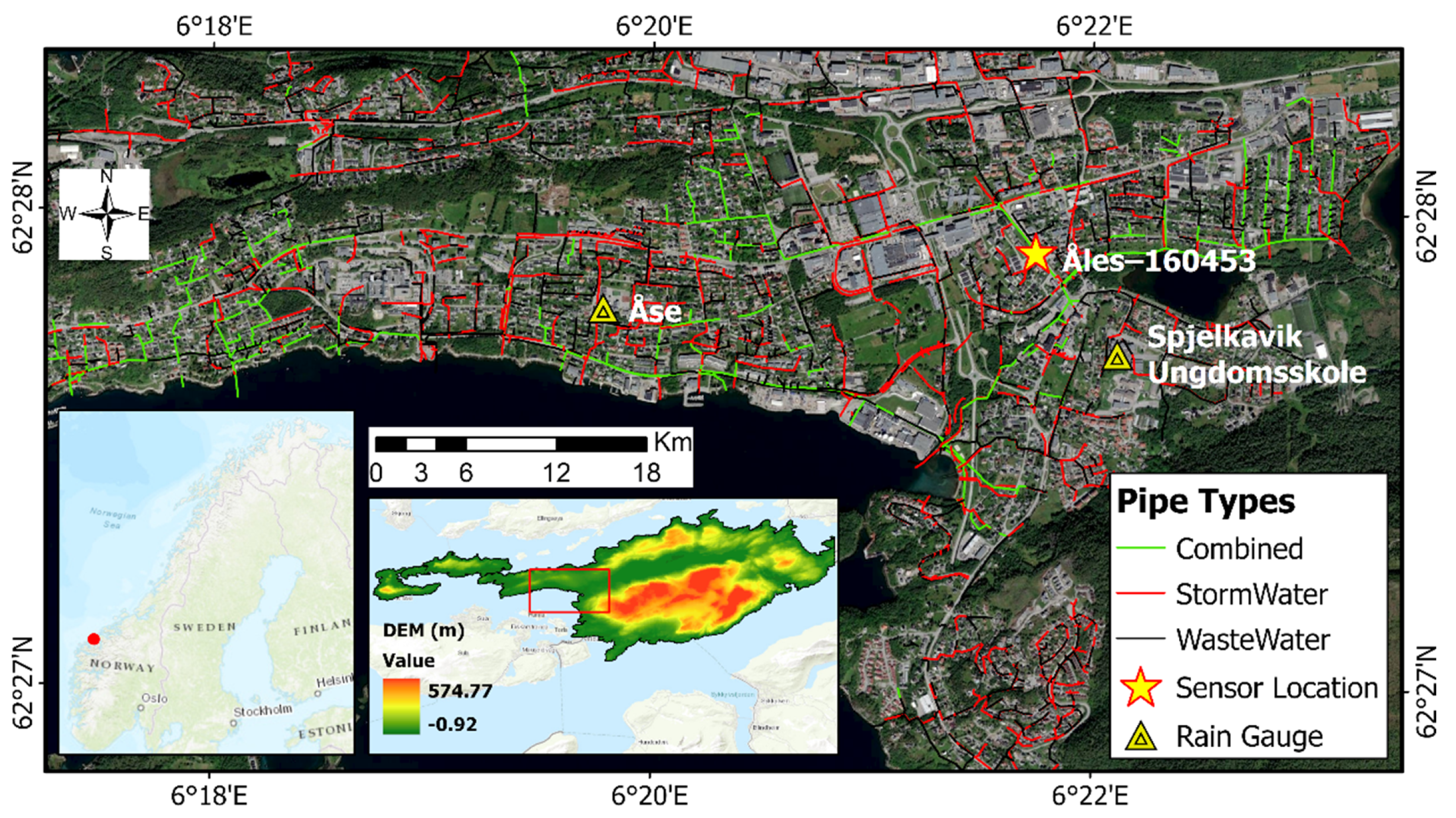
2.1.1. Description of the Study Area and Sensors Installation

The study was undertaken in Ålesund city, which is located along the West Coast of Norway. The city has a population and an area of approximately 66,100 and 633.6 km², respectively [45]. Ålesund experiences high precipitation throughout the year, with an annual average rainfall of 2100 mm [46]. In the driest month (May) of the year, the rainfall averages 104 mm, while the highest rainfall occurs in December, with an average of 230 mm. This rainfall regime results in significant stress on sewer networks, with resultant CSOs.

The drainage network in Ålesund consists of about 37,088 pipes with a total length of 836 km. The total length of wastewater, stormwater, and combined pipes is approximately 417 km, 313 km, and 106 km, respectively. A part of the drainage network in the city is shown in Figure 1. In the Spjelkavik area of the city, flow sensors were installed in the stormwater/wastewater pipe networks for the real-time collection of discharge data. In addition to the flow sensors, a total of two rain gauges were installed to account for precipitation (Figure 1). In this study, a combined wastewater pipeline was selected based on the available dataset. The combined sewer pipeline is located in an area with a great deal of commercial centers and residential buildings with the potential of being affected by combined sewer overflows.

2.1.2. Data Collection and Transmission

Univariate time-series discharge data in the selected wastewater/stormwater pipe were recorded at a time interval of 5-min by the installed flow sensor and transmitted to a cloud-based platform (Regnbye.no) via an IoT system. The data were collected from 14:50:00 (8 September 2020) to 11:45:00 (14 December 2020), resulting in 27,900 distinct data points. Data from the rain gauges in the area were also collected at an interval of 5-min and transmitted to the same platform.

The platform deployed by Rosim AS has three different layers: sensing layer, network layer, and application layer [47]. Sensors and rain gauges are situated in the sensing layer, which continuously receives data (including level and velocity of water in pipes) and transmits them through wireless communication protocols in the network layer. The processing and visualization of the data take place in the application layer [13,47].

2.2. Proposed LSTM Architecture for Predicting Discharges in Sewer Pipes

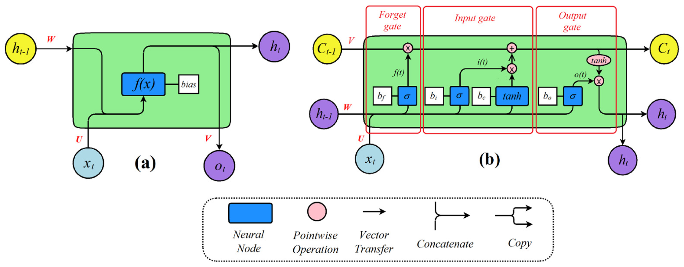
2.2.1. Long Short-Term Memory

LSTM networks have a similar structure to traditional RNNs, a chain of repeating modules of neural networks (Figure 2). However, instead of having a single neural network layer as RNNs, LSTM architecture includes “gates”. The original LSTM model includes only input and output gates. However, recent implementations of the LSTM cell architecture include a forget gate [48].

Information can get into, stay in, or be read from the cell by using the control gates and memory cell, presented by the following equations:

Input gate:

$$i_t=\sigma \left(W_{ih}{h}_{t-1}+U_{ix}{x}_t+b_i\right),$$

(1)

Forget gate:

$$f_t=\sigma \left(W_{fh}{h}_{t-1}+U_{fx}{x}_t+b_f\right),$$

(2)

Cell state:

$$C_t=f_t\times C_{t-1}+i_t\times tanh\left(W_{ch}{h}_{t-1}+U_{cx}{x}_t+b_c\right),$$

(3)

Output gate:

$$o_t=\sigma \left(W_{oh}{h}_{t-1}+U_{ox}{x}_t+b_o\right),$$

(4)

Output vector:

$$h_t=o_t\times tanh\left(C_t\right),$$

(5)

where $\sigma$ is the sigmoid activation function, and the operator $“\times ”$ denotes the pointwise multiplication of two vectors. Both the forget gate and the output gate play an important role in improving the performance of the model, and removing any of these gates will noticeably reduce the effectiveness of LSTM architecture [49]. In general, these gates help LSTMS to “remember“ and “learn” previous information, which is essential for the time-series prediction of discharges.

LSTM architectures can either be implemented using a single hidden layer or multiple hidden layers. An LSTM network with several hidden layers may enhance forecasting performance under certain conditions albeit more complex, difficult to track, and unexplainable [50]. There is no consensus that adding additional hidden layers will result in an immediate boost in forecast performance. For this reason, some studies have argued that single hidden layer LSTMs are sufficient for time-series prediction [51]. Therefore, a single hidden layer network was utilized in this study. Determining the optimal number of neurons in the hidden layer(s) is challenging because too many or too few neurons negatively affects the model’s accuracy and performance [52]. The LSTM model would quickly result in overfitting with too many neurons. Otherwise, the accuracy will be low due to a too-simple model [52]. Therefore, selecting an appropriate architecture is critical for the accuracy and performance of the LSTM. In this study, the ranking of the various LSTM architectures was accomplished through A-TOPSIS, an Alternative Technique for Order Preference by Similarity to Ideal Solution [53]. The A-TOPSIS algorithm has been used in literature to compare the performance of several ML classification algorithms [54,55].

2.2.2. Entropy A-TOPSIS for Optimal LSTM Architecture Selection

The core of the A-TOPSIS procedure is TOPSIS, a potent multi-criteria decision-making tool that allows trade-offs amongst criteria. Thus, all criteria contribute their quota towards the ideal solution where a weakness in one criterion is compensated for by the strength of another criterion [53]. However, TOPSIS requires the priority ranking of criteria (importance weight computation), which is not accounted for in the methodology. For this, the entropy weight computation approach is employed [56,57] to objectively compute the importance/weight of each performance metric utilized in the ranking of the LSTM architectures. The performance metrics considered include the Mean Absolute Percentage Error (MAPE), Root Mean Square Error (RMSE), and coefficient of determination ($R^2$). MAPE evaluation criterion is sensitive to relative errors and not perturbed by global scaling of the target variable [58]. RMSE represents the difference between the observed and predicted values; a good model will give the smallest RMSE value. $R^2$ represents an indication of goodness of fit and a measure of a predicted model, and the best possible score is 1.0. However, it can be negative in cases where the model is worse. These performance criteria were calculated by the following equations:

$$\mathrm{MAPE}=\frac{1}{n}{{\displaystyle \sum }}_{i=1}^n\frac{\left|y_i^{obs}-y_i^{pred}\right|}{max\left(ϵ,\left|y_i^{obs}\right|\right)},$$

(6)

$$\mathrm{RMSE}=\sqrt{\frac{1}{n}{{\displaystyle \sum }}_{i=1}^n{\left(y_i^{obs}-y_i^{pred}\right)}^2},$$

(7)

$$R^2=1-\frac{{{\displaystyle \sum }}_{i=1}^n{\left(y_i^{obs}-y_i^{pred}\right)}^2}{{{\displaystyle \sum }}_{i=1}^n{\left(y_i^{obs}-\overline{y}\right)}^2},$$

(8)

where $n$ is the total of data points; $y_i^{obs} \mathrm{and} y_i^{pred}$ are the $i^{th}$ observed and predicted values, respectively; and $\overline{y}$ is the mean value of the observed value. These aforementioned performance metrics will be calculated using corresponding functions in the Scikit-Learn library.

The initializing of weights in LSTMs is stochastic [59], and this implies results can differ from one training phase to another using the same model architecture and data. The repeated calculation approach has been implemented in various studies to reduce the effects of random weight initialization of the LSTM model [60]. Therefore, the training of each LSTM architecture was repeated 20 times to make a comparison between different LSTM models in this study.

The entropy A-TOPSIS framework ranks the LSTM architectures based on the mean and standard deviations of the aforementioned performance metrics. The procedure for the entropy A-TOPSIS framework is outlined in the following steps:

• Step 1: Determine the mean (M) and standard deviations (µ) metrics:

$$M=\begin{array}{cc}& \begin{array}{ccc}MAPE& RMSE& R^2\end{array}\\ \begin{array}{c}LST{M}_1\\ \dots \\ LST{M}_8\end{array}& \left[\begin{array}{c} x_{11} x_{12} x_{13} \\ \dots \dots \dots \\ x_{81} x_{82} x_{83} \end{array}\right]\end{array}; \mu =\begin{array}{cc}& \begin{array}{ccc}MAPE& RMSE& R^2\end{array}\\ \begin{array}{c}LST{M}_1\\ \dots \\ LST{M}_8\end{array}& \left[\begin{array}{c} {\mu }_{11} {\mu }_{12} {\mu }_{13} \\ \dots \dots \dots \\ {\mu }_{81} {\mu }_{82} {\mu }_{83} \end{array}\right]\end{array},$$

(9)

where $LST{M}_1,LST{M}_2,\dots ,LST{M}_8$ are the eight LSTM architectures corresponding to 1, 5, 10, 20, 50, 100, 200, and 500, respectively (Figure 3); and $x_{ij}$ and ${\mu }_{ij}$ represent the mean and standard deviation of the performance criteria, respectively.

• Step 2: Normalize the mean ${\left(P\right)}_M$ and standard deviations ${\left(P\right)}_m$ metrics:

$${\left(P\right)}_M={\left(p_{ij}^M\right)}_M; {\left(P\right)}_m={\left(p_{ij}^m\right)}_m,$$

(10)

$$p_{ij}^M=\frac{x_{ij}}{{{\displaystyle \sum }}_{j=1}^8{x}_{ij}}; p_{ij}^{\mu }=\frac{{\mu }_{ij}}{{{\displaystyle \sum }}_{j=1}^8{\mu }_{ij}}$$

(11)

• Step 3: Identify positive ideal solution ($A^{+}$) and negative ideal solution $A^{-}$ of the mean and standard deviation normalized metrics:

$$A_k^{+}={\left(p_1^{+},p_2^{+},p_3^{+}\right)}_k; A_M^{-}={\left(p_1^{-},p_2^{-},p_3^{-}\right)}_k,$$

(12)

$$\{\begin{array}{c}{p}_j^{+}=\left(\underset{i}{\max }{p}_{ij},j\in J_1;\underset{i}{\min }{p}_{ij},j\in J_2\right)\\ p_j^{-}=\left(\underset{i}{\min }{p}_{ij},j\in J_1;\underset{i}{\max }{p}_{ij},j\in J_2\right)\end{array},$$

(13)

where $J_1$ and $J_2$ represent the sets of benefit and cost criteria, respectively.

• Step 4: Determine the entropy values of the mean and standard deviation normalized data matrices as follows:

$${\left(e_i\right)}_k={\left(-\frac{1}{ln\left(8\right)}{{\displaystyle \sum }}_{j=1}^8{p}_{ij}ln\left(p_{ij}\right)\right)}_k,$$

(14)

• Step 5: Compute the weighted Euclidean distances for the mean and standard deviation values:

$$\{\begin{array}{c}{\left(d_j^{+}\right)}_k={\left(\sqrt{{\displaystyle \sum }_{i=1}^3{w}_i{\left(d_{ji}^{+}\right)}^2}\right)}_k\\ {\left(d_j^{-}\right)}_k={\left(\sqrt{{\displaystyle \sum }_{i=1}^3{w}_i{\left(d_{ji}^{-}\right)}^2}\right)}_k\end{array},$$

(15)

where:

$$\{\begin{array}{c}{\left(d_{ji}^{+}\right)}_k={\left(p_i^{+}-p_{ji}\right)}_k; {\left(d_{ji}^{-}\right)}_k={\left(p_i^{-}-p_{ji}\right)}_k\\ {\left(w_i\right)}_k={\left(\frac{1-e_i}{{{\displaystyle \sum }}_{i=1}^3\left(1-e_i\right)}\right)}_k \end{array}$$

(16)

• Step 6: Compute the relative closeness coefficient of the mean (${\xi }_{\ast 1}$) and standard deviation (${\xi }_{\ast 2}$):

$${\left({\xi }_j\right)}_k={\left(\frac{d_j^{-}}{d_j^{+}+d_j^{-}}\right)}_k$$

(17)

In these formulas, $i\in \left[1, 3\right], j\in \left[1, 8\right], \mathrm{and} k=1,2$.

• Step 7: The final relative closeness coefficient $\left(\xi \right)$ is calculated by repeating steps 1 to 6. However, in this case, the input matrix is ${\xi }_{\left(ij\right)}.$ The overview of the entire procedure is shown in Figure 3.

2.2.3. Model Design and Implementation

In this study, the number of neurons in the hidden layer was investigated using the A-TOPSIS-inspired optimal LSTM architecture selection. To investigate how different input datasets affect the multi-step forecasting accuracy of the LSTM architecture, we utilized a prior sequence length of 1-h, 2-h, and 3-h to forecast the next 1-h, 2-h, and 3-h using three different input datasets: the original 5-min interval data, aggregated 10-min, and aggregated 30-min interval data, respectively. The 10-min and 30-min aggregated datasets were obtained by accumulating discharges at the corresponding times from the original dataset. The procedure for data processing is shown in Figure 4.

In this study, the sequence-to-sequence technique has been used to ascertain how the change in sequence input data affects forecasting accuracy for fixed sequence output. For each of the 1-h, 2-h, and 3-h forecasts, we utilized all prior sequence lengths. The effect of the number of neurons in the hidden layer was also investigated in this study.

The LSTM was implemented using the Keras library. This open-source software library is developed for artificial neural networks and deep learning [47], which provides a python interface and supports multiple backends, including TensorFlow, Theano, and Microsoft Cognitive Toolkit [61]. Keras with TensorFlow backend, an open-source software developed by Google for deep learning, was used in this study. The learning rate was set to 0.001, an Adam optimizer was used as an optimization function, and the batch size was set to 128. These values were used based on previous studies [13,62,63,64]. There is no universal guidance for choosing ratio split of training/testing data set, and this scale depends on particular studies. For example, Zhang et al. [13] used 75% and 25% of the data set for training and testing the LSTM model, and the ratio of 80/20 or 70/30 was chosen to train LSTMs in other studies [50,65]. Next, the ratio of 90% and 10% of data was implemented for training and testing of the LSTM model in the study by Cao et al. [42]. To estimate the forecasting performance of the LSTM model, the data were divided into a training set, validation set, and testing sets with a ratio of 50%, 20%, and 30%, respectively (Figure 5). Before being trained, the data were scaled in the range (0, 1), and the final results were rescaled to get the real values. Normalizing the data while training generally speeds up learning and leads to faster convergence [66]. To avoid overfitting while training the LSTM models, an early-stopping technique [67] was employed. The early-stopping method automatically stops the training process when the model performance does not improve anymore.

3. Results

3.1. Forecasting the Next 1-h Sequence

The next 1-h sequence of discharges in the combined sewer system was predicted using the 1-h, 2-h, and 3-h previous sequences.

Table 1. Results of forecasting the next 12 steps.

Step Back–Step Ahead	Neurons	MAPE	RMSE (×10−3)	R2	ξ	Rank
12–12	1	0.216 ± 0.126	1.820 ± 1.005	−0.401 ± 1.184	-	-
	5	0.104 ± 0.083	0.903 ± 0.660	0.597 ± 0.763	0	7
	10	0.090 ± 0.060	0.796 ± 0.480	0.721 ± 0.554	0.374	6
	20	0.076 ± 0.001	0.680 ± 0.004	0.848 ± 0.002	0.994	3
	50	0.076 ± 0.001	0.677 ± 0.004	0.850 ± 0.002	0.999	2
	100	0.076 ± 0.001	0.677 ± 0.004	0.850 ± 0.002	0.999	1
	200	0.076 ± 0.001	0.678 ± 0.007	0.849 ± 0.003	0.987	4
	500	0.078 ± 0.003	0.691 ± 0.024	0.843 ± 0.011	0.949	5
24–12	1	0.243 ± 0.130	2.014 ± 1.036	−0.666 ± 1.222	-	-
	5	0.090 ± 0.060	0.795 ± 0.481	0.720 ± 0.556	0.153	6
	10	0.077 ± 0.001	0.691 ± 0.010	0.843 ± 0.005	0.972	3
	20	0.076 ± 0.001	0.686 ± 0.010	0.846 ± 0.004	0.993	2
	50	0.076 ± 0.001	0.684 ± 0.010	0.846 ± 0.003	1.000	1
	100	0.087 ± 0.045	0.774 ± 0.380	0.758 ± 0.383	0.340	5
	200	0.096 ± 0.055	0.841 ± 0.453	0.704 ± 0.458	0.094	7
	500	0.079 ± 0.003	0.700 ± 0.020	0.839 ± 0.009	0.916	4
36–12	1	0.260 ± 0.123	2.149 ± 0.975	−0.815 ± 1.173	-	-
	5	0.118 ± 0.098	1.016 ± 0.786	0.468 ± 0.913	0.372	6
	10	0.078 ± 0.001	0.695 ± 0.010	0.841 ± 0.005	0.996	2
	20	0.085 ± 0.036	0.755 ± 0.286	0.787 ± 0.250	0.834	4
	50	0.077 ± 0.001	0.693 ± 0.010	0.842 ± 0.003	1.000	1
	100	0.089 ± 0.049	0.790 ± 0.392	0.747 ± 0.404	0.755	5
	200	0.137 ± 0.138	1.154 ± 1.032	0.230 ± 1.697	0	7
	500	0.083 ± 0.018	0.733 ± 0.122	0.819 ± 0.078	0.926	3

Note: Bold figures represent the optimal LSTM architecture under each step back–step ahead sequence.

presents the mean and standard deviation of MAPE, RMSE, and R² performance metrics after 20 runs to fully capture the performance of the LSTM architectures. In addition, the relative closeness coefficient (ξ) and rank of each LSTM architecture based on the entropy A-TOPSIS method are shown in Table 1.

The result in Table 1 indicates that: (1) in all cases, the LSTM model with one neuron in the hidden layer gave the worst prediction. The LSTM architecture, in this case, was too simple and could not represent the characteristics of discharges; (2) in general, when the number of neurons in the hidden layer is increased, the performance of the LSTM model also increased but plateaued at some point, and after that, performance worsened. Specifically, as more neurons are added from 1 to 50 neurons, MAPE and RMSE decrease, while $R^2$ increased, which is an indication of performance accuracy improvement. From 100 neurons, performance worsens significantly, and in most cases, MAPE and RMSE increase, while $R^2$ decreases.

Across all prior sequence lengths for 1-h ahead discharge prediction, LSTM architecture with 50 neurons seems to present the best forecast accuracy with regards to the performance criteria specified. Even though it is the second best in the 12–12 sequence prediction, a critical look at the individual metrics reveals a very negligible lead of 0.0002 by the LSTM architecture of 100 neurons in the entropy A-TOPSIS ranking. It is always recommended to choose less complicated models for implementation. From Table 1, it is evident that the best prior sequence length to utilize for forecasting the next 1-h is 12 steps back ahead, which is equivalent to the previous hour. Prediction accuracy of the next 1-h ahead deteriorates when the input sequence is increased to include the previous 2-h and 3-h. Based on the results presented in Table 1, LSTM architecture with 50 neurons utilizing the previous 1-h data as input sequence was most appropriate for 1-h ahead prediction of discharges in the sewer network under study.

3.2. Forecasting the Next 2-h Sequence

The next 2-h sequences were forecasted using the 1-h, 2-h, and 3-h previous input data. The results are shown in

Table 2. Results of forecasting the next 24 steps.

Step Back–Step Ahead	Neurons	MAPE	RMSE (×10−3)	R2	ξ	Rank
12–24	1	0.233 ± 0.119	1.953 ± 0.96	−0.536 ± 1.189	-	-
	5	0.148 ± 0.104	1.255 ± 0.84	0.265 ± 1.025	0	7
	10	0.109 ± 0.057	0.946 ± 0.46	0.642 ± 0.559	0.575	6
	20	0.096 ± 0.004	0.842 ± 0.03	0.767 ± 0.019	0.980	4
	50	0.095 ± 0.001	0.837 ± 0.01	0.770 ± 0.003	0.996	1
	100	0.094 ± 0.002	0.832 ± 0.02	0.773 ± 0.008	0.994	2
	200	0.096 ± 0.002	0.844 ± 0.02	0.766 ± 0.013	0.984	3
	500	0.100 ± 0.009	0.874 ± 0.08	0.748 ± 0.047	0.933	5
24–24	1	0.240 ± 0.127	1.993 ± 1.02	−0.628 ± 1.265	-	-
	5	0.120 ± 0.080	1.034 ± 0.64	0.523 ± 0.775	0.323	6
	10	0.091 ± 0.002	0.812 ± 0.02	0.784 ± 0.008	0.989	3
	20	0.091 ± 0.002	0.811 ± 0.01	0.784 ± 0.007	0.994	2
	50	0.091 ± 0.001	0.808 ± 0.01	0.786 ± 0.003	1.000	1
	100	0.096 ± 0.019	0.855 ± 0.19	0.749 ± 0.153	0.868	5
	200	0.093 ± 0.004	0.826 ± 0.03	0.776 ± 0.016	0.967	4
	500	0.123 ± 0.118	1.034 ± 0.86	0.421 ± 1.539	0	7
36–24	1	0.258 ± 0.120	2.142 ± 0.96	−0.796 ± 1.207	-	-
	5	0.098 ± 0.006	0.857 ± 0.04	0.758 ± 0.021	0.991	2
	10	0.104 ± 0.045	0.918 ± 0.36	0.683 ± 0.383	0.823	4
	20	0.097 ± 0.003	0.860 ± 0.03	0.757 ± 0.014	1.000	1
	50	0.100 ± 0.010	0.899 ± 0.11	0.731 ± 0.074	0.958	3
	100	0.131 ± 0.082	1.137 ± 0.65	0.443 ± 0.757	0.554	6
	200	0.149 ± 0.161	1.237 ± 1.17	0.071 ± 2.157	0	7
	500	0.111 ± 0.061	0.975 ± 0.49	0.614 ± 0.622	0.722	5

Note: Bold figures represent the optimal LSTM architecture under each step back–step ahead sequence.

. Similar results to that of a 1-h ahead forecast can be seen. In this case, the performance of the LSTM model increased as the number of neurons increased but plateaued at some point, and after that, the performance worsened.

The 50-neuron LSTM model seems to work well with the prior 1-h and 2-h interval data. However, when the previous sequences’ input data were larger than the 2-h interval, the model became unstable as evident in the significantly larger standard deviations recorded by all performance metrics.

Summarily, the results in Table 1 and Table 2 indicate LSTM architecture with 50 neurons is the best for forecasting the next 1-h and 2-h discharges in sewer networks using a prior sequence of 1-h and 2-h, respectively. Moreover, the optimal number of neurons in the hidden layer depends on the prior sequence and the subsequent sequence inputs. To predict future discharges with some degree of certainty, the input sequence length must not be greater than the number of prediction steps. Based on the results presented in this work, using equal input and output sequence presents the best results in forecasting discharges in sewer networks using LSTM (see Table 1, 12–12 and Table 2, 24–24). However, it should be noted that predicting long periods of discharge results in a noticeable decrease in model performance. Comparing the performance metrics of predicting 1-h and 2-h discharge using the prior sequence of 1-h and 2-h, respectively, the short-term prediction of 1-h discharges results in a more robust and stable performance.

Additionally, increasing the number of previous input steps had adverse effects on the performance of the LSTM model even with an optimal neuron count. Using LSTMs with large neurons does not automatically increase performance. It most often just adds unnecessary complexity and increases the training time for the training model. Attempts to forecast the subsequent 3-h discharge proved futile, as the LSTM models became unstable across multiple runs. Based on the results of this study, and supported by the studies of Salas et al. [68] and Brian Cosgrove [69], LSTMs are most appropriate for short-term forecasting of discharges.

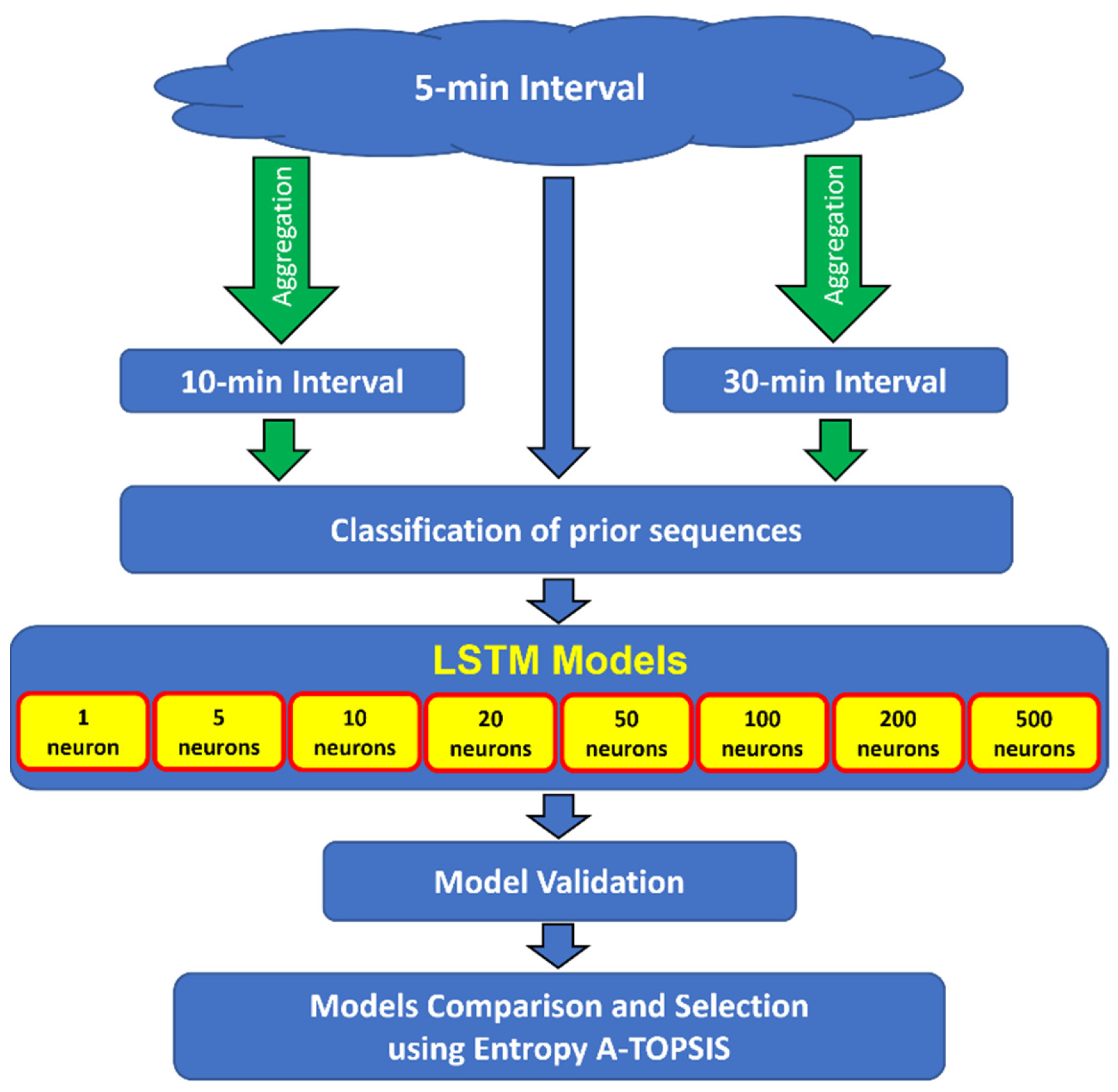
3.3. Forecasting Discharges Using Aggregated Time Intervals

With the most appropriate LSTM architecture, input, and output sequence dynamics realized from the previous section, we sought to ascertain the impact of data aggregation on predicting discharges. The 50-neuron LSTM architecture was used to forecast discharges for the next 1-h using the previous sequence of 1-h on the 10-min and 30-min aggregated dataset. The aggregated intervals were obtained by aggregating the original interval with frequencies of 10-min and 30-min. The results are compared with the original 5-min data and presented in Figure 6. Calculations of MAPE, RMSE, and R² of different intervals are shown in

Table 3. Comparison of differences between original and aggregated intervals.

Aggregation	MAPE	RMSE (×10−3)	R2
5-min Interval	0.118	0.996	0.674
10-min Interval	0.069	1.265	0.866
30-min Interval	0.072	3.835	0.859

.

As expected, the results show that the RMSE increases with increasing data aggregation intervals. Specifically, RMSE increases from 0.996 to 1.265 when the aggregation interval increases from 5-min to 10-min. However, this value increases by almost nine times when the aggregation interval changes from 10-min to 30-min. The predictions from the 5-min and 30-min interval data had a lower performance than the 10-min interval. This is reflected by a decreasing trend of MAPE (from 0.118 to 0.069) and an increasing trend of R² (0.674 to 0.866) from 5-min to 10-min intervals and corresponding opposite changes of these values when the aggregation interval increases from 10-min to 30-min. Even though the original (5-min interval) data have a very high temporal resolution, they do not contain more information about the pattern of the discharges than the aggregated data. We presume that the high-intensity data fluctuate a great deal and therefore have no general pattern for ML or deep learning algorithms to learn. The aggregated data lessen the impact of these fluctuations and present a more tractable pattern for ML and deep learning algorithms to learn. Comparatively, the 10-min data aggregations presented better results.

4. Discussion

The results in this study agree with a previous study by Tran et al. [70], where it was shown that a deep neural network with fewer hidden neurons could perform better than complex architecture in time-series prediction. Likewise, Thi Kieu Tran et al. [71] showed that a single hidden layer neural network (including ANN, RNN, and LSTM) had better performance compared to two or three hidden layers in forecasting temperature. Moreover, the study by Lee et al. [72] achieved better performance in forecasting rainfall when the number of independent variables, and the number of neurons in the hidden layer decreased from 11 to 5 and from 4 to 2, respectively. This could be explained by an excessively complex neural network architecture (too many hidden layers and/or neurons in the hidden layer(s)) might lead to time-consuming, useless processes [73] and over-fitting [74]. In contrast, an excessively simple neural network obviously cannot learn much useful information from input patterns and results in increased errors and under-fitting [70,75].

The study by Ke and Liu [73] proposed a formula for calculating optimum neurons in the hidden layer of the neural network model, and several rules-of-thumb criteria for choosing appropriate hidden layer neurons were introduced in the research of Gaurang et al. [75]. In general, these studies discover the relationship between the number of hidden neurons and the number of input/outputs. Furthermore, they concluded that these rules were not always valid for all cases. The results in this study strengthen these conclusions. In particular, when input sequences changed (24–36 steps in Table 1 or 12–24 steps in Table 2), the optimal neurons in the hidden layer remained at 50. This could be explained by the noise degree in the sample dataset [73]. If the degree of the noise of the input sample does not change significantly, increasing input sequence length cannot affect hidden neurons remarkably. Therefore, preprocessing data to decrease noise or eliminate outliers should be considered before building ANN to improve prediction performance and accuracy.

Choosing optimal sampling intervals to improve modeling performance significantly depends on the kind of dataset and research purposes. For example, high sampling resolutions of 10-s to 1-min outperformed 5-min to 15-min resolution in quickly detecting small leakages in a water-use simulation [76]. On the other hand, in a water distribution network, Kirstein et al. [77] showed that sampling intervals below 30-min could not further improve model calibration accuracy and applicability. The above examples indicate that sampling intervals should be considered to improve discharge’s predicted performance in the sewer network. This study reveals that the 10-min aggregation data from the original 5-min interval can improve predicting performance in the study area.

An advantage of data aggregation is that it does not only help with clear pattern(s) recognition in the data, but it also reduces the cost of SCADA operation. Power consumption, transmission bandwidth, and storage space are reduced while significantly achieving better accuracy on future prediction of discharges. Saving energy, enhancing storage capability, and improving prediction accuracy are highly critical to networks, which use wireless sensors to monitor and transfer data. For example, the lifetime of a Wireless Sensor Network (WSN) was impressively improved from only a few days to 418 days by implementing data aggregation [78]. Data aggregation was proven to be a helpful technique in reducing power consumption and enhancing the lifetime of WSN [79,80]. Based on results in this study, utilizing the 10-min aggregated data, a potential cost saving of 50% could be realized if the frequency of the data acquisition system deployed by Regnbyge.no is increased from 5-min to 10-min. This study has shown that it is possible to achieve better performance on discharge prediction using low-frequency data, which better represents the inherent trend in the data. However, the study is not without limitations. The LSTM algorithms take much time to execute, as it takes a significant amount of time for the hyperparameters of the network to be optimized. Secondly, the LSTM architectures obtained in this study were based on only one discharge location in the sewer network and may therefore not be applicable to other locations with different discharge patterns.

5. Conclusions

This study explores the potential application of an LSTM model for forecasting discharges in a combined sewer pipe using the sequence-to-sequence technique. Different LSTM architectures were implemented and ranked using entropy A-TOPSIS. The results showed that an LSTM model with very few neurons in the hidden layer did not effectively predict discharges. Increasing neurons in the hidden layer can help the LSTM model learn the dataset’s characteristics effectively and produce reliable predictions. However, the LSTM model with excessive neurons in the hidden layer performed poorly. Using about 50 neurons in the hidden layer produced very good predictions. Various sequence input data have been investigated to forecast discharges. It was shown that using excessive data input can make the LSTM model operate in an unstable state, and the accuracy of forecasted values becomes unpredictable. Different prior and subsequent inputs affect the optimal number of neurons in the hidden layer, resulting in reduced model prediction performance. Equal input and output sequences present the best results in terms of discharge forecast accuracy.

This study also showed that increasing the signal receiving frequency can improve the accuracy of discharge prediction. However, using high-frequency data will reduce the forecasting accuracy in the LSTM model and consume more storage, transmission bandwidth, and energy resources. This study showed that using a 10-min interval as an input sequence for the LSTM model performed better than a 5-min or 30-min interval for this particular study. Managers of sewer systems should consider setting up reasonably low signal-receiving frequency to capture the inherent trends in discharge data without excessive fluctuations.

The optimal entropy A-TOPSIS inspired LSTM will be implemented in a real-time stormwater-control strategy in collaboration with the Ålesund Municipality as a part of a Smart Water Project. The implementation will be based on long-term flow data, which are currently being collected in the sewer network using a network of flow sensors.

References

1. Butler, D.; Digman, C.; Makropoulos, C.; Davies, J.W. Urban Drainage, 4th ed.; CRC Press, Taylor & Francis Group: Boca Raton, FL, USA, 2018. [Google Scholar]
2. Water, N. The Water Services in Norway; Vangsvegen 143: Hamar, Norway, 2014. [Google Scholar]
3. Petrie, B. A review of combined sewer overflows as a source of wastewater-derived emerging contaminants in the environment and their management. Environ. Sci. Pollut. Res. 2021, 28, 32095–32110. [Google Scholar] [CrossRef]
4. Hernes, R.R.; Gragne, A.S.; Abdalla, E.M.H.; Braskerud, B.C.; Alfredsen, K.; Muthanna, T.M. Assessing the effects of four SUDS scenarios on combined sewer overflows in Oslo, Norway: Evaluating the low-impact development module of the Mike Urban model. Hydrol. Res. 2020, 51, 1437–1454. [Google Scholar] [CrossRef]
5. Nilsen, V.; Lier, J.A.; Bjerkholt, J.T.; Lindholm, O.G. Analysing urban floods and combined sewer overflows in a changing climate. J. Water Clim. Chang. 2011, 2, 260–271. [Google Scholar] [CrossRef]
6. Sun, Y.; Zhu, F.; Chen, J.; Li, J. Risk Analysis for Reservoir Real-Time Optimal Operation Using the Scenario Tree-Based Stochastic Optimization Method. Water 2018, 10, 606. [Google Scholar] [CrossRef] [Green Version]
7. Report of the 17th Meeting (16–17 May 2019) to the International Committee for Weights and Measures; Consultative Committee for Mass and Related Quantities (CCM), Bureau International des Poids et Mesures: Sèvres, France, 2019; p. 29.
8. Alihosseini, M.; Thamsen, P.U. Analysis of sediment transport in sewer pipes using a coupled CFD-DEM model and experimental work. Urban Water J. 2019, 16, 259–268. [Google Scholar] [CrossRef]
9. Butler, D.; May, R.; Ackers, J. Self-Cleansing Sewer Design Based on Sediment Transport Principles. J. Hydraul. Eng. 2003, 129, 276–282. [Google Scholar] [CrossRef]
10. Fu, X.; Goddard, H.; Wang, X.; Hopton, M.E. Development of a scenario-based stormwater management planning support system for reducing combined sewer overflows (CSOs). J. Environ. Manag. 2019, 236, 571–580. [Google Scholar] [CrossRef]
11. Hanssen-Bauer, I.; Førland, E.J.; Haddeland, I.; Hisdal, H.; Lawrence, D.; Mayer, S.; Nesje, A.; Nilsen, J.E.Ø.; Sandven, S.; Sandø, A.B.; et al. Climate in Norway 2100—A knowledge base for climate adaptation. NCCS Rep. 2017, 1, 2017. [Google Scholar]
12. Wang, W.-C.; Chau, K.-W.; Cheng, C.-T.; Qiu, L. A comparison of performance of several artificial intelligence methods for forecasting monthly discharge time series. J. Hydrol. 2009, 374, 294–306. [Google Scholar] [CrossRef] [Green Version]
13. Zhang, D.; Erlend; Lindholm, G.; Ratnaweera, H. Enhancing Operation of a Sewage Pumping Station for Inter Catchment Wastewater Transfer by Using Deep Learning and Hydraulic Model. arXiv Prepr. 2018, 1811, 06367. [Google Scholar]
14. Zhang, D.; Martinez, N.; Lindholm, G.; Ratnaweera, H. Manage Sewer In-Line Storage Control Using Hydraulic Model and Recurrent Neural Network. Water Resour. Manag. 2018, 32, 2079–2098. [Google Scholar] [CrossRef]
15. Saleh, F.; Ducharne, A.; Flipo, N.; Oudin, L.; Ledoux, E. Impact of river bed morphology on discharge and water levels simulated by a 1D Saint–Venant hydraulic model at regional scale. J. Hydrol. 2013, 476, 169–177. [Google Scholar] [CrossRef]
16. Habert, J.; Ricci, S.; Le Pape, E.; Thual, O.; Piacentini, A.; Goutal, N.; Jonville, G.; Rochoux, M. Reduction of the uncertainties in the water level-discharge relation of a 1D hydraulic model in the context of operational flood forecasting. J. Hydrol. 2016, 532, 52–64. [Google Scholar] [CrossRef] [Green Version]
17. Wu, X.-L.; Xiang, X.-H.; Wang, C.-H.; Chen, X.; Xu, C.-Y.; Yu, Z. Coupled Hydraulic and Kalman Filter Model for Real-Time Correction of Flood Forecast in the Three Gorges Interzone of Yangtze River, China. J. Hydrol. Eng. 2013, 18, 1416–1425. [Google Scholar] [CrossRef]
18. Box, G.E.; Jenkins, G.M.; Reinsel, G.C.; Ljung, G.M. Time Series Analysis: Forecasting and Control; John Wiley & Sons: Hoboken, NJ, USA, 2015. [Google Scholar]
19. Valipour, M.; Banihabib, M.E.; Behbahani, S.M.R. Comparison of the ARMA, ARIMA, and the autoregressive artificial neural network models in forecasting the monthly inflow of Dez dam reservoir. J. Hydrol. 2013, 476, 433–441. [Google Scholar] [CrossRef]
20. Valipour, M. Number of required observation data for rainfall forecasting according to the climate conditions. Am. J. Sci. Res. 2012, 74, 79–86. [Google Scholar]
21. Uvo, C.B.; Graham, N.E. Seasonal runoff forecast for northern South America: A statistical model. Water Resour. Res. 1998, 34, 3515–3524. [Google Scholar] [CrossRef]
22. Rosenberg, E.A.; Wood, A.W.; Steinemann, A.C. Statistical applications of physically based hydrologic models to seasonal streamflow forecasts. Water Resour. Res. 2011, 47, W00h14. [Google Scholar] [CrossRef]
23. Apel, H.; Abdykerimova, Z.; Agalhanova, M.; Baimaganbetov, A.; Gavrilenko, N.; Gerlitz, L.; Kalashnikova, O.; Unger-Shayesteh, K.; Vorogushyn, S.; Gafurov, A. Statistical forecast of seasonal discharge in Central Asia using observational records: Development of a generic linear modelling tool for operational water resource management. Hydrol. Earth Syst. Sci. 2018, 22, 2225–2254. [Google Scholar] [CrossRef] [Green Version]
24. Lee, Y.-S.; Tong, L.-I. Forecasting time series using a methodology based on autoregressive integrated moving average and genetic programming. Knowl.-Based Syst. 2011, 24, 66–72. [Google Scholar] [CrossRef]
25. Li, J.; Zong, Q. The Forecasting of the Elevator Traffic Flow Time Series Based on ARIMA and GP. Adv. Mater. Res. 2012, 588–589, 1466–1471. [Google Scholar] [CrossRef]
26. Zhang, G.P. Time series forecasting using a hybrid ARIMA and neural network model. Neurocomputing 2003, 50, 159–175. [Google Scholar] [CrossRef]
27. Pai, P.-F.; Lin, C.-S. A hybrid ARIMA and support vector machines model in stock price forecasting. Omega 2005, 33, 497–505. [Google Scholar] [CrossRef]
28. Aladag, C.H.; Egrioglu, E.; Kadilar, C. Forecasting nonlinear time series with a hybrid methodology. Appl. Math. Lett. 2009, 22, 1467–1470. [Google Scholar] [CrossRef] [Green Version]
29. Vanrolleghem, P.A.; Kamradt, B.; Solvi, A.-M.; Muschalla, D. Making the best of two hydrological flow routing models: Nonlinear outflow-volume relationships and backwater effects model. In Proceedings of the 8th International Conference on Urban Drainage Modelling, Tokyo, Japan, 7–12 September 2009. [Google Scholar]
30. Qin, M.; Li, Z.; Du, Z. Red tide time series forecasting by combining ARIMA and deep belief network. Knowl.-Based Syst. 2017, 125, 39–52. [Google Scholar] [CrossRef]
31. Altwaijry, N.; Al-Turaiki, I. Arabic handwriting recognition system using convolutional neural network. Neural Comput. Appl. 2021, 33, 2249–2261. [Google Scholar] [CrossRef]
32. Kubanek, M.; Bobulski, J.; Kulawik, J. A Method of Speech Coding for Speech Recognition Using a Convolutional Neural Network. Symmetry 2019, 11, 1185. [Google Scholar] [CrossRef] [Green Version]
33. Araújo, R.d.A.; Nedjah, N.; Oliveira, A.L.I.; Meira, S.R.d.L. A deep increasing–decreasing-linear neural network for financial time series prediction. Neurocomputing 2019, 347, 59–81. [Google Scholar] [CrossRef]
34. Zhang, J.; Zhu, Y.; Zhang, X.; Ye, M.; Yang, J. Developing a Long Short-Term Memory (LSTM) based model for predicting water table depth in agricultural areas. J. Hydrol. 2018, 561, 918–929. [Google Scholar] [CrossRef]
35. Pavlyshenko, B.M. Machine-Learning Models for Sales Time Series Forecasting. Data 2019, 4, 15. [Google Scholar] [CrossRef] [Green Version]
36. Li, S.; Li, W.; Cook, C.; Zhu, C.; Gao, Y. Independently Recurrent Neural Network (IndRNN): Building A Longer and Deeper RNN. In Proceedings of the IEEE Conference on Computer Vision and Pattern Recognition, Salt Lake City, UT, USA, 18–23 June 2018; pp. 5457–5466. [Google Scholar]
37. Yue, B.; Fu, J.; Liang, J. Residual Recurrent Neural Networks for Learning Sequential Representations. Information 2018, 9, 56. [Google Scholar] [CrossRef] [Green Version]
38. Manaswi, N.K. RNN and LSTM, in Deep Learning with Applications Using Python: Chatbots and Face, Object, and Speech Recognition with TensorFlow and Keras; Apress: Berkeley, CA, USA, 2018; pp. 115–126. [Google Scholar]
39. Hochreiter, S.; Schmidhuber, J. Long Short-Term Memory. Neural Comput. 1997, 9, 1735–1780. [Google Scholar] [CrossRef]
40. Jenckel, M.; Bukhari, S.S.; Dengel, A. Training LSTM-RNN with Imperfect Transcription: Limitations and Outcomes. In Proceedings of the 4th International Workshop on Historical Document Imaging and Processing, Kyoto, Japan, 10–11 November 2017; Association for Computing Machinery: Kyoto, Japan, 2017; pp. 48–53. [Google Scholar]
41. Xu, D.; Cheng, W.; Zong, B.; Song, D.; Ni, J.; Yu, W.; Liu, Y.; Chen, H.; Zhang, X. Tensorized LSTM with Adaptive Shared Memory for Learning Trends in Multivariate Time Series. In Proceedings of the AAAI Conference on Artificial Intelligence, New York, NY, USA, 7–12 February 2020; Volume 34, pp. 1395–1402. [Google Scholar]
42. Cao, J.; Li, Z.; Li, J. Financial time series forecasting model based on CEEMDAN and LSTM. Phys. A Stat. Mech. Its Appl. 2019, 519, 127–139. [Google Scholar] [CrossRef]
43. Song, X.; Liu, Y.; Xue, L.; Wang, J.; Zhang, J.; Wang, J.; Jiang, L.; Cheng, Z. Time-series well performance prediction based on Long Short-Term Memory (LSTM) neural network model. J. Pet. Sci. Eng. 2020, 186, 106682. [Google Scholar] [CrossRef]
44. Kuhn, M.; Johnson, K. An Introduction to Feature Selection, in Applied Predictive Modeling; Springer: New York, NY, USA, 2013; pp. 487–519. [Google Scholar]
45. Norway, S. Statistics Norway. 2020. Available online: https://www.ssb.no/kommunefakta/ (accessed on 20 April 2020).
46. CLIMATE-DATA.ORG. Ålesund Climate: Average Temperature, Weather by Month, Ålesund Water Temperature—Climate-Data.org. 2021. Available online: https://en.climate-data.org/europe/norway/m%C3%B8re-og-romsdal/alesund-9937/ (accessed on 20 April 2020).
47. Zhang, D.; Lindholm, G.; Ratnaweera, H. Use long short-term memory to enhance Internet of Things for combined sewer overflow monitoring. J. Hydrol. 2018, 556, 409–418. [Google Scholar] [CrossRef]
48. Yu, Y.; Si, X.; Hu, C.; Zhang, J. A Review of Recurrent Neural Networks: LSTM Cells and Network Architectures. Neural Comput. 2019, 31, 1235–1270. [Google Scholar] [CrossRef] [PubMed]
49. Greff, K.; Srivastava, R.K.; Koutník, J.; Steunebrink, B.R.; Schmidhuber, J. LSTM: A Search Space Odyssey. IEEE Trans. Neural Netw. Learn. Syst. 2017, 28, 2222–2232. [Google Scholar] [CrossRef] [Green Version]
50. Salman, A.G.; Heryadi, Y.; Abdurahman, E.; Suparta, W. Single Layer & Multi-layer Long Short-Term Memory (LSTM) Model with Intermediate Variables for Weather Forecasting. Procedia Comput. Sci. 2018, 135, 89–98. [Google Scholar]
51. Li, Y.; Cao, H. Prediction for Tourism Flow based on LSTM Neural Network. Procedia Comput. Sci. 2018, 129, 277–283. [Google Scholar] [CrossRef]
52. Tien Bui, D.; Pradhan, B.; Lofman, O.; Revhaug, I.; Dick, O.B. Landslide susceptibility assessment in the Hoa Binh province of Vietnam: A comparison of the Levenberg–Marquardt and Bayesian regularized neural networks. Geomorphology 2012, 171–172, 12–29. [Google Scholar] [CrossRef]
53. Krohling, R.A.; Pacheco, A.G.C. A-TOPSIS—An Approach Based on TOPSIS for Ranking Evolutionary Algorithms. Procedia Comput. Sci. 2015, 55, 308–317. [Google Scholar] [CrossRef] [Green Version]
54. Pacheco, A.G.C.; Krohling, R.A. Ranking of Classification Algorithms in Terms of Mean–Standard Deviation Using A-TOPSIS. Ann. Data Sci. 2018, 5, 93–110. [Google Scholar] [CrossRef] [Green Version]
55. Vazquezl, M.Y.L.; Peñafiel, L.A.B.; Muñoz, S.X.S.; Martinez, M.A.Q. A Framework for Selecting Machine Learning Models Using TOPSIS. In International Conference on Applied Human Factors and Ergonomics; Springer: Cham, Switzerland, 2021; pp. 119–126. [Google Scholar]
56. Jingwen, H. Combining entropy weight and TOPSIS method For information system selection. In Proceedings of the 2008 IEEE International Conference on Automation and Logistics, Qingdao, China, 1–3 September 2008. [Google Scholar]
57. Deng, H.; Yeh, C.-H.; Willis, R.J. Inter-company comparison using modified TOPSIS with objective weights. Comput. Oper. Res. 2000, 27, 963–973. [Google Scholar] [CrossRef]
58. Scikit Learn. Available online: https://scikit-learn.org/stable/modules/model_evaluation.html#mean-absolute-percentage-error (accessed on 15 May 2021).
59. Lee, T.; Shin, J.-Y.; Kim, J.-S.; Singh, V.P. Stochastic simulation on reproducing long-term memory of hydroclimatological variables using deep learning model. J. Hydrol. 2020, 582, 124540. [Google Scholar] [CrossRef]
60. Gauch, M.; Kratzert, F.; Klotz, D.; Nearing, G.; Lin, J.; Hochreiter, S. Rainfall–runoff prediction at multiple timescales with a single Long Short-Term Memory network. Hydrol. Earth Syst. Sci. 2021, 25, 2045–2062. [Google Scholar] [CrossRef]
61. Wikipedia. Keras. 2021. Available online: https://en.wikipedia.org/wiki/Keras (accessed on 12 May 2021).
62. Li, X.-M.; Ma, Y.; Leng, Z.-H.; Zhang, J.; Lu, X.-X. High-Accuracy Remote Sensing Water Depth Retrieval for Coral Islands and Reefs Based on LSTM Neural Network. J. Coast. Res. 2020, 102, 21–32. [Google Scholar] [CrossRef]
63. Chen, X.; Feng, F.; Wu, J.; Liu, W. Anomaly detection for drinking water quality via deep biLSTM ensemble. In Proceedings of the Genetic and Evolutionary Computation Conference Companion, Kyoto, Japan, 15–19 July 2018; Association for Computing Machinery: Kyoto, Japan, 2018; pp. 3–4. [Google Scholar]
64. Muharemi, F.; Logofătu, D.; Leon, F. Machine learning approaches for anomaly detection of water quality on a real-world data set. J. Inform. Telecommun. 2019, 3, 294–307. [Google Scholar] [CrossRef] [Green Version]
65. Chimmula, V.K.R.; Zhang, L. Time series forecasting of COVID-19 transmission in Canada using LSTM networks. Chaos Solitons Fractals 2020, 135, 109864. [Google Scholar] [CrossRef] [PubMed]
66. Li, W.; Liu, Z. A method of SVM with Normalization in Intrusion Detection. Procedia Environ. Sci. 2011, 11, 256–262. [Google Scholar] [CrossRef] [Green Version]
67. Troiano, L.; Villa, E.M.; Loia, V. Replicating a Trading Strategy by Means of LSTM for Financial Industry Applications. IEEE Trans. Ind. Inform. 2018, 14, 3226–3234. [Google Scholar] [CrossRef]
68. Salas, F.R.; Somos-Valenzuela, M.A.; Dugger, A.; Maidment, D.R.; Gochis, D.J.; David, C.H.; Yu, W.; Ding, D.; Clark, E.P.; Noman, N. Towards Real-Time Continental Scale Streamflow Simulation in Continuous and Discrete Space. JAWRA J. Am. Water Resour. Assoc. 2018, 54, 7–27. [Google Scholar] [CrossRef]
69. Brian Cosgrove, C.K. The National Water Model. Available online: https://water.noaa.gov/about/nwm (accessed on 8 June 2021).
70. Tran, T.T.; Lee, T.; Kim, J.-S. Increasing Neurons or Deepening Layers in Forecasting Maximum Temperature Time Series? Atmosphere 2020, 11, 1072. [Google Scholar] [CrossRef]
71. Thi Kieu Tran, T.; Lee, T.; Shin, J.-Y.; Kim, J.-S.; Kamruzzaman, M. Deep Learning-Based Maximum Temperature Forecasting Assisted with Meta-Learning for Hyperparameter Optimization. Atmosphere 2020, 11, 487. [Google Scholar] [CrossRef]
72. Lee, J.; Kim, C.-G.; Lee, J.E.; Kim, N.W.; Kim, H. Application of Artificial Neural Networks to Rainfall Forecasting in the Geum River Basin, Korea. Water 2018, 10, 1448. [Google Scholar] [CrossRef] [Green Version]
73. Ke, J.; Liu, X. Empirical Analysis of Optimal Hidden Neurons in Neural Network Modeling for Stock Prediction. In Proceedings of the 2008 IEEE Pacific-Asia Workshop on Computational Intelligence and Industrial Application, Wuhan, China, 19–20 December 2008. [Google Scholar]
74. Alam, S.; Kaushik, S.C.; Garg, S.N. Assessment of diffuse solar energy under general sky condition using artificial neural network. Appl. Energy 2009, 86, 554–564. [Google Scholar] [CrossRef]
75. Gaurang, P.; Ganatra, A.; Kosta, Y.; Panchal, D. Behaviour Analysis of Multilayer Perceptronswith Multiple Hidden Neurons and Hidden Layers. Int. J. Comput. Theory Eng. 2011, 3, 332–337. [Google Scholar]
76. Cominola, A.; Giuliani, M.; Castelletti, A.; Rosenberg, D.E.; Abdallah, A.M. Implications of data sampling resolution on water use simulation, end-use disaggregation, and demand management. Environ. Model. Softw. 2018, 102, 199–212. [Google Scholar] [CrossRef] [Green Version]
77. Kirstein, J.K.; Høgh, K.; Rygaard, M.; Borup, M. A case study on the effect of smart meter sampling intervals and gap-filling approaches on water distribution network simulations. J. Hydroinform. 2020, 23, 66–75. [Google Scholar] [CrossRef]
78. Croce, S.; Marcelloni, F.; Vecchio, M. Reducing Power Consumption in Wireless Sensor Networks Using a Novel Approach to Data Aggregation. Comput. J. 2007, 51, 227–239. [Google Scholar] [CrossRef]
79. Al-Karaki, J.N.; Ul-Mustafa, R.; Kamal, A.E. Data aggregation in wireless sensor networks—Exact and approximate algorithms. In Proceedings of the 2004 Workshop on High Performance Switching and Routing 2004, HPSR, Phoenix, AZ, USA, 19–21 April 2004. [Google Scholar]
80. Lazzerini, B.; Marcelloni, F.; Vecchio, M.; Croce, S.; Monaldi, E. A Fuzzy Approach to Data Aggregation to Reduce Power Consumption in Wireless Sensor Networks. In Proceedings of the NAFIPS 2006—2006 Annual Meeting of the North American Fuzzy Information Processing Society, Montreal, QC, Canada, 3–6 June 2006. [Google Scholar]
Figure 1. The overview of sample discharge and drainage network in the study area.
Water 14 00300 g001
Figure 2. Schematic of (a) RNN and (b) original LSTM architectures.
Water 14 00300 g002
Figure 3. Entropy A-TOPSIS ranking algorithm overview.
Water 14 00300 g003
Figure 4. The flowchart for data processing.
Water 14 00300 g004
Figure 5. Data distribution for training, validating, and testing the LSTM models.
Water 14 00300 g005
Figure 6. Forecast using (a) 5-min, (b) 10-min, and (c) 30-min intervals.
Water 14 00300 g006