Mitigation of Hydroelastic Responses in a Very Large Floating Structure by a Connected Vertical Porous Flexible Barrier

Abstract

The hydroelastic response of an elastic thin plate combined with a vertical porous flexible plate floating on a single- or a two-layer fluid is analyzed in the two-dimensional Cartesian coordinate system. The vertical and the horizontal plates are placed in an inverted-L shape and rigidly connected together. The problem is studied with the aid of the method of matched eigenfunction expansions within the framework of linear potential flow theory. The fluid is assumed to be inviscid and incompressible, and the motion is assumed to be irrotational. Time–harmonic incident waves of the traveling mode with a given angular frequency are considered. Then, the least-squares approximation method and the inner product are used to obtain the expansion coefficients of the velocity potentials. Graphical results show the interaction between the water waves and the structure. The effects of several physical parameters, including the length and the complex porous-effect parameter of the vertical plate, on the wave reflection and transmission are discussed. The results show that a vertical plate can effectively eliminate the hydroelastic response of the very large floating structure. The longer a vertical plate is, the more waves are reflected by the vertical plate. With the increase in the porous-effect parameter, the deflection of vertical plate decreases. Besides the effects of the flexural rigidity, the lateral stress, the mooring line angle, the fluid density ratio, and the position of interface on the wave reflection and transmission are discussed. Numerical results show the significant mitigation effect due to the presence of the additional vertical plate.

1. Introduction

Very large floating structures (VLFSs) have broad research prospects in the utilization of ocean space to deal with insufficient land. VLFSs can modularly be constructed for airports, storage facility, military base, etc. Thus, a VLFS is potentially able to alleviate the land scarcity caused by urban development. The large floating ice sheets and floes also play a similar role to build polar research bases and ice airports. According to the arguments from [1,2,3,4], VLFS have following advantages: long design life, low environmental impact, and ease of expansion and mobility. Due to the characteristics that a VLFS can follow the motion of a wave, which may cause structural fatigue and failure, it is necessary to install additional structures for suppressing the response of VLFS.

According to [5], excessive deformation of the VLFS would disrupt its feasibility as a floating runway or a floating storage facility. Moreover, it is necessary to eliminate low-frequency vibration of residential VLFS to ensure the comfort of residence. In order to suppress the hydroelastic responses of a VLFS, several methods have been introduced by Wang et al. [5] such as different kinds of breakwaters and the submerged plate anti-motion devices. A simple and effective anti-motion device is a submerged vertical plate attached with a VLFS, and it has been widely studied to suppress the hydroelastic response of a VLFS. Takagi et al. [6] concluded that, when a box-shaped body is attached to an edge of a VLFS, it reduces not only the deformation but also the shearing force and the moment of the platform, also attaining a good anti-motion performance. Masanobu et al. [7] proposed the additional wall with slits and the inverted-L type structures to mitigate the hydroelastic response of the VLFSs. They found that the drift force and the vertical displacement can be suppressed by providing slits for the anti-motion device. A composite grid method is adopted by Lee et al. [8] to solve the hydrodynamic forces and the nonlinear behaviors of fluid motion around a submerged plate. The added mass and damping forces on a VLFS were increased due to the generated vortex by the submerged plate, hence the structural responses were decreased. Taking a circle plate, for example, Pham et al. [9] utilized the modal expansion method to analyze the hydroelastic response of a pontoon-type circular VLFS attaching a horizontal submerged annular plate. The hydroelastic response reduction efficiency of VLFS edged with dual inclined plates has been investigated by Cheng et al. [10] with the aid of the method of matched eigenfunction expansions (MMEE). The finite element–boundary element method is utilized in research of a Wave Energy Converter (WEC)-type attachment to reduce hydroelastic responses of the VLFS [11,12]. Feng et al. [13] investigated the hydroelastic responses of a submerged horizontal solid/porous plate connected to a VLFS. On basis of understanding the above research, we think it is worth studying to suppress the deformation of VLFS with an additional vertical flexible plate.

Due to the feature that the horizontal size of the VLFS is much larger than its thickness, the flexible deformation of VLFS should be fully considered, while the rigid-body motion can be neglected. The pontoon-type VLFS was regarded by Ohmatsu [14] as a huge flat plate floating over the surface of water. Squire [15] claimed that there is a conspicuous overlap between the research in VLFS and in ice sheets. Thus, the VLFS model is also available for the analysis of floating ice sheets by using parameters of the ice. The MMEE was utilized to study the interaction between surface waves and an ice sheet by Fox and Squire [16], in which the unknowns coefficients were obtained by the error function method. The key of MMEE, which is often used in hydroelastic problems, is to obtain the expansion coefficients. Another method to find the expansion coefficients is to derive an orthogonal inner product in the plate-covered region [17]. Furthermore, when the physical model has an open region, the orthogonality of the eigenfunctions in the open region can be utilized. Xu and Lu [18] directly dealt with the problem by using the inner product which involves the orthogonal eigenfunctions in open region. In a two-layer fluid model, the dispersion relation have two pairs of real roots which represent the surface and interfacial traveling wave modes, and the interaction between surface waves and interface waves is important. Xu and Lu [19] proposed a new inner product which utilizes the orthogonality of the eigenfunctions in the open region on a two-layer fluid. Meng and Lu [20] investigated the hydroelastic response of an elastic plate with lateral internal forces in a small amplitude waves on a three-layer fluid.

The porous structures which can dissipate a part of wave energy are studied to suppress the waves. Yu and Chwang [21] suggested a newly derived boundary condition with a complex porous-effect parameter for the porous breakwaters in a semi-circular harbor. Yip et al. [22] investigated the trapping of surface waves by submerged vertical porous and flexible barriers near the end of a semi-infinitely long channel of finite depth. The full reflection always occurs when the distance between the channel end-wall and the barrier is an integer multiple of half-wavelength. Kumar and Sahoo [23] studied the performance of a flexible porous plate breakwater in a two-layer fluid via the least-squares approximation method which is widely used in research of vertical barrier. The highest wave reflection and the lowest wave transmission amplitude in the surface and interface modes can be observed for the case which has zero porosity. The wave reflection and transmission in a two-layer fluid was found to be strongly dependent on the location of interface and the fluid density ratio. Mandal et al. [24] studied oblique wave scattering by multiple porous, flexible barriers in a two-layer fluid, and the condition for the Bragg resonance was derived in the case of multiple barriers. Singla et al. [25] analyzed the effectiveness of vertical solid permeable barriers located at a finite distance from a VLFS. The porosity of the structure can reduce 15–20% of the wave energy. However, the vertical flexible porous plate to mitigate the response of VLFS has not been considered in previous studies. Thus, a porous structure is also included in our research because it can dissipate the wave energy.

In the present paper, we investigate the hydroelastic responses of a semi-infinite floating plate combined with a vertical porous flexible plate under the wave action on a single-layer or a two-layer fluid of finite depth with the aid of the MMEE. The floating plate is much larger than the vertical plate. We neglect the rigid body motion of a VLFS. We assume that there is no gap between the horizonal elastic plate and the surface of water. The pressure from the elastic plate is included in the boundary conditions. Our focus is on how the vertical plates affects the hydroelastic response of VLFS. The inner product and the least square approximation are used to obtain a set of simultaneous equations for different boundary conditions, and the edge conditions are included as a part of the equation system. The conservation of energy is used to validate method of solution. In Section 2, we study the interaction between waves with semi-infinite or finite plates on a single-layer fluid. In Section 3, we extend the method to the case of a two-layer fluid. Numerical calculations for the analytical expressions and graphical results are performed in Section 4. Finally, conclusions are given in Section 5.

2. Hydroelastic Response on a Single-Layer Fluid

2.1. Wave Interaction with a Semi-Infinite Floating Plate

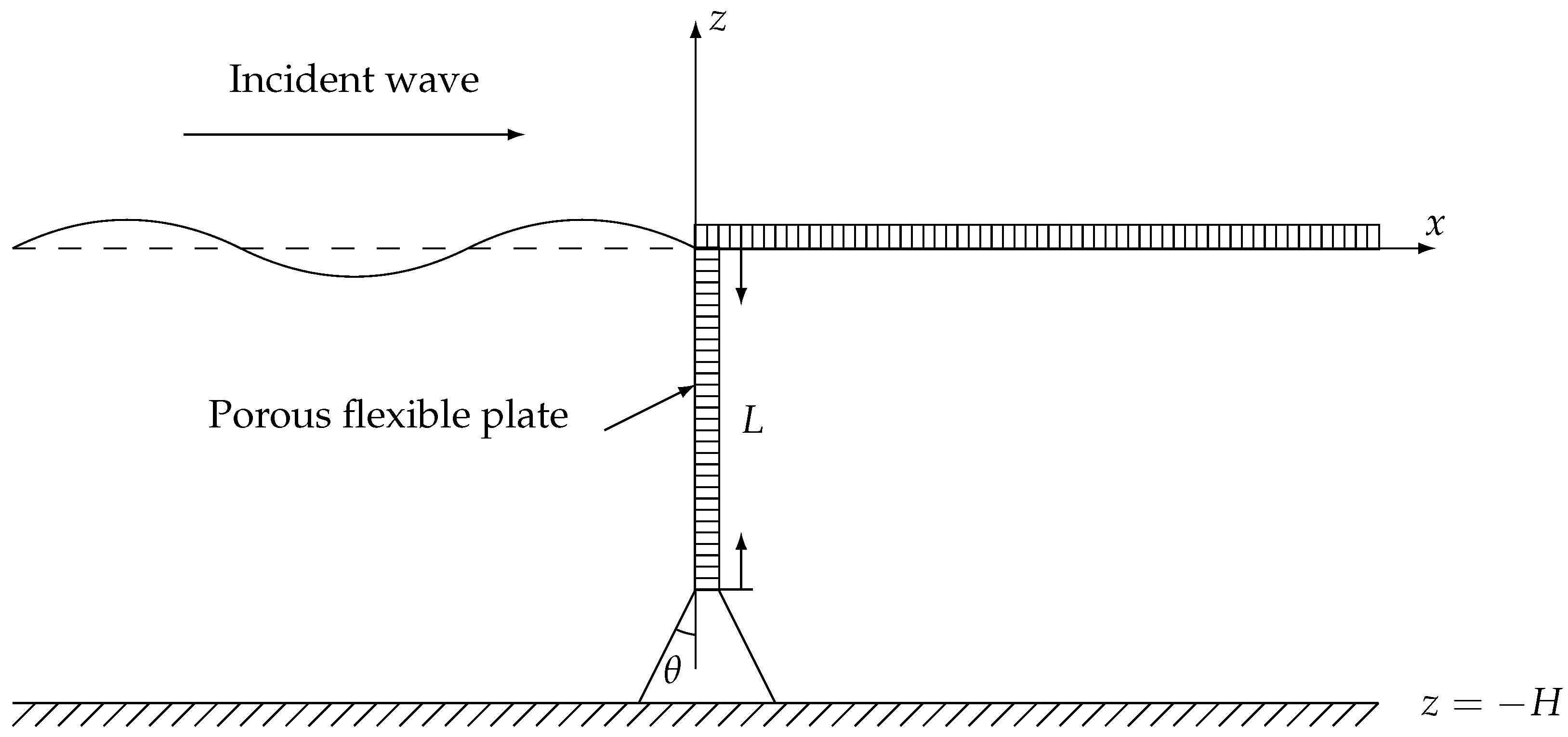
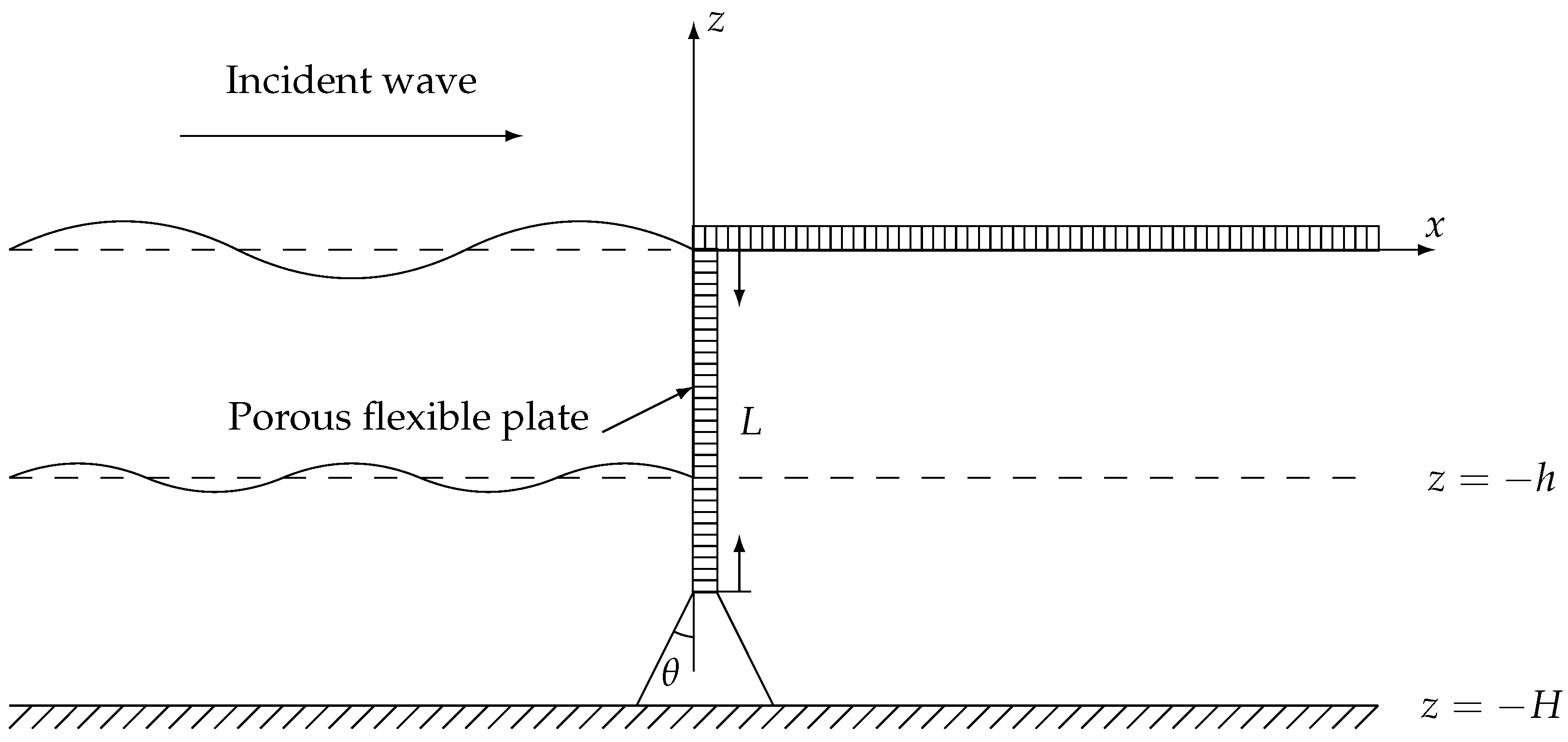
2.1.1. Mathematical Formulation

We consider the hydroelastic interaction between incident gravity waves and a semi-infinite floating elastic thin plate combined with a vertical finite porous flexible plate in a single-layer fluid bounded by a flat rigid seabead, as shown in Figure 1. A two-dimensional Cartesian coordinate system $oxz$ is chosen in such a way that the x-axis points the horizontally rightward and the z-axis point the vertically upward. The fluid with the constant density $\rho$ occupies the region $-H<z<0$ with $z=0$ being the undisturbed upper surface and $z=-H$ a flat bottom. The horizontal semi-infinite elastic plate which floats on the fluid with zero draft covers the region $0\le x<\infty$. The vertical elastic plate is fixed with the horizontal plate at $z=0$. The response of vertical plate is analyzed by assuming that the plate behaves as a one-dimensional beam. A clamped-mooring edge condition is used to describe the connection with the floating plate.

The fluid is assumed to be inviscid and incompressible and the fluid motion is considered irrotational. In the case of the simply time–harmonic motion with a frequency $\omega$, we can decompose the time factor and write the velocity potential $Re\left\{\varphi (x,z){\mathrm{e}}^{-\mathrm{i}\omega t}\right\}$ and the surface elevation $Re\left\{\zeta \left(x\right){\mathrm{e}}^{-\mathrm{i}\omega t}\right\}$, where $\varphi (x,z)$ is the spatial velocity potential, $\zeta \left(x\right)$ the spatial elevation on the surface and t the time variable. The whole flow domain is divided into two parts: the open water region $(-\infty <x<0)$ and the plate-covered region $(0<x<\infty )$, for which the corresponding spatial velocity potentials are denoted by ${\varphi }^{\mathrm{L}}(x,z)$ and ${\varphi }^{\mathrm{R}}(x,z)$, respectively. Thus, the governing equation is

$$\begin{array}{cc}\hfill & {\nabla }^2\varphi =0,(-\infty <x<\infty ,-H<z<0).\hfill \end{array}$$

(1)

The boundary condition at the flat bottom is

$$\begin{array}{cc}\hfill & \frac{\partial \varphi }{\partial z}=0,(-\infty <x<\infty ,z=-H).\hfill \end{array}$$

(2)

Within the framework of linear theory for small-amplitude waves, the combined kinematic and dynamic condition on the undisturbed surface $(z=0)$ for the open water region is given by

$$\begin{array}{cc}\hfill & -{\omega }^2{\varphi }^{\mathrm{L}}+g\frac{\partial {\varphi }^{\mathrm{L}}}{\partial z}=0,(-\infty <x<0,z=0),\hfill \end{array}$$

(3)

where g is the gravitational acceleration.

Under the assumption of no gap between the fluid and the horizontal plate, the combined kinematic and dynamic conditions for the plate-covered region on $z=0$ can be written as

$$\begin{array}{cccc}\hfill & -\rho {\omega }^2{\varphi }^{\mathrm{R}}+\left(\tilde{D}\frac{{\partial }^4}{\partial x^4}-{\tilde{M}}_{\mathrm{e}}{\omega }^2+\rho g\right)\frac{\partial {\varphi }^{\mathrm{R}}}{\partial z}=0,\hfill & \hfill & (0<x<\infty ,z=0),\hfill \end{array}$$

(4)

where ${\tilde{M}}_{\mathrm{e}}={\tilde{\rho }}_{\mathrm{e}}\tilde{d}$, $\tilde{D}=\tilde{E}{\tilde{d}}^3/\left[12(1-{\tilde{\nu }}^2)\right]$, and $\tilde{E}$, $\tilde{d}$, $\tilde{\nu }$, and ${\tilde{\rho }}_{\mathrm{e}}$ are the flexural rigidity, the effective Young modulus, the constant thickness, Poisson’s ratio, and the density of the horizontal plate, respectively.

As the vertical barrier is assumed to be a thin elastic plate of uniform mass subject to uniform rigidity, the equation of motion for the vertical plate acted upon by the fluid pressure is given by

$$\begin{array}{cccc}\hfill & D\frac{{\mathrm{d}}^4\xi }{\mathrm{d}{z}^4}+Q\frac{{\mathrm{d}}^2\xi }{\mathrm{d}{z}^2}-M_{\mathrm{e}}{\omega }^2\xi =\mathrm{i}\omega \rho ({\varphi }^{\mathrm{L}}-{\varphi }^{\mathrm{R}}),\hfill & \hfill & (x=0,-L<z<0),\hfill \end{array}$$

(5)

where $\xi =\xi \left(z\right)$ is the horizontal deflection of barrier, $M_{\mathrm{e}}={\rho }_{\mathrm{e}}d$, $D=E{d}^3/\left[12(1-{\nu }^2)\right]$, and E, d, $\nu$, L, and ${\rho }_{\mathrm{e}}$ are the flexural rigidity, the effective Young modulus, the constant thickness, Poisson’s ratio, the length, and the density of the vertical plate, respectively. Q is related to the lateral stress of the plate (with compression at $Q>0$ and stretch at $Q<0$).

With the aid of the Darcy law for describing the flow past a porous structure, the boundary condition on the vertical plate is given by

$$\begin{array}{cccc}\hfill & \frac{\partial \varphi }{\partial x}{|}_{x=0^{\pm }}=\mathrm{i}{k}_{0}G({\varphi }^{\mathrm{L}}-{\varphi }^{\mathrm{R}})-\mathrm{i}\omega \xi ,\hfill & \hfill & (x=0,-L<z<0),\hfill \end{array}$$

(6)

where

$$\begin{array}{c}\hfill G=\frac{\epsilon (f+\mathrm{i}S)}{k_{0}d(f^2+S^2)}\end{array}$$

(7)

is the complex porous-effect parameter defined by Yu and Chwang [21], $k_0$ the wavenumber of surface progressive wave mode, $\epsilon$ the porosity, f the linearized resistance coefficient, and S the inertial force coefficient. It is assumed that the porous plate has negligible storage capacity.

The matching relations for the continuities of pressure and velocity and along $x=0$ are given by

$$\begin{array}{cccc}\hfill & {\varphi }^{\mathrm{L}}{{|}_{x=0^{-}}={\varphi }^{\mathrm{R}}|}_{x=0^{+}},\hfill & \hfill & (-H\le z\le -L),\hfill \end{array}$$

(8)

$$\begin{array}{cccc}\hfill & \frac{\partial {\varphi }^{\mathrm{L}}}{\partial x}{|}_{x=0^{-}}=\frac{\partial {\varphi }^{\mathrm{R}}}{\partial x}{|}_{x=0^{+}},\hfill & \hfill & (-H\le z\le -L).\hfill \end{array}$$

(9)

The vanishing of deflection and slope at the clamped edge of the horizontal plate are given by

$$\begin{array}{cccc}\hfill & \frac{\partial {\varphi }^{\mathrm{R}}}{\partial z}{|}_{x=0^{+},z=0}=0,\hfill & \hfill & \frac{{\partial }^2{\varphi }^{\mathrm{R}}}{\partial x\partial z}{|}_{x=0^{+},z=0}=0.\hfill \end{array}$$

(10)

With the requirements of the clamped-mooring edge conditions in Mandal et al. [24], zero deflection and zero slope at the fixed edge require the conditions as follows:

$$\begin{array}{cccc}\hfill & \xi {|}_{z=0}=0,\hfill & \hfill & EI\frac{\partial \xi }{\partial z}{|}_{z=0}=0.\hfill \end{array}$$

(11)

At the edge near the mooring line, the bending moment is zero and the mooring tension relating to the elastic restoring force is added to the shearing force, which yields

$$\begin{array}{cccc}\hfill & \frac{{\partial }^2\xi }{\partial z^2}{|}_{z=-L}=0,\hfill & \hfill & EI\frac{{\partial }^3\xi }{\partial z^3}{|}_{z=-L}=2K_{\mathrm{m}}\xi {sin}^2\theta ,\hfill \end{array}$$

(12)

where $\theta$ is the mooring line angle and $K_{\mathrm{m}}$ the stiffness of the mooring line.

2.1.2. Method of Solution

In the framework of the MMEE, the vertical eigenfunction $V(k,z)$ for a single layer fluid reads

$$\begin{array}{cc}\hfill & V(k,z)=\frac{cosh\left[k\right(z+H\left)\right]}{cosh\left(kH\right)}.\hfill \end{array}$$

(13)

Thus the spatial velocity potentials can be written as

$$\begin{array}{cc}\hfill {\varphi }^{\mathrm{L}}(x,z)& =\left(I_0{\mathrm{e}}^{\mathrm{i}{k}_{0}x}+R_0{\mathrm{e}}^{-\mathrm{i}{k}_{0}x}\right)Z_0+\sum _{i=1}^{\infty }{R}_i{\mathrm{e}}^{k_{i}x}{Z}_i,\hfill \\ \hfill & =(I_0{\mathrm{e}}^{\mathrm{i}{k}_{0}x}+R_0{\mathrm{e}}^{-\mathrm{i}{k}_{0}x})Z_0+\sum _i{R}_i{\mathrm{e}}^{k_{i}x}{Z}_i,\hfill & \hfill & (x<0)\hfill \end{array}$$

(14)

$$\begin{array}{cc}\hfill {\varphi }^{\mathrm{R}}(x,z)& =T_0{\mathrm{e}}^{\mathrm{i}{\tilde{k}}_{0}x}\widetilde{Z_0}+\sum _{j=\mathrm{I}}^{\mathrm{II}}{T}_j{\mathrm{e}}^{-{\tilde{k}}_{j}x}\widetilde{Z_j}+\sum _{j=1}^{\infty }{T}_j{\mathrm{e}}^{-{\tilde{k}}_{j}x}\widetilde{Z_j},\hfill \\ \hfill & =T_0{\mathrm{e}}^{\mathrm{i}{k}_{0}x}\widetilde{Z_0}+\sum _j{T}_j{\mathrm{e}}^{-{\tilde{k}}_{j}x}\widetilde{Z_j},\hfill & \hfill & (x>0),\hfill \end{array}$$

(15)

where

$$\begin{array}{cc}\hfill & I_0=-\mathrm{i}\omega {\zeta }_0{\left[\frac{\partial V(k_0,0)}{\partial z}\right]}^{-1},\hfill \end{array}$$

(16)

$$\begin{array}{cc}\hfill & \{Z_0,Z_i,\widetilde{Z_0},\widetilde{Z_j}\}=\{V(k_0,z),V(\mathrm{i}{k}_i,z),V({\tilde{k}}_0,z),V(\mathrm{i}{\tilde{k}}_j,z)\},\hfill \end{array}$$

(17)

${\zeta }_0$ is the amplitudes of surface incident wave; the reflection coefficients $R_0$ and $R_i$ and the transmission coefficients $T_0$ and $T_j$ are complex numbers to be determined, where $(i=1,2,3,\dots ;j=\mathrm{I},\mathrm{II},1,2,3,\dots )$. $Z_0,Z_i,\widetilde{Z_0}$, and $\widetilde{Z_j}$ the vertical eigenfunctions. The symbols ${\sum }_i$ and ${\sum }_j$ are hereinafter defined as the summation signs for $i=1,2,3,\dots$ and $j=\mathrm{I},\mathrm{II},1,2,3,\dots$, respectively. Let positive real numbers $k_0$ and ${\tilde{k}}_0$ be the wave numbers of progressive wave modes. The purely imaginary numbers $k_i$ and ${\tilde{k}}_j$$(i,j=1,2,\cdots )$ are the wave numbers of evanescent modes in the open water and the plate-covered regions, respectively. Furthermore, ${\tilde{k}}_{\mathrm{I}}$ and ${\tilde{k}}_{\mathrm{II}}$ correspond to two decaying progressive waves in the plate-covered regions. For a given frequency $\omega$, the wave numbers $k_0$, $k_i$, and ${\tilde{k}}_j$ in Equations (14) and (15) satisfy

$$\begin{array}{ccc}\hfill {\omega }^2=g{k}_{0}tanh\left(k_{0}H\right)=-g{k}_{i}tan\left(k_{i}H\right),& \hfill & \hfill (i=1,2,3,\dots )\end{array}$$

(18)

$$\begin{array}{cc}\hfill {\omega }^2& =\frac{(1+\Gamma {\tilde{k}}_0^4)g{\tilde{k}}_{0}tanh\left({\tilde{k}}_{0}H\right)}{1+\sigma {\tilde{k}}_{0}tanh\left({\tilde{k}}_{0}H\right)}\hfill \\ \hfill & =-\frac{(1+\Gamma {\tilde{k}}_j^4)g{\tilde{k}}_{j}tan\left({\tilde{k}}_{j}H\right)}{1-\sigma {\tilde{k}}_{j}tan\left({\tilde{k}}_{j}H\right)},\hfill & \hfill & (j=\mathrm{I},\mathrm{II},1,2,\cdots ),\hfill \end{array}$$

(19)

where $\Gamma =\tilde{D}/\rho g$ and $\sigma ={\tilde{M}}_{\mathrm{e}}/\rho$. Equations (18) and (19) are called the dispersion relations for the waves in the open water and the plate-covered regions, respectively.

By substituting the velocity potentials in Equations (14) and (15) into Equation (5), a general solution for the governing equation of the vertical plate is of the following form

$$\begin{array}{c}\hfill \xi \left(z\right)=W-a_0(I_0+R_0)Z_0-\sum _i{a}_i{R}_i{Z}_i+{\tilde{a}}_0{T}_0\widetilde{Z_0}+\sum _j{\tilde{a}}_j{T}_j\widetilde{Z_j},\end{array}$$

(20)

where

$$\begin{array}{cc}\hfill & W\left(z\right)=\sum _{n=1}^2[C_{n}cosh\left({\kappa }_{n}z\right)+S_{n}sinh\left({\kappa }_{n}z\right)],\hfill \end{array}$$

(21)

$$\begin{array}{c}\hfill {\kappa }_n=\sqrt{\frac{{(-1)}^n\sqrt{4D{M}_{\mathrm{e}}+Q^2}-Q}{2D}},\end{array}$$

(22)

$$\begin{array}{cc}\hfill & a_i=\frac{\mathrm{i}\rho \omega }{(k_i-{\kappa }_1^2)(k_i-{\kappa }_2^2)},\hfill \end{array}$$

(23)

$$\begin{array}{cc}\hfill & {\tilde{a}}_j=\frac{\mathrm{i}\rho \omega }{({\tilde{k}}_j-{\kappa }_1^2)({\tilde{k}}_j-{\kappa }_2^2)},\hfill \end{array}$$

(24)

with the unknown coefficients $C_n$ and $S_n$$(n=1,2)$ to be determined by the boundary conditions of the vertical plate from Equations (11) and (12).

After substituting of the spatial velocity potentials Equations (14) and (15) into the matching relations Equations (8) and (9), it yields:

$$\begin{array}{cccc}\hfill & k_0(I_0-R_0)Z_0-\mathrm{i}\sum _i{k}_i{R}_i{Z}_i-{\tilde{k}}_0{T}_0\widetilde{Z_0}-\mathrm{i}\sum _j{\tilde{k}}_j{T}_j\widetilde{Z_j}=0,\hfill & \hfill & (-H<z<0),\hfill \end{array}$$

(25)

$$\begin{array}{cccc}\hfill & (I_0+R_0)Z_0+\sum _i{R}_i{Z}_i-T_0\widetilde{Z_0}-\sum _j{T}_j\widetilde{Z_j}=0,\hfill & \hfill & (-H<z<-L).\hfill \end{array}$$

(26)

In order to deduce the linear algebraic equations for the unknown expansion coefficients, we employ the inner product of the vertical eigenfunctions for a single layer fluid, which was defined by Xu and Lu [18] as follows,

$$\begin{array}{ccc}\hfill P_{il}={\int }_{-H}^0{Z}_i·Z_l\mathrm{d}z,& \hfill & \hfill (i,l=0,1,2,\cdots ).\end{array}$$

(27)

One can easily validate that

$$\begin{array}{cc}\hfill P_{il}& =\left\{\begin{array}{ccc}0,\hfill & \hfill & (i\ne l),\hfill \\ =\frac{2kH+sinh\left(2kH\right)}{4k{cosh}^2\left(kH\right)},\hfill & \hfill & (i=l).\hfill \end{array}\right.\hfill \end{array}$$

(28)

Applying the inner product on both sides of Equation (25) with the vertical eigenfunction $Z_i\left(z\right)$ in the open water region, we have

$$\begin{array}{cccc}\hfill & k_0(I_0-R_0)P_{0l}={\tilde{k}}_0{T}_0{Q}_{0l}+\mathrm{i}\sum _j{\tilde{k}}_j{T}_j{Q}_{jl},\hfill & \hfill & (l=0),\hfill \end{array}$$

(29)

$$\begin{array}{cccc}\hfill & -k_l{R}_l{P}_{ll}={\tilde{k}}_0{T}_0{Q}_{0l}+\mathrm{i}\sum _j{\tilde{k}}_j{T}_j{Q}_{jl},\hfill & \hfill & (l=1,2,\cdots ),\hfill \end{array}$$

(30)

where

$$\begin{array}{ccc}\hfill Q_{jl}={\int }_{-H}^0{Z}_l·\widetilde{Z_j}\mathrm{d}z,& \hfill & \hfill (j=0,\mathrm{I},\mathrm{II},1,2,\cdots ).\end{array}$$

(31)

Substituting of the spatial velocity potentials Equations (14) and (15) into the boundary condition on the vertical porous barrier Equation (6), we obtain

$$\begin{array}{cc}\hfill & \omega W-(\omega a_0+G{k}_0)I_0{Z}_0-(\omega a_0+G{k}_0)R_0{Z}_0-\sum _i(\omega a_i+G{k}_0)R_i{Z}_i\hfill \\ & (\omega {\tilde{a}}_0+G{k}_0+{\tilde{k}}_0)T_j\widetilde{Z_j}+\sum _j(\omega {\tilde{a}}_j+G{k}_0+{\tilde{k}}_j)T_j\widetilde{Z_j}=0,(-L<z<0).\hfill \end{array}$$

(32)

Applying the least-squares method from [23], it is derived that

$$\begin{array}{cc}\hfill & {\int }_{-H}^{-L}{\left|H_1\left(z\right)\right|}^2\mathrm{d}z+{\int }_{-L}^0|H_2{\left(z\right)|}^2\mathrm{d}z=minimum.\hfill \end{array}$$

(33)

Minimizing the above integral in Equation (33) with respect to $R_i$, which are the unknowns in the open region, we obtain

$$\begin{array}{cc}\hfill & {\int }_{-H}^{-L}{H}_1\left(z\right)\frac{\partial H_1^{\ast }\left(z\right)}{\partial R_i}\mathrm{d}z+{\int }_{-L}^0{H}_2\left(z\right)\frac{\partial H_2^{\ast }\left(z\right)}{\partial R_i}\mathrm{d}z=0,\hfill \end{array}$$

(34)

where the superscript “$\ast$“ denotes the complex conjugate. We truncate the system such that the numbers of evanescent modes in the open water and plate-covered regions are N, and Equation (34) provides $N+2$ linear equations.

Substituting for the velocity potentials from Equations (14) and (15) to Equation (10), we obtain two other equations

$$\begin{array}{cc}\hfill & {\left[T_0\frac{\partial \widetilde{Z_0}}{\partial z}-\sum _j{T}_j\frac{\partial \widetilde{Z_j}}{\partial z}\right]}_{z=0}=0,\hfill \end{array}$$

(35)

$$\begin{array}{cc}\hfill & {\left[{\tilde{k}}_0{T}_0\frac{\partial \widetilde{Z_0}}{\partial z}-\mathrm{i}\sum _j{\tilde{k}}_j{T}_j\frac{\partial \widetilde{Z_j}}{\partial z}\right]}_{z=0}=0.\hfill \end{array}$$

(36)

Thus, we derive a system of $2N+8$ equations from Equations (11), (12), (29), (30), (34), and (35) for $2N+8$ unknown coefficient $R_i$, $T_j$, $C_n$, and $S_n$$(i=0,1,2,3,\dots ,N;$$j=0,\mathrm{I},\mathrm{II},1,2,3,N,\dots ;$$n=1,2)$. The unknowns in the velocity potentials can be obtained by solving numerically this closed system.

2.2. Wave Interaction with a Finite Elastic Plate

In real situations, VLFS can also be modeled as a finite elastic thin plate. In this section, we will investigate the interaction of water waves with a finite floating plate combined with an attached vertical plate. The length of horizontal elastic plate is $\tilde{L}$, and the horizontal elastic plate has no draft floats on the fluid and covers the region $(0\le x\le \tilde{L})$. The whole flow domain is divided into three parts: the left open water region $(-\infty <x<0)$, the plate-covered region $(0\le x\le \tilde{L})$, and the right open water region $(\tilde{L}<x<\infty )$. The corresponding spatial velocity potentials are denoted by ${\varphi }^{\mathrm{L}}(x,z)$, ${\varphi }^{\mathrm{M}}(x,z)$, and ${\varphi }^{\mathrm{R}}(x,z)$, respectively. The governing equation, linearized boundary conditions, and the matching relations for the continuities of pressure and velocity for this case are the same as those given in Section 2.1.

The matching relations for the continuities of pressure and velocity at $x=L$ are given by

$$\begin{array}{cc}\hfill & \frac{\partial {\varphi }^{\mathrm{M}}}{\partial x}{|}_{x=\tilde{L}}=\frac{\partial {\varphi }^{\mathrm{R}}}{\partial x}{|}_{x=\tilde{L}},\hfill \end{array}$$

(37)

$$\begin{array}{cc}\hfill & {\varphi }^{\mathrm{M}}{|}_{x=\tilde{L}}={\varphi }^{\mathrm{R}}{|}_{x=\tilde{L}}.\hfill \end{array}$$

(38)

The clamped-free edge conditions of the horizontal plate read

$$\begin{array}{cccc}\hfill & \frac{\partial {\varphi }^{\mathrm{M}}}{\partial z}{|}_{x=0,z=0}=0,\hfill & \hfill & \frac{{\partial }^2{\varphi }^{\mathrm{M}}}{\partial x\partial z}{|}_{x=0,z=0}=0,\hfill \end{array}$$

(39)

$$\begin{array}{cccc}\hfill & \frac{{\partial }^2{\varphi }^{\mathrm{M}}}{\partial x\partial z}{|}_{x=\tilde{L},z=0}=0,\hfill & \hfill & \frac{{\partial }^3{\varphi }^{\mathrm{M}}}{\partial x^2\partial z}{|}_{x=\tilde{L},z=0}=0.\hfill \end{array}$$

(40)

According to the method of eigenfunction expansion, the spatial velocity potentials ${\varphi }^{\mathrm{L}}(x,z)$, ${\varphi }^{\mathrm{M}}(x,z)$, and ${\varphi }^{\mathrm{R}}(x,z)$ can be written as

$$\begin{array}{cccc}\hfill & {\varphi }^{\mathrm{L}}(x,z)=\left(I_0{\mathrm{e}}^{\mathrm{i}{k}_{0}x}+R_0^{\mathrm{L}}{\mathrm{e}}^{-\mathrm{i}{k}_{0}x}\right)Z_0+\sum _i{R}_i^{\mathrm{L}}{\mathrm{e}}^{k_{i}x}{Z}_i,\hfill & \hfill & (-\infty <x<0),\hfill \end{array}$$

(41)

$$\begin{array}{cc}\hfill {\varphi }^{\mathrm{M}}(x,z)=& T_0^{\mathrm{M}}{\mathrm{e}}^{\mathrm{i}{\tilde{k}}_{0}x}\widetilde{Z_0}+\sum _j{T}_j^{\mathrm{M}}{\mathrm{e}}^{-{\tilde{k}}_{j}x}\widetilde{Z_j}\hfill \\ \hfill & +R_0^{\mathrm{M}}{\mathrm{e}}^{-\mathrm{i}{\tilde{k}}_0(x-\tilde{L})}\widetilde{Z_0}+\sum _j{R}_j^{\mathrm{M}}{\mathrm{e}}^{{\tilde{k}}_j(x-\tilde{L})}\widetilde{Z_j},\hfill & \hfill & (0\le x\le \tilde{L}),\hfill \end{array}$$

(42)

$$\begin{array}{cccc}\hfill & {\varphi }^{\mathrm{R}}(x,z)=T_0^{\mathrm{R}}{\mathrm{e}}^{\mathrm{i}{k}_0(x-\tilde{L})}{Z}_0+\sum _i{T}_i^{\mathrm{R}}{\mathrm{e}}^{-k_j(x-\tilde{L})}{Z}_i,\hfill & \hfill & (\tilde{L}<x<\infty ),\hfill \end{array}$$

(43)

where $R_i^{\mathrm{L}}$, $R_j^{\mathrm{M}}$ and $T_j^{\mathrm{M}}$, $T_j^{\mathrm{R}}$$(i=0,1,2,3,\dots ;j=0,\mathrm{I},\mathrm{II},1,2,3,\dots )$ are the reflection and transmission coefficients to be determined, respectively. The derivation and calculation for the unknown coefficients $R_i^{\mathrm{L}}$, $R_j^{\mathrm{M}}$ and $T_j^{\mathrm{M}}$, $T_j^{\mathrm{R}}$ can be found in Appendix A.

3. Wave Interaction on a Two-Layer Fluid

Compared with the case of a single-layer fluid, the two-layer fluid has an interface which divides the upper and lower layers at $z=-h$. The densities of the upper and lower fluids are denoted by ${\rho }_1$ and ${\rho }_2$, respectively. Next, we choose the case of the semi-infinite plate as an example, as shown in Figure 2. The matching relations of velocity and pressure at the interface ($-\infty <x<\infty ,z=-h_1$) are given by

$$\begin{array}{cc}\hfill & \frac{\partial \varphi }{\partial z}{|}_{z=-h^{+}}=\frac{\partial \varphi }{\partial z}{|}_{z=-h^{-}},\hfill \end{array}$$

(44)

$$\begin{array}{cc}\hfill & \gamma \left[K\varphi -\frac{\partial \varphi }{\partial z}\right]{|}_{z=-h^{+}}=\left[K\varphi -\frac{\partial \varphi }{\partial z}\right]{|}_{z=-h^{-}},\hfill \end{array}$$

(45)

where $\gamma ={\rho }_1/{\rho }_2$ and $K={\omega }^2/g$ with $0<\gamma <1$.

The dispersion relations in the open water and the plate-covered regions on the two-layer fluid are presented as follows.

$$\begin{array}{cc}\hfill & {\omega }^4-gk{\omega }^2[tanh\left(kh\right)+tanh\left(k{h}_2\right)]+[g^2{k}^2(1-\gamma )+\gamma {\omega }^4]tanh\left(kh\right)tanh\left(k{h}_2\right)=0,\hfill \end{array}$$

(46)

$$\begin{array}{cc}\hfill & {\omega }^4-\tilde{k}{\omega }^2\left\{g\left[tanh\left(\tilde{k}h\right)+tanh\left(\tilde{k}{h}_2\right)\right]+\frac{\tilde{D}{\tilde{k}}^4-{\omega }^2{\tilde{M}}_{\mathrm{e}}}{{\rho }_1}\left[tanh\left(\tilde{k}h\right)+\gamma tanh\left(\tilde{k}{h}_2\right)\right]\right\}\hfill \\ \hfill & +\left\{\left[g^2{\tilde{k}}^2(1-\gamma )+\gamma {\omega }^4\right]+g{\tilde{k}}^2(1-\gamma )\frac{\tilde{D}{\tilde{k}}^4-{\omega }^2{\tilde{M}}_{\mathrm{e}}}{{\rho }_1}\right\}tanh\left(\tilde{k}h\right)tanh\left(\tilde{k}{h}_2\right)=0.\hfill \end{array}$$

(47)

Here, $h_2=H-h$. Let positive real numbers $k_{0_1}$, $k_{0_2}$, ${\tilde{k}}_{0_1}$, and ${\tilde{k}}_{0_2}$ be the wave numbers of progressive wave modes. $k_i$ and ${\tilde{k}}_j$$(i=0_1,0_2,1,2,\cdots ;j=0_1,0_2,\mathrm{I},\mathrm{II},1,2,\cdots )$ have the same meanings as it in Section 2.

According to the method of eigenfunction expansion, ${\varphi }^{\mathrm{L}}(x,z)$ and ${\varphi }^{\mathrm{R}}(x,z)$ can be written as

$$\begin{array}{cc}\hfill {\varphi }^{\mathrm{L}}(x,z)=& \sum _{m=1}^2\left(I_{0_m}{\mathrm{e}}^{\mathrm{i}{k}_{0_m}x}+R_{0_m}{\mathrm{e}}^{-\mathrm{i}{k}_{0_m}x}\right)Z_{0_m}+\sum _i{R}_i{\mathrm{e}}^{k_{i}x}{Z}_i,\hfill \end{array}$$

(48)

$$\begin{array}{cc}\hfill {\varphi }^{\mathrm{R}}(x,z)& =\sum _{m=1}^2{T}_{0_m}{\mathrm{e}}^{\mathrm{i}{\tilde{k}}_{0_m}x}{\tilde{Z}}_{0_m}+\sum _j{T}_j{\mathrm{e}}^{-{\tilde{k}}_{j}x}\widetilde{Z_j},\hfill \end{array}$$

(49)

where

$$\begin{array}{cc}\hfill & I_{0_1}=-\mathrm{i}\omega {\zeta }_0{\left[\frac{\partial V(k_{0_1},0)}{\partial z}\right]}^{-1},\hfill \end{array}$$

(50)

$$\begin{array}{cc}\hfill & I_{0_2}=-\mathrm{i}\omega {\eta }_0{\left[\frac{\partial V(k_{0_2},-h)}{\partial z}\right]}^{-1},\hfill \end{array}$$

(51)

$$\begin{array}{cc}\hfill & \{Z_{0_1},Z_{0_2},Z_i,{\tilde{Z}}_{0_1},{\tilde{Z}}_{0_2},\widetilde{Z_j}\}\hfill \\ \hfill & =\{V(k_{0_1},z),V(k_{0_2},z),V(\mathrm{i}{k}_i,z),V({\tilde{k}}_{0_1},z),V({\tilde{k}}_{0_2},z),V(\mathrm{i}{\tilde{k}}_j,z)\}.\hfill \end{array}$$

(52)

The terms $R_{0_m}$, $R_i$ and $T_{0_m}$$T_j$$(i=1,2,\cdots ;j=\mathrm{I},\mathrm{II},1,2,\cdots )$ are, respectively, the reflection and transmission coefficients to be determined, whereas ${\zeta }_0$ and ${\eta }_0$ are the amplitudes of incident waves on the surface and interface, respectively. The vertical eigenfunction $V(k,z)$ in Equation (52) for a two-layer fluid is defined by Xu and Lu [19] as follows

$$\begin{array}{c}\hfill V(k,z)=\left\{\begin{array}{c}\frac{1}{2K\gamma coshkH}\{K(1+\gamma )coshk(H+z)\hfill \\ +(1-\gamma )[Kcoshk(h-h_2+z)\hfill \\ +k(sinhk(h-h_2+z)-sinhk(H+z))\left]\right\},\hfill & \hfill & (-h<z<0),\hfill \\ \frac{coshk(H+z)}{coshkH},\hfill & \hfill & (-H<z<-h).\hfill \end{array}\right.\end{array}$$

(53)

The inner product on the two-layer fluid is from [19]

$$\begin{array}{cccc}\hfill P_{il}=& {\int }_{-H}^{-h}{Z}_i·Z_l\mathrm{d}z+\gamma {\int }_{-h}^0{Z}_i·Z_l\mathrm{d}z,\hfill & \hfill & (i,l=0_1,0_2,1,2,\cdots ).\hfill \end{array}$$

(54)

The derivation and calculation for the unknown coefficients $R_i^{\mathrm{L}}$, $R_i^{\mathrm{M}}$ and $T_j^{\mathrm{M}}$, $T_j^{\mathrm{R}}$ can be found in Appendix B.

When a VLFS is modeled as a finite elastic thin plate, ${\varphi }^{\mathrm{L}}(x,z)$, ${\varphi }^{\mathrm{M}}(x,z)$ and ${\varphi }^{\mathrm{R}}(x,z)$, can be written as

$$\begin{array}{cccc}\hfill {\varphi }^{\mathrm{L}}(x,z)=& \sum _{m=1}^2\left(I_{0_m}{\mathrm{e}}^{\mathrm{i}{k}_{0_m}x}+R_{0_m}^{\mathrm{L}}{\mathrm{e}}^{-\mathrm{i}{k}_{0_m}x}\right)Z_{0_m}+\sum _i{R}_i^{\mathrm{L}}{\mathrm{e}}^{k_{i}x}{Z}_i,\hfill & \hfill & (-\infty <x<0),\hfill \end{array}$$

(55)

$$\begin{array}{cc}\hfill {\varphi }^{\mathrm{M}}(x,z)=& \sum _{m=1}^2{T}_{0_m}^{\mathrm{M}}{\mathrm{e}}^{\mathrm{i}{\tilde{k}}_{0_m}x}{\tilde{Z}}_{0_m}+\sum _j{T}_j^{\mathrm{M}}{\mathrm{e}}^{-{\tilde{k}}_{j}x}\widetilde{Z_j}\hfill \\ \hfill & +\sum _{m=1}^2{R}_{0_m}^{\mathrm{M}}{\mathrm{e}}^{-\mathrm{i}{\tilde{k}}_{0_m}(x-\tilde{L})}{\tilde{Z}}_{0_m}+\sum _j{R}_j^{\mathrm{M}}{\mathrm{e}}^{{\tilde{k}}_j(x-\tilde{L})}\widetilde{Z_j},\hfill & \hfill & (0\le x\le \tilde{L}),\hfill \end{array}$$

(56)

$$\begin{array}{cccc}\hfill & {\varphi }^{\mathrm{R}}(x,z)=\sum _{m=1}^2{T}_{0_m}^{\mathrm{R}}{\mathrm{e}}^{\mathrm{i}{k}_{0_m}(x-\tilde{L})}{Z}_{0_m}+\sum _i{T}_i^{\mathrm{R}}{\mathrm{e}}^{-k_j(x-\tilde{L})}{Z}_i,\hfill & \hfill & (\tilde{L}<x<\infty ).\hfill \end{array}$$

(57)

We can also use the least-squares method as Equations (A19) and (A22) in which $R_i$ is replaced with $R_i^{\mathrm{L}}$, for $m=1,2$

$$\begin{array}{cc}\hfill H_m\left(z\right)=& -\sum _{n=1}^2(\omega a_{0_n}+G{k}_{0_1})(I_{0_n}+R_{0_n}^{\mathrm{L}})Z_{0_n}-\sum _i(\omega a_i+G{k}_0)R_i^{\mathrm{L}}{Z}_i\hfill \\ \hfill & +\sum _{n=1}^2(\omega {\tilde{a}}_{0_n}+G{k}_{0_1}+{\tilde{k}}_{0_n})T_{0_n}^{\mathrm{M}}{\tilde{Z}}_{0_n}+\sum _j(\omega {\tilde{a}}_j+G{k}_0+{\tilde{k}}_j)T_j^{\mathrm{M}}\widetilde{Z_j}\hfill \\ \hfill & +\sum _{n=1}^2\left[(1+{\mathrm{e}}^{\mathrm{i}{\tilde{k}}_{0_n}\tilde{L}})\omega {\tilde{a}}_{0_n}+{\mathrm{e}}^{\mathrm{i}{\tilde{k}}_{0_n}\tilde{L}}G{k}_{0_1}-{\mathrm{e}}^{\mathrm{i}{\tilde{k}}_{0_n}\tilde{L}}{\tilde{k}}_{0_n}\right]R_{0_n}^M{\tilde{Z}}_{0_n}\hfill \\ \hfill & +\sum _j\left[(1+{\mathrm{e}}^{\mathrm{i}{\tilde{k}}_j\tilde{L}})\omega {\tilde{a}}_j+{\mathrm{e}}^{\mathrm{i}{\tilde{k}}_j\tilde{L}}G{k}_{0_1}-{\mathrm{e}}^{\mathrm{i}{\tilde{k}}_j\tilde{L}}{\tilde{k}}_j\right]R_j^M\widetilde{Z_j}+\omega W,\hfill \end{array}$$

(58)

$$\begin{array}{cc}\hfill H_3\left(z\right)=& \sum _{n=1}^2(I_{0_n}+R_{0_n}^{\mathrm{L}})Z_{0_n}+\sum _i{R}_i^{\mathrm{L}}{Z}_i-\sum _{n=1}^2{T}_{0_n}^{\mathrm{M}}{\tilde{Z}}_{0_n}-\sum _{j=0}^{\infty }{T}_j^{\mathrm{M}}\widetilde{Z_j}\hfill \\ \hfill & -\sum _{n=1}^2{\mathrm{e}}^{\mathrm{i}{\tilde{k}}_{0_n}L}{R}_{0_n}^{\mathrm{M}}\widetilde{Z_0}-\sum _j{\mathrm{e}}^{\mathrm{i}{\tilde{k}}_{j}L}{R}_j^{\mathrm{M}}\widetilde{Z_j}.\hfill \end{array}$$

(59)

4. Results and Discussion

4.1. Rate of Energy Flux

We take the case on the two-layer fluid as an example. For the sake of clarity, the total depth of the two-layer fluid H, the gravitational acceleration g and the density of the upper fluid ${\rho }_1$ are chosen as the characteristic quantities to non-dimensionalize relative quantities. The nondimensional variables and parameters are

$$\begin{array}{cc}\hfill & \widehat{x}=\frac{x}{H},\widehat{y}=\frac{y}{H},\widehat{z}=\frac{z}{H},\widehat{k}=kH,\widehat{\omega }=\omega \sqrt{\frac{H}{g}},{\widehat{\zeta }}_0=\frac{{\zeta }_0}{H},{\widehat{\eta }}_0=\frac{{\eta }_0}{H},\hfill \\ \hfill & \widehat{\tilde{d}}=\frac{\tilde{d}}{H},{\widehat{\tilde{\rho }}}_{\mathrm{e}}=\frac{{\tilde{\rho }}_{\mathrm{e}}}{\rho },\widehat{\tilde{D}}=\frac{\tilde{D}}{{\rho }_{1}g{H}^4},\widehat{d}=\frac{d}{H},{\widehat{\rho }}_{\mathrm{e}}=\frac{{\rho }_{\mathrm{e}}}{\rho },\widehat{D}=\frac{D}{{\rho }_{1}g{H}^4},\hfill \\ \hfill & \widehat{h}=\frac{h}{H},\widehat{L}=\frac{L}{H},\widehat{\tilde{L}}=\frac{\tilde{L}}{H},\widehat{\varphi }=\frac{\varphi }{H\sqrt{gH}},\widehat{Q}=\frac{Q}{{\rho }_{1}g{H}^2},\widehat{K_{\mathrm{m}}}=\frac{K_{\mathrm{m}}}{{\rho }_{1}gH}.\hfill \end{array}$$

(60)

The symbol “$\widehat{}$“ over the nondimensional variables and parameters will be dropped hereinafter for clarity. The parameters used for the computation are $\tilde{d}=d=0.01$, ${\tilde{\rho }}_{\mathrm{e}}={\rho }_{\mathrm{e}}=0.9$, $\tilde{D}=D=0.05$, $K_{\mathrm{m}}=0.01$, and $\theta ={45}^{\circ }$. We assume that the incident waves predominantly consisting of surface and interfacial modes have the same frequency $\omega$.

According to the kinematic boundary conditions, the amplitudes of surface and interfacial elevations, $A_{\mathrm{S}}\left(x\right)$ and $A_{\mathrm{I}}\left(x\right)$, can be given by

$$\begin{array}{cc}\hfill & A_{\mathrm{S}}\left(x\right)=\frac{1}{\omega }∥\frac{\partial \varphi (x,0)}{\partial z}∥,\hfill \end{array}$$

(61)

$$\begin{array}{cc}\hfill & A_{\mathrm{I}}\left(x\right)=\frac{1}{\omega }∥\frac{\partial \varphi (x,-h_1)}{\partial z}∥.\hfill \end{array}$$

(62)

The amplitudes of the bending moment $M\left(x\right)$ and the shear force $Q\left(x\right)$ on the horizontal plate can be given by

$$\begin{array}{cc}\hfill & M\left(x\right)=\frac{D}{\omega }\left|\left|\frac{\partial \varphi (x,0)}{\partial x^2\partial z}\right|\right|,\hfill \end{array}$$

(63)

$$\begin{array}{cc}\hfill & Q\left(x\right)=\frac{D}{\omega }\left|\left|\frac{\partial \varphi (x,0)}{\partial x^3\partial z}\right|\right|,\hfill \end{array}$$

(64)

The amplitudes of the bending moment $M\left(z\right)$ and the shear force $Q\left(z\right)$ on the vertical plate can be given by

$$\begin{array}{cc}\hfill & M\left(z\right)=D\left|\left|\frac{\partial }{\partial z^2}\xi \left(z\right)\right|\right|,\hfill \end{array}$$

(65)

$$\begin{array}{cc}\hfill & Q\left(z\right)=D\left|\left|\frac{\partial }{\partial z^3}\xi \left(z\right)\right|\right|.\hfill \end{array}$$

(66)

To validate the above-mentioned method of solution, numerical examples are presented here. The conservation of the energy for the two-layer fluid under consideration can be written as

$$\begin{array}{cc}\hfill & E^{\mathrm{O}}=E^{\mathrm{P}},\hfill \end{array}$$

(67)

where $E^{\mathrm{O}}$ and $E^{\mathrm{P}}$ are the rates of energy flux in the open water and plate-covered regions, respectively. $E^{\mathrm{O}}$ and $E^{\mathrm{P}}$ can be written as

$$\begin{array}{cc}\hfill E^{\{\mathrm{O},\mathrm{P}\}}=& {\int }_{-1}^{-h}\mathrm{Re}\left[\frac{\partial {\Phi }_2^{\{\mathrm{O},\mathrm{P}\}}}{\partial t}{\left(\frac{\partial {\Phi }_2^{\{\mathrm{O},\mathrm{P}\}}}{\partial x}\right)}^{\ast }+{\left(\frac{\partial {\Phi }_2^{\{\mathrm{O},\mathrm{P}\}}}{\partial t}\right)}^{\ast }\frac{\partial {\Phi }_2^{\{\mathrm{O},\mathrm{P}\}}}{\partial x}\right]\mathrm{d}z\hfill \\ \hfill & +\gamma {\int }_{-h}^{{\zeta }_0}\mathrm{Re}\left[\frac{\partial {\Phi }_1^{\{\mathrm{O},\mathrm{P}\}}}{\partial t}{\left(\frac{\partial {\Phi }_1^{\{\mathrm{O},\mathrm{P}\}}}{\partial x}\right)}^{\ast }+{\left(\frac{\partial {\Phi }_1^{\{\mathrm{O},\mathrm{P}\}}}{\partial t}\right)}^{\ast }\frac{\partial {\Phi }_1^{\{\mathrm{O},\mathrm{P}\}}}{\partial x}\right]\mathrm{d}z,\hfill \end{array}$$

(68)

where ${\Phi }_m(x,y,z,t)$ is the velocity potential for the upper $(m=1)$ and lower $(m=2)$ fluids, and the superscripts “O” and “P” denote the open water and plate-covered regions, respectively.

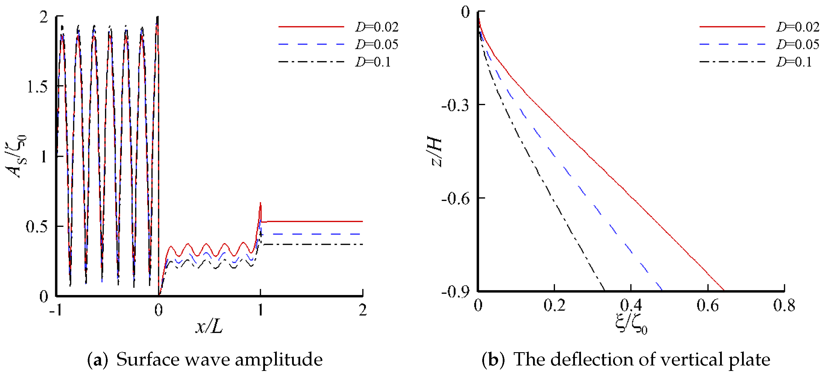
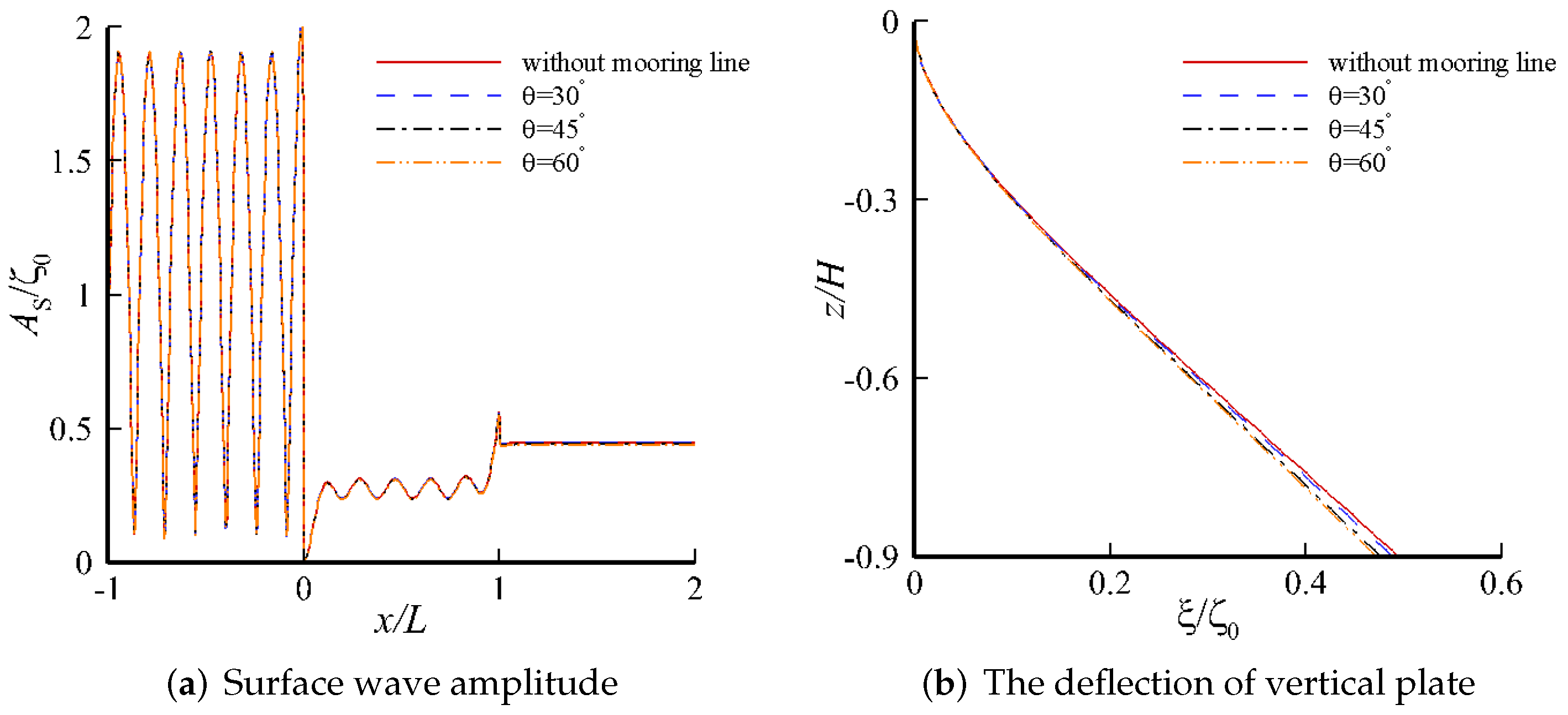
4.2. Response on a Single-Layer Fluid

In the present subsection, we consider the case of the semi-infinite plate model on a single-layer fluid, and set ${\zeta }_0=0.01$, $\omega =1.25$, $G=0$, $L=0.9$, and $N=15$ for calculations. The relative error of the energy is

$$\begin{array}{c}\hfill \frac{|E^{\mathrm{O}}-E^{\mathrm{P}}|}{min[E^{\mathrm{O}},E^{\mathrm{P}}]}\approx 1.964\%.\end{array}$$

(69)

Figure 3 illustrates the variation of the amplitudes of surface versus x and the horizontal deflection of the vertical plate versus z for various values of N, where N is the number of terms for the evanescent modes. It is obvious in Figure 3a that the changes of the curves are tiny enough to neglect. Figure 3b displays the horizontal deflection of the vertical plate which decreases slowly with the increment of N. It is depicted that the curves keep almost the same for $N\ge 15$ which reveals that the results of surface amplitudes converge quickly and the higher-order terms have a tiny contribution to the solution. Therefore we choose the parameter $N=15$ in the following cases.

Figure 4 reveals the effect of the length L of the vertical plate on the amplitudes of surface and the horizontal deflection of vertical plate. In this figure, the case without the vertical plate is also depicted for comparison reasons. It can be derived from Figure 4a that as L increases, the maximal amplitude of surface elevations increases in the left open water region while it decreases in the region behind the wall. The graph shows that the effect of the wall appears to increase reflection and decrease transmission. The changes of the curves between $L=0.7$ and $L=0.9$ is tiny enough to neglect. The reason for this phenomenon is that the energy of incident wave is mainly concentrated at the free surface and is reduced shapely with the decrement of the depth, and there is no need to extend the vertical plate to the bottom. From Figure 4b, it can be observed that the horizontal deflection and the rotating angle of vertical plate caused by fluid motion increase significantly with the increment of the length of the vertical plate.

Figure 5, Figure 6 and Figure 7 show the variations of the amplitudes of surface versus x and the horizontal deflection of the vertical plate versus z with different values of the frequency $\omega$ for finite and semi-infinite plates. It can be observed from Figure 5a that for a low frequency, i.e., $\omega =0.75$, the wave scattering due to the finite and semi-infinite plates is almost identical, except on the right open water region. It can be seen from the comparison among Figure 5a, Figure 6a, and Figure 7a that as $\omega$ increases, the amplitudes in the left open water region increase while an opposite trend is observed in the right open water region, indicating that the wave with the low $\omega$ has good penetration. From Figure 5b, Figure 6b, and Figure 7b, it can be observed that the horizontal deflection of vertical plate decreases with the increment of $\omega$. In summary, higher-frequency waves are more effectively suppressed by structures and cause the smaller deformation of the vertical plate.

Figure 8 displays the variations of the bending moments and the shear forces along the vertical and the horizontal plates. It is observed that the maximal amplitudes of the bending moments and the shear forces have a small variation between two plate models in Figure 8a,b. For the finite plate model, the bending moments and the shear forces is zero at the free edges. The reflected wave from the right edge caused the periodic changes in the bending moments and the shear forces. The additional vertical plate significantly decreases the bending moments and the shear forces on the floating plate, and it can reduce the load on the horizontal plate. Due to the clamped-mooring edge conditions, the bending moments and the shear forces decrease from top to bottom of the vertical plate in Figure 8c,d. The bending moments measure zero at the bottom of the vertical plate. Figure 8d shows a small non-zero shear force caused by the mooring line at the bottom of the vertical plate.

The porosity of a submerged plate has a significant effect in mitigating the wave loads on the structure. Figure 9 shows the variations of the amplitudes of surface and the horizontal deflection of the vertical plate with different values of the porous-effect parameter G of the vertical porous flexible plate. The highest wave reflection and lowest wave transmission are observed for the case with $G=0$. With the increment of the porous-effect parameter, the amplitudes in the plate-covered region and the right open water region increase, as shown in Figure 9a. Thus, the effect of the vertical plate on reducing the hydroelastic response is weakened. The reason for the phenomenon is that the higher porous-effect parameter G means higher porosity, which indicates that more water can flow through the vertical plate. Figure 9b illustrates that the deflection of the vertical plate near the surface decreases with the porous effect parameter $G\ne 0$. With the introduction of porous structure, the wave loads on the vertical board has been reduced, and a part of the total wave energy is dissipated by the porous structure. Thus, in the design of marine structures, the reduction in wave loads and the effect of wave elimination need to be chosen according to the specific situation.

Figure 10 illustrates the variations of the amplitudes of surface versus x and the horizontal deflection of the vertical plate versus z for different values of the flexural rigidity D. Figure 10a shows that, as the flexural rigidity increases, the amplitude ratio of surface in the region behind the wall decreases, and an opposite trend can be observed on the left open water region. It can be observed that the horizontal deflection and rotating angle of vertical plate decreases while the flexural rigidity D increases in Figure 10b. Thus, the increment of D is mainly affected in the region sheltered by vertical plates.

Figure 11 demonstrates the variations of the amplitudes of surface versus x and the deflection of vertical plate versus z with different values Q for the lateral stress of the vertical plate (with compression at $Q>0$ and stretch at $Q<0$). In this case, we have $Q<Q_{\mathrm{cr}}=2\sqrt{{\rho }_{1}g\tilde{D}}=0.45$. Figure 11a displays that the fluctuation of the surface elevations decreases slightly on the plate-covered region when Q becomes bigger. With the increment of Q, the horizontal deflection of vertical plate in the interface increases in Figure 11b. In general, the lateral stress has a little effect to reduce the deformation of the wall, unless the rigidity of the anchor chain is greatly increased.

Figure 12 displays the variations of the amplitudes of surface versus x and the horizontal deflection of vertical plate versus z with different values of the mooring line angle $\theta$. From Figure 12a, it can be observed that the amplitudes of surface on the open water and plate-covered regions exhibit no changes with an increasing $\theta$. Figure 12b shows, with the increment of $\theta$, the horizontal deflection of vertical plate decreases. In fact, the effect of the mooring line angle is tiny enough to ignore.

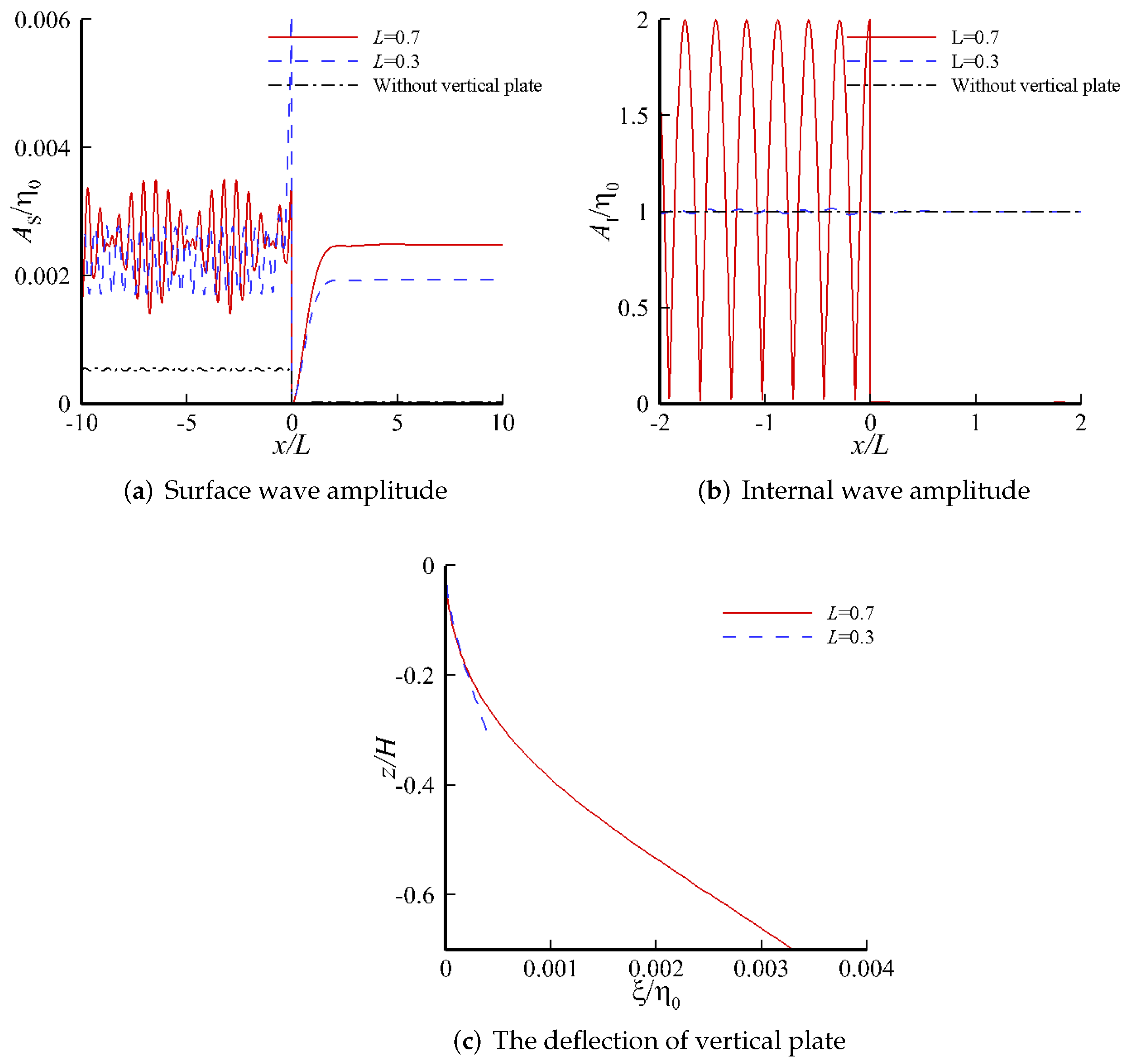
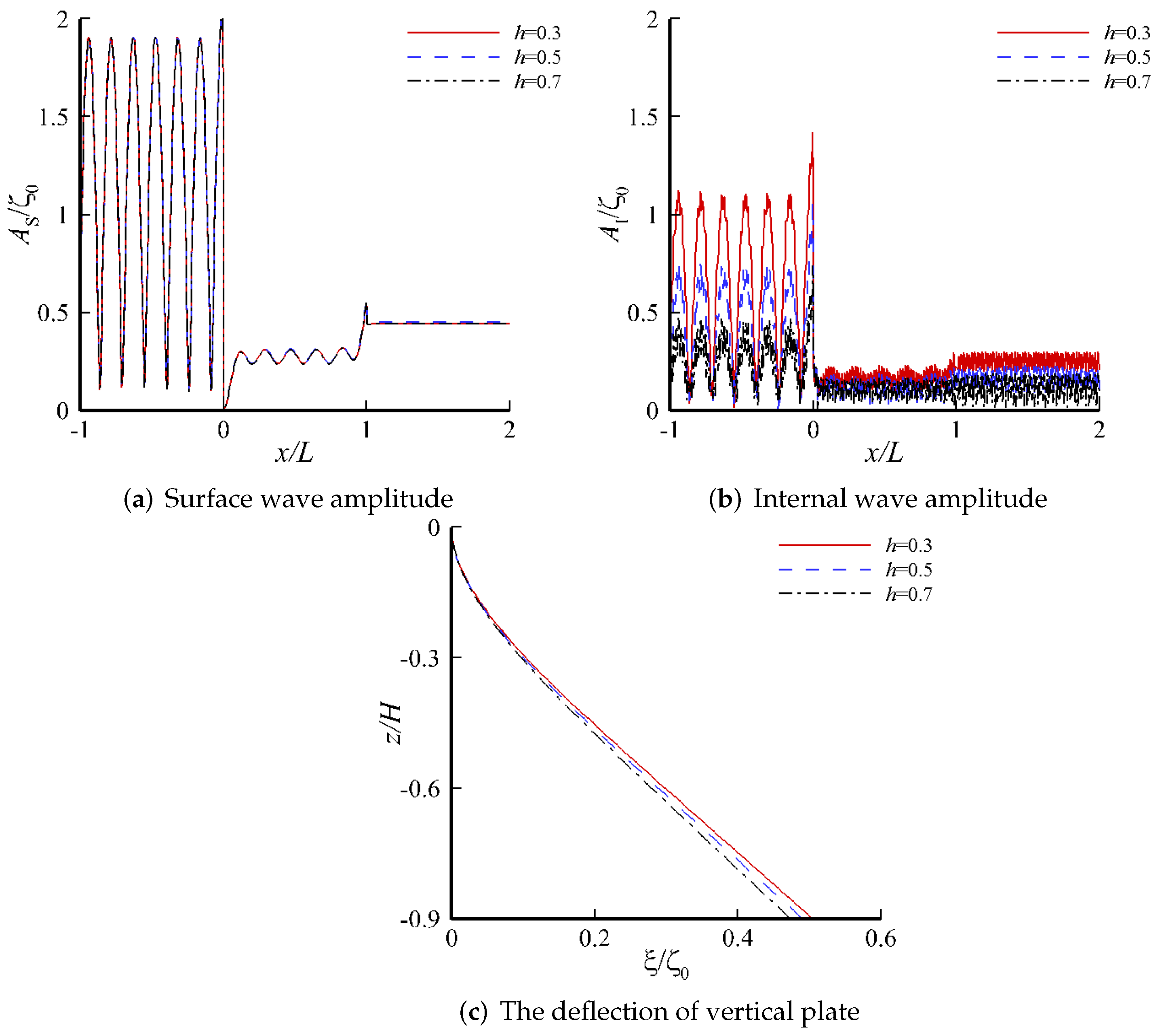
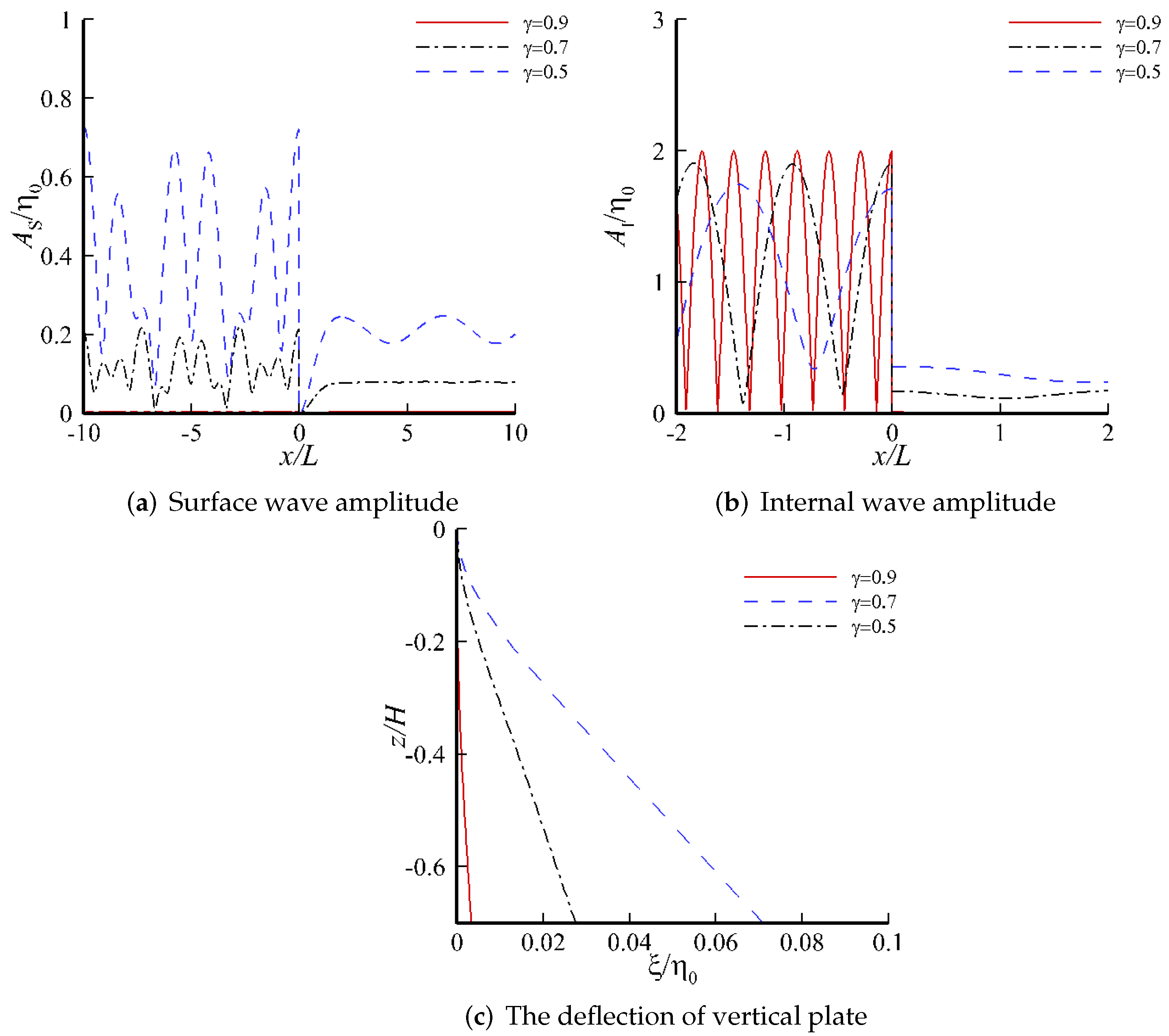
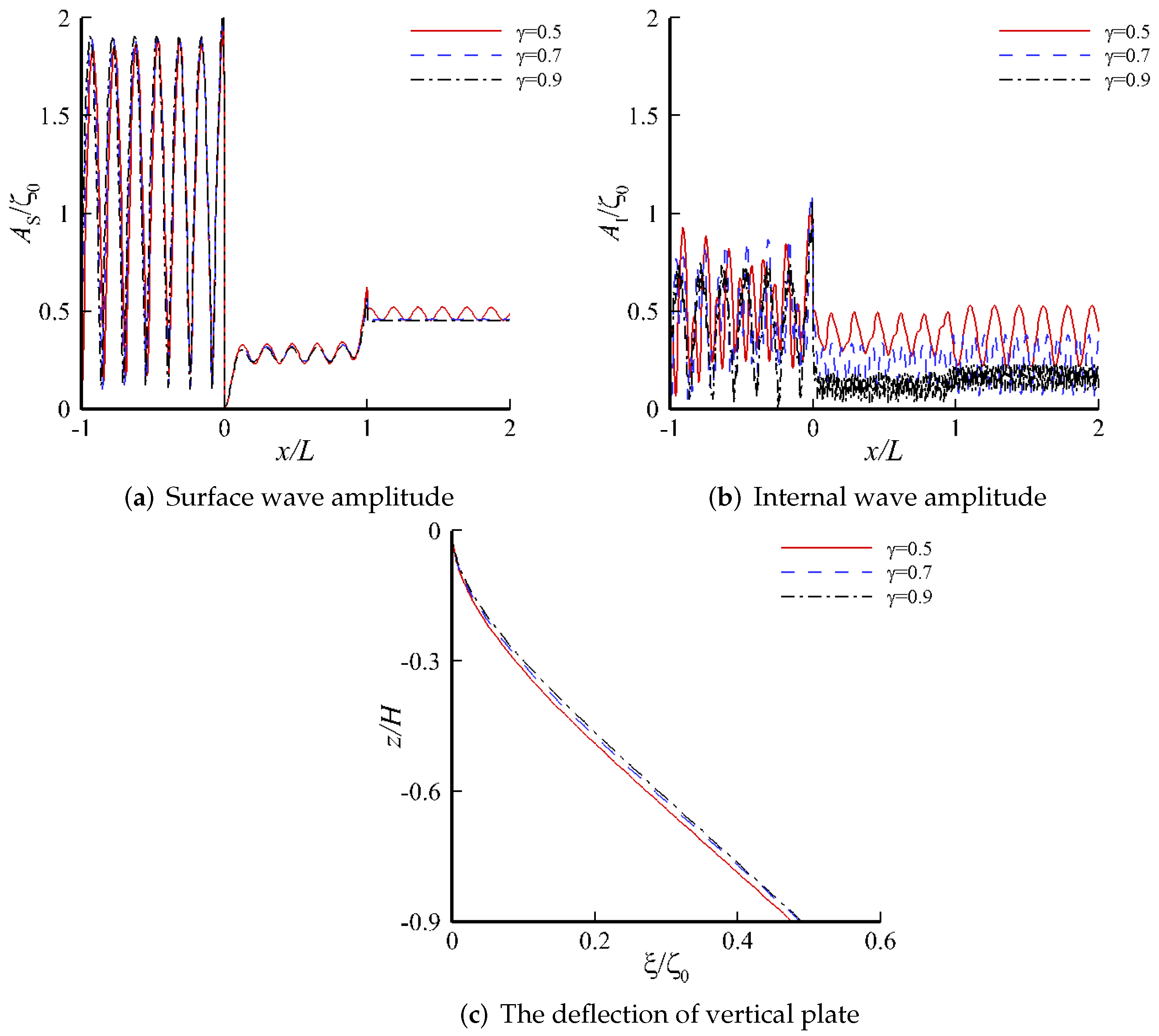
4.3. Response on the Two-Layer Fluid

In this section, we analyze the hydroelastic response on a two-layer fluid. We calculate the wave scattering due a semi-infinite plate and set ${\zeta }_0=0.01$, ${\eta }_0=0.0001$, $\gamma =0.9$, $h=0.5$, $G=0$, $L=0.9$, $\omega =1.25$, $L=12$, and $N=15$.

Figure 13 illustrates the variations of the amplitudes of surface and interfacial elevations versus x and the horizontal deflection of vertical plate versus z with different values of the porous-effect parameter G of the vertical porous flexible plate. It is similar to the situation in the single-layer fluid. The highest wave reflection and the lowest wave transmission are observed for the case with $G=0$. With the increment of the porous-effect parameter, the amplitude in the plate-covered and right open water region increase. With the introduction of porosity, the deflection of the wall decreases with the increment of porous-effect parameter G from Figure 13c. Thus, the main function of porosity is to reduce the load on the wall, and a medium porosity is a suitable choice to keep the balance between the reduction in the load and the suppression of the waves.

Figure 14 shows the variations of the amplitudes of surface and interfacial elevations versus x and the horizontal deflection of vertical plate versus z for different depth h of the interface. It is observed that, as h increases, the interfacial elevations decrease. The reason for this situation is that the wave energy decreases with a decreasing depth, and the wave energy in the interface is correspondingly reduced. The change of the surface amplitude with the increment of h is tiny enough to ignore. The deflection of the vertical plate changes slightly with the increment of h in Figure 14c. In general, the position of the interface has a small effect on the results.

Figure 15 illustrates the variations of the amplitudes of surface and interfacial elevations versus x and the horizontal deflection of vertical plate versus z for various values of L in the case of the incident waves of interfacial wave mode, where L is the length of the vertical plates. It reveals, in Figure 15a, that the interfacial incident wave has a small effects on the surface. Figure 15b shows the interfacial waves is mostly reflected by the vertical plate for $L=0.7$ when the vertical barrier pierces through the interface. The interfacial waves are almost unhindered for $L=0.3$.

Figure 16 shows the variations of the amplitudes of surface and interfacial elevations versus x and the horizontal deflection of vertical plate versus z for various values of $\gamma$ in the case of the incident waves of the interfacial wave mode, where $\gamma$ is the density ratio of the upper to the lower fluid layers. We set $\omega =0.75$ and $L=0.7$. Figure 16b shows that, with decrease in $\gamma$, the interfacial elevations decrease in the open region and increase in the plate-cover region. The interfacial incident wave has a small effect on the surface for $\gamma =0.9$ in Figure 16a. The amplitudes of the surface significantly increases with the decrement of $\gamma$. The deflection of the vertical plate also increases with the decrement of $\gamma$, as shown in Figure 16c.

Figure 17 demonstrates the variations of the amplitudes of surface and interfacial elevations versus x and the horizontal deflection of vertical plate versus z for various values of $\gamma$. Figure 17b shows that with the increase in $\gamma$, the interfacial elevations decrease, and it reveals that the density ratio significantly affects the wave amplitude in the interface. The amplitudes of surface remain almost the same for $\gamma =0.7$ and $\gamma =0.9$ in Figure 17a. In the case of $\gamma =0.5$, it is observed that the amplitudes of surface vary periodically due to the interfacial incident wave. The reason for the situation is that the energy of interfacial waves, according to the wave number displayed on the graph, transfers to surface and propagates in surface wave mode. The deflection of the vertical plate has little change due to the increment of $\gamma$, as shown in Figure 17c.

5. Conclusions

We have analytically studied the hydroelastic response of semi-infinite and finite floating elastic plate combined with a vertical elastic porous plate in a single-layer and a two-layer fluids with the aid of the method of matched eigenfunction expansions. The vertical plate is fixed to an edge of the floating plate and moored at its lower edge. The wave reflection and transmission by the structure was found to be strongly dependent on the length L and the porous effect parameter G of the vertical plate. Due to the low wave energy near the seabed, the changes of the curves between $L=0.7$ and $L=0.9$ is small, hence a further extension of the vertical plate has little effect on the solution. The vertical plate can decrease the bending moments and the shear forces on the floating plate.

The highest wave reflection and lowest wave transmission are observed for the case with the zero porous-effect parameter ($G=0$). For a higher porosity of the wall, more water will flow through the vertical plate. Thus, the amplitudes of surface and interfacial elevations increase as the value of G increases. The structural rigidity, the lateral stress and the mooring line angle of the vertical plate mainly affect the response of the vertical plate, and have a modest effect on the response of the floating plate. For a two-layer fluid system, the fluid density ratio and the position of interface mainly effect on the interfacial waves. As the lower position of interface descends, the interfacial amplitude decreases. When the vertical barrier pierces through the interface, the interfacial waves is mostly reflected by the vertical plate. With the decrease in $\gamma$, the interfacial incident waves have more effects on the surface. In particular, in the case of $\gamma =0.5$, the amplitudes of surface on the left open water region vary periodically due to the fact that the wave energy transfers from interfacial modes to surface ones and propagates in surface wave mode. The rate of energy flux in the results is approximatively conserved, and the method has high rate of convergence.

These observations are of significant importance in the design for eliminating the vibration of VLFS. Based on the discussion of the results presented here, we can conclude that, in order to keep a balance between the reduction in the wave loads on the wall and the suppression of the deflection on the VLFS, the addition of a submerged plate with the length of $L=0.7$ and a medium porous effect parameter is a suitable choice in design.

References

1. Watanabe, E.; Utsunomiya, T.; Wang, C.M. Hydroelastic analysis of pontoon-type VLFS: A literature survey. Eng. Struct. 2004, 26, 245–256. [Google Scholar] [CrossRef]
2. Andrianov, A.I. Hydroelastic Analysis of Very Large Floating Structures. Ph.D. Thesis, Delft University of Technology, Delft, The Netherlands, 2005. [Google Scholar]
3. Wang, C.M.; Tay, Z.Y. Very large floating structures: Applications, research and development. Procedia Eng. 2011, 14, 62–72. [Google Scholar] [CrossRef] [Green Version]
4. Lamas-Pardo, M.; Iglesias, G.; Carral, L. A review of Very large floating structures (VLFS) for coastal and offshore uses. Ocean Eng. 2015, 109, 677–690. [Google Scholar] [CrossRef]
5. Wang, C.M.; Tay, Z.Y.; Takagi, K.; Utsunomiya, T. Literature review of methods for mitigating hydroelastic response of VLFS under wave action. Appl. Mech. Rev. 2010, 63, 030802. [Google Scholar] [CrossRef]
6. Takagi, K.; Shimada, K.; Ikebuchi, T. An anti-motion device for a very large floating structure. Mar. Struct. 2000, 13, 421–436. [Google Scholar] [CrossRef]
7. Masanobu, S.; Kato, S.; Maeda, K.; Namba, Y. Response of the mega-float equipped with novel wave energy absorber. In Proceedings of the ASME 2003 22nd International Conference on Offshore Mechanics and Arctic Engineering, Cancun, Mexico, 8–13 June 2003; American Society of Mechanical Engineers Digital Collection: New York, NY, USA, 2003; pp. 727–734. [Google Scholar]
8. Lee, S.M.; Takaki, M.; Iwano, M. Estimation of the radiation forces on submerged-plate oscillating near a free surface by composite grid method. In Proceedings of the Transactions of the West-Japan Society of Naval Architects the 105th West-Japna Society of Naval Architects Meeting (Joint Autumn Meeting of Three Societies of Naval Architects in Japan); The Japan Society of Naval Architects and Ocean Engineers: Tokyo, Japan, 2003; pp. 113–122. Available online: https://www.jstage.jst.go.jp/article/wjsna/105/0/105_0_7/_article/-char/ja/ (accessed on 24 November 2021).
9. Pham, D.C.; Wang, C.M.; Utsunomiya, T. Hydroelastic analysis of pontoon-type circular VLFS with an attached submerged plate. Appl. Ocean. Res. 2008, 30, 287–296. [Google Scholar] [CrossRef]
10. Cheng, Y.; Ji, C.; Zhai, G.; Oleg, G. Dual inclined perforated anti-motion plates for mitigating hydroelastic response of a VLFS under wave action. Ocean Eng. 2016, 121, 572–591. [Google Scholar] [CrossRef]
11. Nguyen, H.; Wang, C.; Flocard, F.; Pedroso, D. Extracting energy while reducing hydroelastic responses of VLFS using a modular raft wec-type attachment. Appl. Ocean. Res. 2019, 84, 302–316. [Google Scholar] [CrossRef]
12. Nguyen, H.; Wang, C.; Luong, V. Two-mode WEC-type attachment for wave energy extraction and reduction of hydroelastic response of pontoon-type VLFS. Ocean Eng. 2020, 197, 106875. [Google Scholar] [CrossRef]
13. Feng, M.W.; Sun, Z.C.; Liang, S.X.; Liu, B.J. Hydroelastic response of VLFS with an attached submerged horizontal solid/porous plate under wave action. China Ocean Eng. 2020, 34, 451–462. [Google Scholar] [CrossRef]
14. Ohmatsu, S. Overview: Research on wave loading and responses of VLFS. Mar. Struct. 2005, 18, 149–168. [Google Scholar] [CrossRef]
15. Squire, V.A. Synergies between VLFS hydroelasticity and sea ice research. Int. J. Offshore Polar Eng. 2008, 18, 241–253. [Google Scholar]
16. Fox, C.; Squire, V.A. On the oblique reflexion and transmission of ocean waves at shore fast sea ice. Philos. Trans. R. Soc. Phys. Eng. Sci. 1994, 347, 185–218. [Google Scholar]
17. Sahoo, T.; Yip, T.L.; Chwang, A.T. Scattering of surface waves by a semi-infinite floating elastic plate. Phys. Fluids 2001, 13, 3215–3222. [Google Scholar] [CrossRef] [Green Version]
18. Xu, F.; Lu, D.Q. An optimization of eigenfunction expansion method for the interaction of water waves with an elastic plate. J. Hydrodyn. 2009, 21, 526–530. [Google Scholar] [CrossRef]
19. Xu, F.; Lu, D.Q. Wave scattering by a thin elastic plate floating on a two-layer fluid. Int. J. Eng. Sci. 2010, 48, 809–819. [Google Scholar] [CrossRef]
20. Meng, Q.R.; Lu, D.Q. Hydroelastic interaction between water waves and thin elastic plate floating on three-layer fluid. Appl. Math. Mech. - Engl. Ed. 2017, 38, 567–584. [Google Scholar] [CrossRef]
21. Yu, X.; Chwang, A.T. Wave-induced oscillation in harbor with porous breakwaters. J. Waterw. Port Coast. Ocean. Eng. 1994, 120, 125–144. [Google Scholar] [CrossRef]
22. Yip, T.L.; Sahoo, T.; Chwang, A.T. Trapping of surface waves by porous and flexible structures. Wave Motion 2002, 35, 41–54. [Google Scholar] [CrossRef]
23. Kumar, P.S.; Sahoo, T. Wave interaction with a flexible porous breakwater in a two-layer fluid. J. Eng. Mech. 2006, 132, 1007–1014. [Google Scholar] [CrossRef]
24. Mandal, S.; Behera, H.; Sahoo, T. Oblique wave interaction with porous, flexible barriers in a two-layer fluid. J. Eng. Math. 2016, 100, 1–31. [Google Scholar] [CrossRef]
25. Singla, S.; Martha, S.C.; Sahoo, T. Mitigation of structural responses of a very large floating structure in the presence of vertical porous barrier. Ocean Eng. 2018, 165, 505–527. [Google Scholar] [CrossRef]
Figure 1. Schematic diagram for the wave scattering by a semi-infinite elastic plate in a single-layer fluid.
Water 14 00294 g001
Figure 2. Schematic diagram in a two-layer fluid.
Water 14 00294 g002
Figure 3. Wave amplitudes A S ( x ) and deflection of vertical plate ξ ( z ) for the different number of terms N.
Water 14 00294 g003
Figure 4. Wave amplitudes A S ( x ) and deflection of vertical plate ξ ( z ) for the different length of vertical plate L.
Water 14 00294 g004
Figure 5. Wave amplitudes A S ( x ) and deflection of vertical plate ξ ( z ) with ω = 0.75 .
Water 14 00294 g005
Figure 6. Wave amplitudes A S ( x ) and deflection of vertical plate ξ ( z ) with ω = 1.25 .
Water 14 00294 g006
Figure 7. Wave amplitudes A S ( x ) and deflection of vertical plate ξ ( z ) with ω = 1.75 .
Water 14 00294 g007
Figure 8. Bending moment and shear force of the vertical and the horizonal plate.
Water 14 00294 g008
Figure 9. Wave amplitudes A S ( x ) and deflection of vertical plate ξ ( z ) for the different G.
Water 14 00294 g009
Figure 10. Wave amplitudes A S ( x ) and deflection of vertical plate ξ ( z ) for the different flexural rigidity D.
Water 14 00294 g010
Figure 11. Wave amplitudes A S ( x ) and deflection of vertical plate ξ ( z ) for the different lateral stress Q.
Water 14 00294 g011
Figure 12. Wave amplitudes A S ( x ) and deflection of vertical plate ξ ( z ) for the different mooring line angle θ .
Water 14 00294 g012
Figure 13. Wave amplitudes A S ( x ) and deflection of vertical plate ξ ( z ) for the different G.
Water 14 00294 g013
Figure 14. Wave amplitudes A S ( x ) , A I ( x ) , and deflection of vertical plate ξ ( z ) for the different depth ratio h.
Water 14 00294 g014
Figure 15. Wave amplitudes A S ( x ) , A I ( x ) , and deflection of vertical plate ξ ( z ) for the different length of a vertical plate L in the case of the incident waves of the interfacial wave mode.
Water 14 00294 g015
Figure 16. Wave amplitudes A S ( x ) , A I ( x ) and deflection of vertical plate ξ ( z ) for the different density ratio γ in the case of the incident waves of the interfacial wave mode.
Water 14 00294 g016
Figure 17. Wave amplitudes A S ( x ) , A I ( x ) and deflection of vertical plate ξ ( z ) for the different density ratio γ .
Water 14 00294 g017
Publisher’s Note: MDPI stays neutral with regard to jurisdictional claims in published maps and institutional affiliations.