
Predicting Snowmelt Runoff at the Source of the Mountainous Euphrates River Basin in Turkey for Water Supply and Flood Control Issues Using HEC-HMS Modeling


Abstract
:1. Introduction
2. Materials and Methods
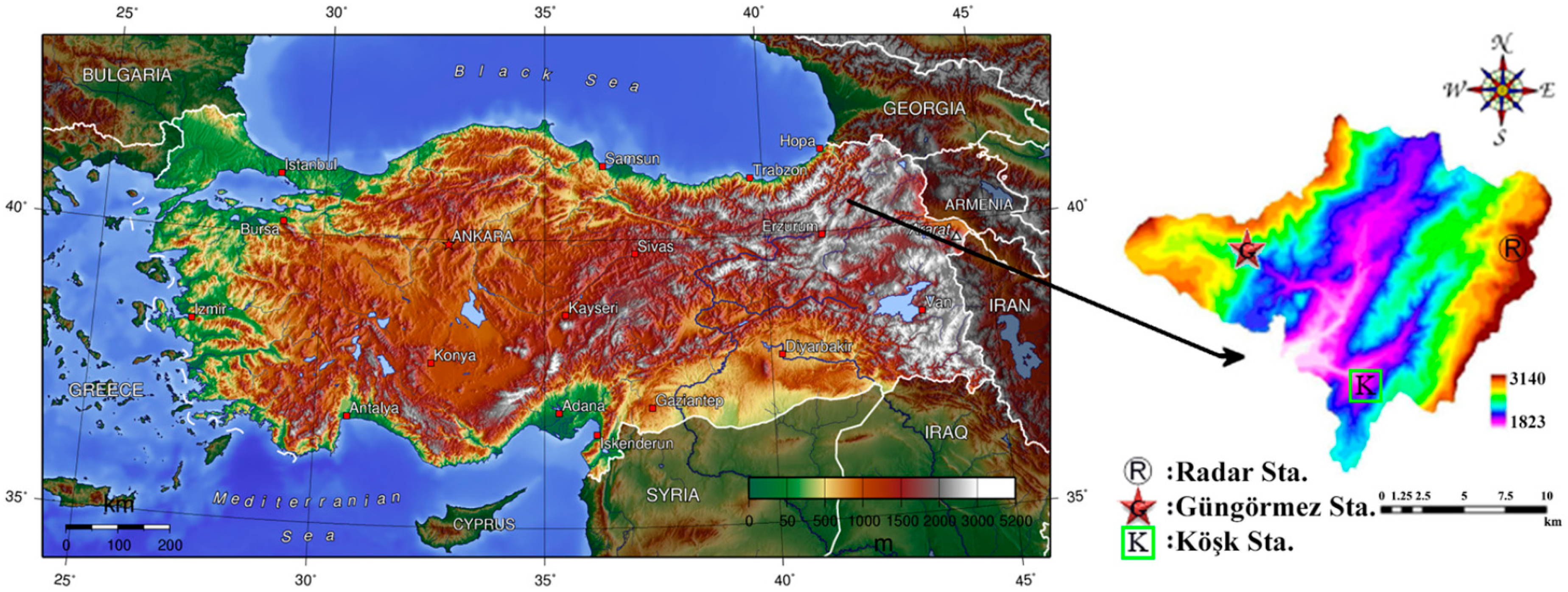
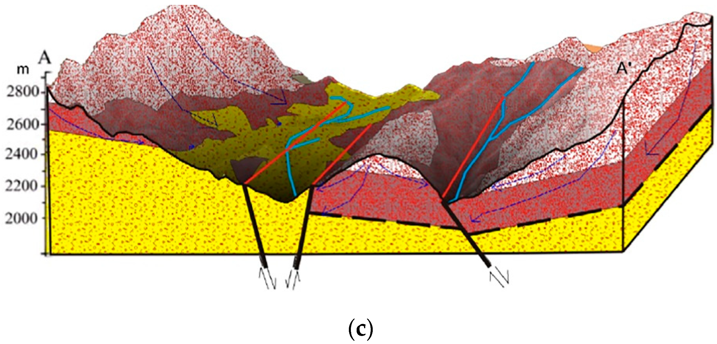
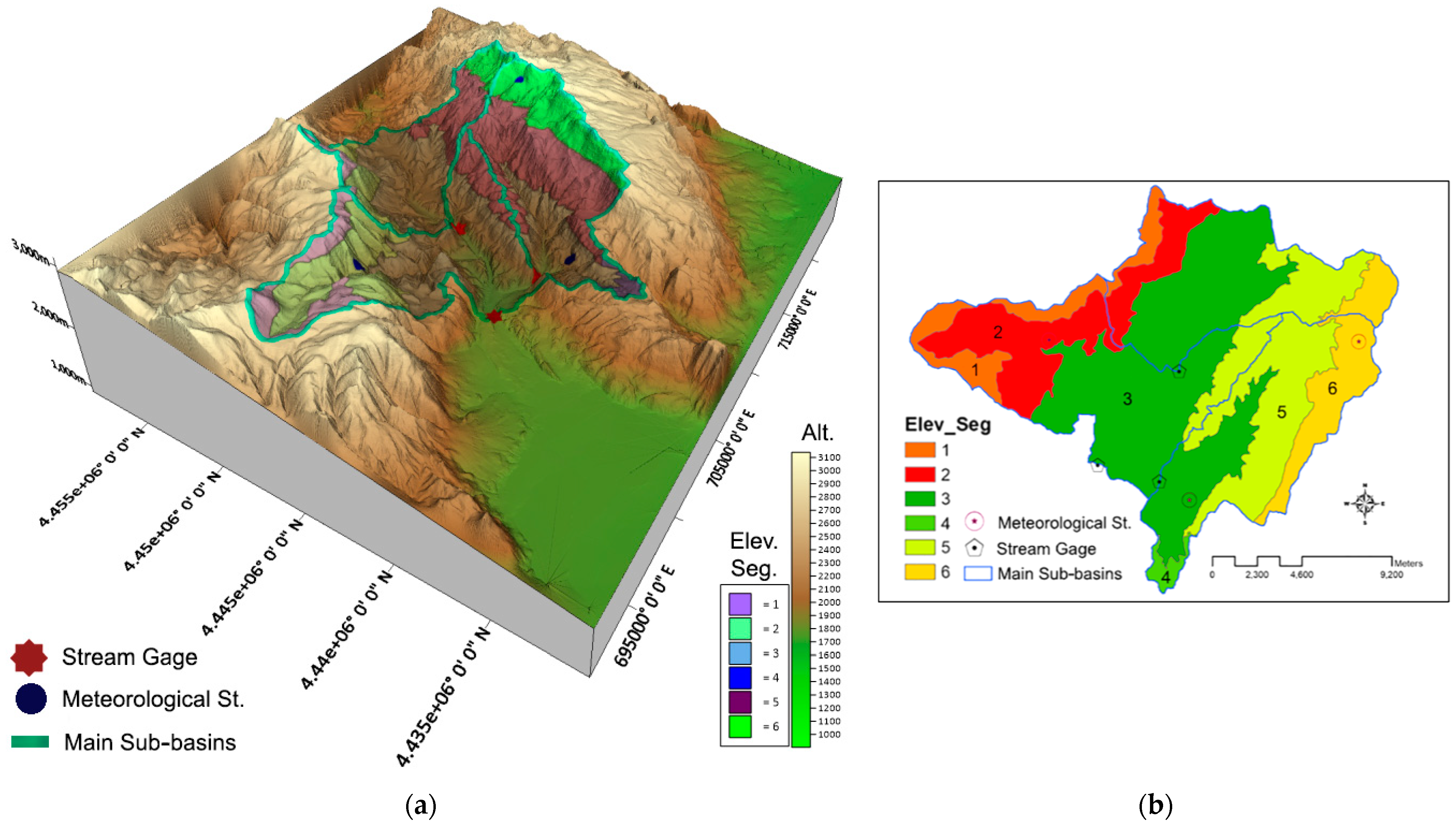
2.1. Area of Study
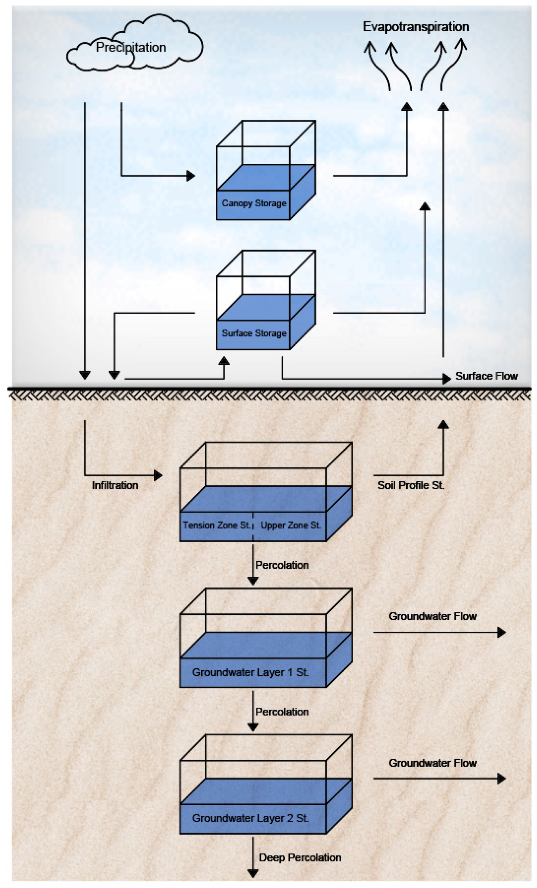
2.2. Hydrological Model
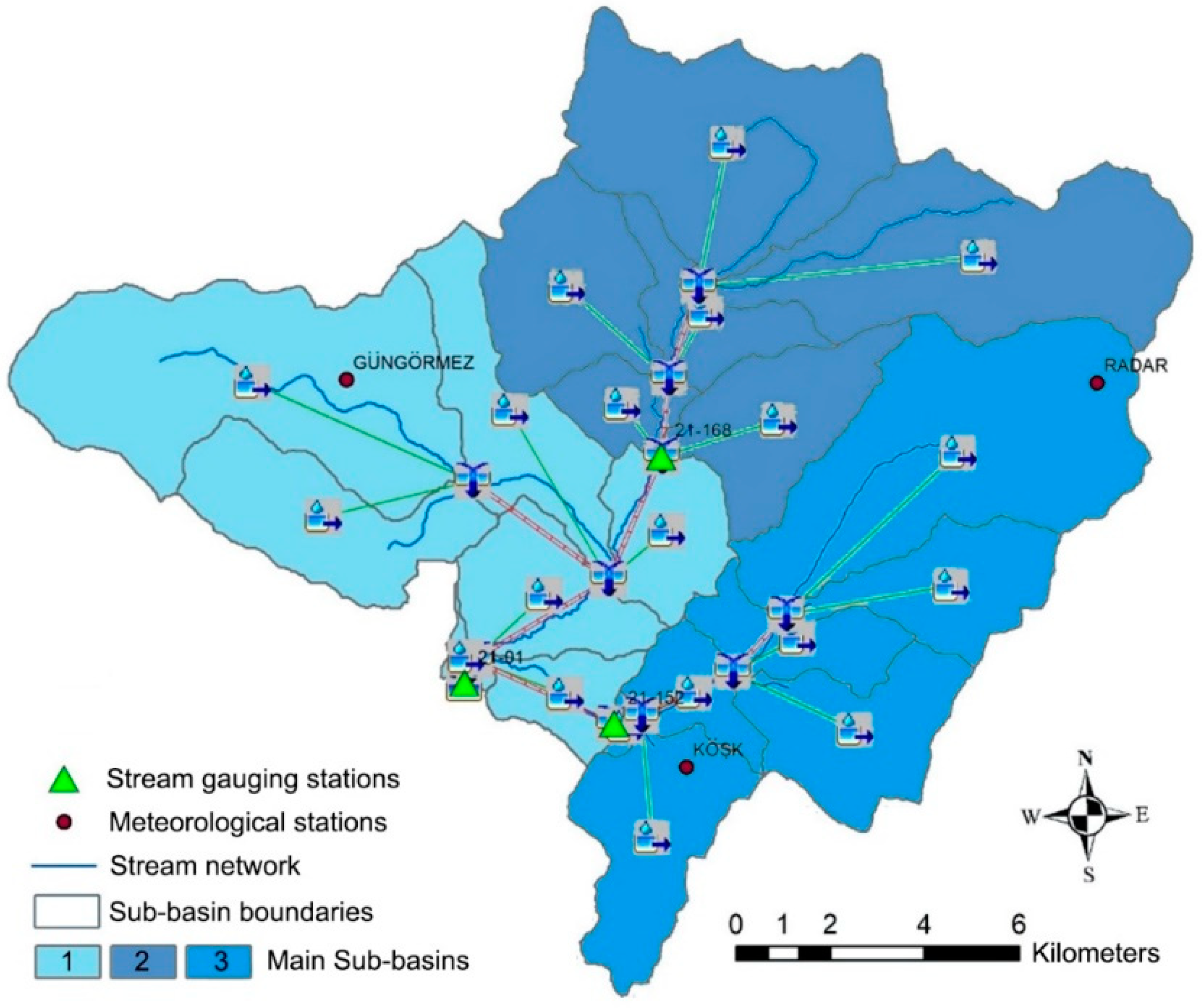
2.3. Basin Model
2.4. Meteorological Model
2.5. Precipitation Model
2.6. Snowmelt Model
2.7. Calibration Strategy
3. Results
4. Discussion
5. Conclusions
Author Contributions
Funding
Data Availability Statement
Conflicts of Interest
References
- Hassan, F. Water History for Our Times. In International Hydrological Programme; UNESCO: Paris, France, 2011; p. 122. [Google Scholar]
- Tekeli, A.E.; Akyürek, Z.; Arda Şorman, A.; Şensoy, A.; Ünal Şorman, A. Using MODIS Snow Cover Maps in Modeling Snowmelt Runoff Process in the Eastern Part of Turkey. Remote Sens. Environ. 2005, 97, 216–230. [Google Scholar] [CrossRef]
- Yucel, I.; Guventurk, A.; Sen, O.L. Climate Change Impacts on Snowmelt Runoff for Mountainous Transboundary Basins in Eastern Turkey. Int. J. Climatol. 2015, 35, 215–228. [Google Scholar] [CrossRef]
- Stewart, I.T. Changes in Snowpack and Snowmelt Runoff for Key Mountain Regions. Hydrol. Process. Int. J. 2009, 23, 78–94. [Google Scholar] [CrossRef]
- Sood, A.; Smakhtin, V. Global Hydrological Models: A Review. Hydrol. Sci. J. 2015, 60, 549–565. [Google Scholar] [CrossRef]
- Dong, C. Remote Sensing, Hydrological Modeling and in Situ Observations in Snow Cover Research: A Review. J. Hydrol. 2018, 561, 573–583. [Google Scholar] [CrossRef]
- Dhami, B.S.; Pandey, A. Comparative Review of Recently Developed Hydrologic Models. J. Indian Water Resour. Soc. 2013, 33, 34–41. [Google Scholar]
- Zhou, Y.; Cui, Z.; Lin, K.; Sheng, S.; Chen, H.; Guo, S.; Xu, C.-Y. Short-Term Flood Probability Density Forecasting Using a Conceptual Hydrological Model with Machine Learning Techniques. J. Hydrol. 2022, 604, 127255. [Google Scholar] [CrossRef]
- Wurbs, R.A. Dissemination of Generalized Water Resources Models in the United States. Water Int. 1998, 23, 190–198. [Google Scholar] [CrossRef]
- Yilmaz, A.G.; Imteaz, M.A.; Ogwuda, O. Accuracy of HEC-HMS and LBRM Models in Simulating Snow Runoffs in Upper Euphrates Basin. J. Hydrol. Eng. 2012, 17, 342–347. [Google Scholar] [CrossRef]
- Chen, Y.; Li, W.; Fang, G.; Li, Z. Review Article: Hydrological Modeling in Glacierized Catchments of Central Asia—Status and Challenges. Hydrol. Earth Syst. Sci. 2017, 21, 669–684. [Google Scholar] [CrossRef] [Green Version]
- Anderson, E.A. Snow Accumulation and Ablation Model–SNOW-17; NOAA’s National Weather Service Hydrology Laboratory NWSRFS User Manual; NOAA: Washington, DC, USA, 2006; p. 61. [Google Scholar]
- Zhou, J.; Pomeroy, J.W.; Zhang, W.; Cheng, G.; Wang, G.; Chen, C. Simulating Cold Regions Hydrological Processes Using a Modular Model in the West of China. J. Hydrol. 2014, 509, 13–24. [Google Scholar] [CrossRef] [Green Version]
- Samaniego, L.; Kumar, R.; Attinger, S. Multiscale Parameter Regionalization of a Grid-Based Hydrologic Model at the Mesoscale. Water Resour. Res. 2010, 46. [Google Scholar] [CrossRef] [Green Version]
- Burnash, R.J.C. The NWS River Forecast System—Catchment Modeling. In Computer Models of Watershed Hydrology; Water Resource Publication, LCC: Littleton, CO, USA, 1995; pp. 311–366. [Google Scholar]
- Speers, D.D. SSARR Model. In Computer Models of Watershed Hydrology; Water Resource Publication, LCC: Littleton, CO, USA; pp. 367–394.
- Scharffenberg, W.; Ely, P.; Daly, S.; Fleming, M.; Pak, J. Hydrologic Modeling System (HEC-HMS): Physically-Based Simulation Components. In Proceedings of the 2nd Joint Federal Interagency Conference, Las Vegas, NV, USA, 27 June–1 July 2010. [Google Scholar]
- USACE. Hydrologic Modeling System HEC-HMS User’s Manual; U.S. Army Corps of Engineers: Hanover, NH, USA, 2016.
- OHRG. Osisko Hammond Reef Gold Project, Hydrology Technical Support Document VERSION 2, Project Number: 13-1118-0010, Document Number: DOC018. 2013. Available online: https://www.ceaa-acee.gc.ca/050/documents/P63174/123081E.Pdf (accessed on 10 November 2021).
- Razmkhah, H.; Saghafian, B.; Ali, A.-M.A.; Radmanesh, F. Rainfall-Runoff Modeling Considnmering Soil Moisture Accounting Algorithm, Case Study: Karoon III River Basin. Water Resour. 2016, 43, 699–710. [Google Scholar] [CrossRef]
- Dariane, A.B.; Javadianzadeh, M.M.; James, L.D. Developing an Efficient Auto-Calibration Algorithm for HEC-HMS Program. Water Resour. Manag. 2016, 30, 1923–1937. [Google Scholar] [CrossRef]
- Darbandsari, P.; Coulibaly, P. Inter-Comparison of Lumped Hydrological Models in Data-Scarce Watersheds Using Different Precipitation Forcing Data Sets: Case Study of Northern Ontario, Canada. J. Hydrol. Reg. Stud. 2020, 31, 100730. [Google Scholar] [CrossRef]
- Kourgialas, N.N.; Karatzas, G.P.; Nikolaidis, N.P. An Integrated Framework for the Hydrologic Simulation of a Complex Geomorphological River Basin. J. Hydrol. 2010, 381, 308–321. [Google Scholar] [CrossRef]
- Fazel, K.; Scharffenberg, W.A.; Bombardelli, F.A. Assessment of the Melt Rate Function in a Temperature Index Snow Model Using Observed Data. J. Hydrol. Eng. 2014, 19, 1275–1282. [Google Scholar] [CrossRef]
- Şengül, S.; İspirli, M.N. Estimation and Analysis of the Antecedent Temperature Index–Melt Rate (ATIMR) Function Using Observed Data from the Kırkgöze-Çipak Basin, Turkey. J. Hydrol. 2021, 598, 126484. [Google Scholar] [CrossRef]
- Bombardelli, F.A.; García, M.H. Hydraulic Design of Large-Diameter Pipes. J. Hydraul. Eng. 2003, 129, 839–846. [Google Scholar] [CrossRef]
- Şorman, A.A.; Şensoy, A.; Tekeli, A.E.; Şorman, A.Ü.; Akyürek, Z. Modelling and Forecasting Snowmelt Runoff Process Using the HBV Model in the Eastern Part of Turkey. Hydrol. Process. 2009, 23, 1031–1040. [Google Scholar] [CrossRef]
- Yüksek, Ö. Reevaluation of Turkey’s Hydropower Potential and Electric Energy Demand. Energy Policy 2008, 36, 3374–3382. [Google Scholar] [CrossRef]
- Ogden, F.L.; Garbrecht, J.; DeBarry, P.A.; Johnson, L.E. GIS and Distributed Watershed Models. II: Modules, Interfaces, and Models. J. Hydrol. Eng. 2001, 6, 515–523. [Google Scholar] [CrossRef]
- Emerson, C.H.; Welty, C.; Traver, R.G. Watershed-Scale Evaluation of a System of Storm Water Detention Basins. J. Hydrol. Eng. 2005, 10, 237–242. [Google Scholar] [CrossRef]
- Leavesley, G.H.; Lichty, R.W.; Troutman, B.M.; Saindon, L.G. Precipitation-Runoff Modeling System: User’s Manual. Water-Resour. Investig. Rep. 1983, 83, 207. [Google Scholar]
- Akyürek, Z.; Şorman, A.Ü. Monitoring Snow-Covered Areas Using NOAA-AVHRR Data in the Eastern Part of Turkey. Hydrol. Sci. J. 2002, 47, 243–252. [Google Scholar] [CrossRef] [Green Version]
- Yerdelen, C.; Acar, R. Study on Prediction of Snowmelt Using Energy Balance Equations and Comparing with Regression Method in the Eastern Part of Turkey. J. Sci. Ind. Res. 2005, 64, 520–528. [Google Scholar]
- Şensoy, A.; Şorman, A.A.; Tekeli, A.E.; Şorman, A.; Garen, D.C. Point-scale Energy and Mass Balance Snowpack Simulations in the Upper Karasu Basin, Turkey. Hydrol. Process. Int. J. 2006, 20, 899–922. [Google Scholar] [CrossRef]
- Acar, R.; Şenocak, S.; Şengül, S. Snow Hydrology Studies in the Mountainous Eastern Part of Turkey. In Proceedings of the 2009 IEEE International Conference on Industrial Engineering and Engineering Management, Hong Kong, China, 8–11 December 2009; pp. 1578–1582. [Google Scholar]
- Acar, R.; Şenocak, S.; Şengül, S.; Coşkun, T.; Balık Şanlı, F. Erzurum Kırkgöze Havzasında Kar Erimesine Etki Eden Meteorolojik Ölçümlerin Üç İstasyonda Karşılaştırılması. In Proceedings of the III. Ulusal Kar Kongresi, Erzurum, Turkey, 17–19 February 2009. [Google Scholar]
- Şorman, A.A.; Uysal, G.; Şensoy, A. Probabilistic Snow Cover and Ensemble Streamflow Estimations in the Upper Euphrates Basin. J. Hydrol. Hydromech. 2019, 67, 82–92. [Google Scholar] [CrossRef] [Green Version]
- Şengül, S. Dağlık Havzalarda Hidrolojik Çevrime Etki Eden Parametrelerin Coğrafi Bilgi Sistemleri ve HSPF Model Programıyla İncelenmesi ve Kırkgöze Havzası Örneği. Ph.D. Thesis, Fen Bilimleri Enstitüsü, Atatürk Üniversitesi, Erzurum, Turkey, 2011. [Google Scholar]
- Şenocak, S. Kar Erimesi Akış Modelinin (SRM), Coğrafi Bilgi Sistemleri ve Uzaktan Algılama Teknikleri de Kullanılarak Dağlık Bölgelerde Uygulaması ve Erzurum Kırkgöze Havzası Örneği. Ph.D. Thesis, Fen Bilimleri Enstitüsü, Atatürk Üniversitesi, Erzurum, Turkey, 2011. [Google Scholar]
- İspirli, M.N. HEC-HMS Model Programı Kullanılarak Dağlık Havzalarda Kar Erimesine Etki Eden Parametrelerin Belirlenmesi ve Kırkgöze Çipak Havzası’nın Hidrolojik Modellenmesi Determination of Parameters Affecting Snow Melting in Mountain Basins Using HEC-HMS Model Program and Hydrologic Modeling of Kırkgöze Çıpak Basin. Master’s Thesis, Fen Bilimleri Enstitüsü, Atatürk Üniversitesi, Erzurum, Turkey, 2019. [Google Scholar]
- Şengül, S. Küresel İklim Değişikliğinin Yağış ve Sıcaklık Üzerindeki Etkilerinin Kırkgöze Dağlık Havzasındaki Kar Kütlesi Üzerinde 2050 Yılı İçin Beklenen Etkilerinin HSPF Model Programı İle İncelenmesi. Avrupa Bilim Ve Teknol. Derg. 2019, 17, 611–636. [Google Scholar]
- Akbulut, N.; Bayarı, S.; Akbulut, A.; Şahin, Y. Rivers of Turkey. In Rivers of Europe; Academic Press: London, UK, 2009; pp. 643–672. [Google Scholar]
- Pekkan, E. Yukarı Fırat Havzasında Kar Erimesi Sürecininuydu Görüntüsü Analizlerive Izleyici Teknikleri Ile Incelenmesi. Ph.D. Thesis, Fen Bilimleri Enstitüsü, Hacettepe Üniversitesi, Ankara, Turkey, 2009. [Google Scholar]
- Anonymous. Erzurum Projesi Mühendislik Jeolojisi Planlama Raporu; DSİ Genel Müdürlüğü; Jeoteknik Hizmetler ve Yeraltı Suları Dairesi Başkanlığı: Erzurum, Turkey, 1978; p. 48.
- Gyawali, R.; Watkins, D.W. Continuous Hydrologic Modeling of Snow-Affected Watersheds in the Great Lakes Basin Using HEC-HMS. J. Hydrol. Eng. 2013, 18, 29–39. [Google Scholar] [CrossRef]
- Chu, X.; Steinman, A. Event and Continuous Hydrologic Modeling with HEC-HMS. J. Irrig. Drain. Eng. 2009, 135, 119–124. [Google Scholar] [CrossRef]
- Scharffenberg, B. Introduction to HEC-HMS. In Proceedings of the Watershed Modeling with HEC-HMS, California Water and Engineering Forum, Sacramento, CA, USA, 28 May 2008. [Google Scholar]
- Khatri, H.B.; Jain, M.K.; Jain, S.K. Modelling of Streamflow in Snow Dominated Budhigandaki Catchment in Nepal. J. Earth Syst. Sci. 2018, 127, 100. [Google Scholar] [CrossRef] [Green Version]
- Viessman, W.J.; Lewis, G.L. Introduction to Hydrology; Addison Wesley Longman: Boston, MA, USA, 1995. [Google Scholar]
- USACE. Hydrologic Modeling System HEC-HMS Technical Reference Manual; U.S. Army Corps of Engineers: Hanover, NH, USA, 2000.
- Fortin, J.-P.; Turcotte, R.; Massicotte, S.; Moussa, R.; Fitzback, J.; Villeneuve, J.-P. Distributed Watershed Model Compatible with Remote Sensing and GIS Data. I: Description of Model. J. Hydrol. Eng. 2001, 6, 91–99. [Google Scholar] [CrossRef]
- Fleming, M.; Neary, V. Continuous Hydrologic Modeling Study with the Hydrologic Modeling System. J. Hydrol. Eng. 2004, 9, 175–183. [Google Scholar] [CrossRef]
- Khatami, S.; Khazaei, B. Benefits of GIS Application in Hydrological Modeling: A Brief Summary. Vatten Tidskr. För Vattenvård/J. Water Manag. Res. 2014, 70, 41–49. [Google Scholar]
- Donigian, A.S.; Davis, H.H. User’s Manual for Agricultural Runoff Management(ARM) Model; Environmental Protection Agency, Office of Research and Development, Environmental Research, Technology Development and Applications Branch: Washington, DC, USA, 1978.
- Bennett, T.H. Development and Application of a Continuous Soil Moisture Accounting Algorithm for the HEC-HMS. Master’s Thesis, Department of Civil and Environment Engineering, University of California, Davis, CA, USA, 1998. [Google Scholar]
- Balk, B.; Elder, K. Combining Binary Decision Tree and Geostatistical Methods to Estimate Snow Distribution in a Mountain Watershed. Water Resour. Res. 2000, 36, 13–26. [Google Scholar] [CrossRef]
- Erxleben, J.; Elder, K.; Davis, R. Comparison of Spatial Interpolation Methods for Estimating Snow Distribution in the Colorado Rocky Mountains. Hydrol. Process. 2002, 16, 3627–3649. [Google Scholar] [CrossRef]
- Cosgrove, B.A.; Lohmann, D.; Mitchell, K.E.; Houser, P.R.; Wood, E.F.; Schaake, J.C.; Robock, A.; Marshall, C.; Sheffield, J.; Duan, Q. Real-time and Retrospective Forcing in the North American Land Data Assimilation System (NLDAS) Project. J. Geophys. Res. Atmos. 2003, 108, D22. [Google Scholar] [CrossRef] [Green Version]
- Erickson, T.A.; Williams, M.W.; Winstral, A. Persistence of Topographic Controls on the Spatial Distribution of Snow in Rugged Mountain Terrain, Colorado, United States. Water Resour. Res. 2005, 41. [Google Scholar] [CrossRef] [Green Version]
- Molotch, N.P.; Colee, M.T.; Bales, R.C.; Dozier, J. Estimating the Spatial Distribution of Snow Water Equivalent in an Alpine Basin Using Binary Regression Tree Models: The Impact of Digital Elevation Data and Independent Variable Selection. Hydrol. Process. Int. J. 2005, 19, 1459–1479. [Google Scholar] [CrossRef]
- Liston, G.E.; Elder, K. A Meteorological Distribution System for High-Resolution Terrestrial Modeling (MicroMet). J. Hydrometeorol. 2006, 7, 217–234. [Google Scholar] [CrossRef] [Green Version]
- Liston, G.E.; Elder, K. A Distributed Snow-Evolution Modeling System (SnowModel). J. Hydrometeorol. 2006, 7, 1259–1276. [Google Scholar] [CrossRef] [Green Version]
- Winstral, A.; Marks, D. Long-term Snow Distribution Observations in a Mountain Catchment: Assessing Variability, Time Stability, and the Representativeness of an Index Site. Water Resour. Res. 2014, 50, 293–305. [Google Scholar] [CrossRef]
- Fassnacht, S.R.; Brown, K.S.J.; Blumberg, E.J.; Moreno, J.L.; Covino, T.P.; Kappas, M.; Huang, Y.; Leone, V.; Kashipazha, A.H. Distribution of Snow Depth Variability. Front. Earth Sci. 2018, 12, 683–692. [Google Scholar] [CrossRef]
- Jeong, H.-G.; Ahn, J.-B.; Lee, J.; Shim, K.-M.; Jung, M.-P. Improvement of Daily Precipitation Estimations Using PRISM with Inverse-Distance Weighting. Theor. Appl. Climatol. 2020, 139, 923–934. [Google Scholar] [CrossRef] [Green Version]
- Acar, R.; Sengul, S. The Estimation of Average Areal Snowfall by Conventional Methods and the Percentage Weighting Polygon Method in the Northeast Anatolia Region, Turkey. Energy Educ. Sci. Technol. Part A-Energy Sci. Res. 2012, 29, 11–22. [Google Scholar]
- Martinec, J.; Rango, A.; Roberts, R. Snowmelt Runoff Model User’s Manual; USDA Jornada Experimental Range, New Mexico State University: Las Cruces, NM, USA, 2008.
- USACE. Snow Hydrology; North Pacific Division; US Army Corps of Engineers: Portland, OR, USA, 1956.
- Martinec, J. The Degree-Day Factor for Snowmelt Runoff Forecasting. IUGG Gen. Assem. Hels. IAHS Comm. Surf. Waters 1960, 51, 468–477. [Google Scholar]
- Hock, R. Temperature Index Melt Modelling in Mountain Areas. J. Hydrol. 2003, 282, 104–115. [Google Scholar] [CrossRef]
- Davtalab, R.; Mirchi, A.; Khatami, S.; Gyawali, R.; Massah, A.; Farajzadeh, M.; Madani, K. Improving Continuous Hydrologic Modeling of Data-Poor River Basins Using Hydrologic Engineering Center’s Hydrologic Modeling System: Case Study of Karkheh River Basin. J. Hydrol. Eng. 2017, 22, 05017011. [Google Scholar] [CrossRef]
- Momblanch, A.; Holman, I.P.; Jain, S.K. Current Practice and Recommendations for Modelling Global Change Impacts on Water Resource in the Himalayas. Water 2019, 11, 1303. [Google Scholar] [CrossRef] [Green Version]
- Parajuli, A.; Nadeau, D.F.; Anctil, F.; Schilling, O.S.; Jutras, S. Does Data Availability Constrain Temperature-Index Snow Models? A Case Study in a Humid Boreal Forest. Water 2020, 12, 2284. [Google Scholar] [CrossRef]
- Kumar, M.; Marks, D.; Dozier, J.; Reba, M.; Winstral, A. Evaluation of Distributed Hydrologic Impacts of Temperature-Index and Energy-Based Snow Models. Adv. Water Resour. 2013, 56, 77–89. [Google Scholar] [CrossRef]
- He, Z.H.; Parajka, J.; Tian, F.Q.; Blöschl, G. Estimating Degree-Day Factors from MODIS for Snowmelt Runoff Modeling. Hydrol. Earth Syst. Sci. 2014, 18, 4773–4789. [Google Scholar] [CrossRef] [Green Version]
- Bobál, P.; Podhorányi, M.; Mudroň, I.; Holubec, M. Mathematical Modelling of the Dynamics of Mountain Basin Snow Cover in Moravian-Silesian Beskydy for Operational Purposes. Water Resour. 2015, 42, 302–312. [Google Scholar] [CrossRef]
- Bhuiyan, H.A.; McNairn, H.; Powers, J.; Merzouki, A. Application of HEC-HMS in a Cold Region Watershed and Use of RADARSAT-2 Soil Moisture in Initializing the Model. Hydrology 2017, 4, 9. [Google Scholar] [CrossRef] [Green Version]
- USACE. SSARR Model, Streamflow Synthesis and Reservoir Regulation. In User Manual; US Army Corps of Engineers: Portland, OR, USA, 1991. [Google Scholar]
- Bui, C. Application of HEC-HMS 3.4 in Estimating Streamflow of the Rio Grande under Impacts of Climate Change. Master’s Thesis, The University of New Mexico, Albuquerque, NM, USA, 2011. [Google Scholar]
- McEnroe, B.M. Guidelines for Continuous Simulation of Streamflow in Johnson County, Kansas, with HEC-HMS. Ph.D. Thesis, Department of Civil, Environmental and Architectural Engineering, University of Kansas, Lawrence, KS, USA, 2010. [Google Scholar]
- Bicknell, B.R.; Imhoff, J.C.; Kittle, J.L., Jr.; Jobes, T.H.; Donigian, A.S., Jr. Hydrological Simulation Program-Fortran (HSPF). User’s Manual for Release 12. US EPA National Exposure Research Laboratory, Athens, GA, in Cooperation with US Geological Survey; Water Resources Division: Reston, VA, USA, 2001.
- Knoben, W.; Freer, J.; Woods, R. Technical Note: Inherent Benchmark or Not? Comparing Nash-Sutcliffe and Kling-Gupta Efficiency Scores. Hydrol. Earth Syst. Sci. Discuss. 2019, 23, 4323–4331. [Google Scholar] [CrossRef] [Green Version]
- Krysanova, V.; Donnelly, C.; Gelfan, A.; Gerten, D.; Arheimer, B.; Hattermann, F.; Kundzewicz, Z.W. How the Performance of Hydrological Models Relates to Credibility of Projections under Climate Change. Hydrol. Sci. J. 2018, 63, 696–720. [Google Scholar] [CrossRef]
- Demirel, M.C.; Mai, J.; Mendiguren, G.; Koch, J.; Samaniego, L.; Stisen, S. Combining Satellite Data and Appropriate Objective Functions for Improved Spatial Pattern Performance of a Distributed Hydrologic Model. Hydrol. Earth Syst. Sci. 2018, 22, 1299–1315. [Google Scholar] [CrossRef] [Green Version]


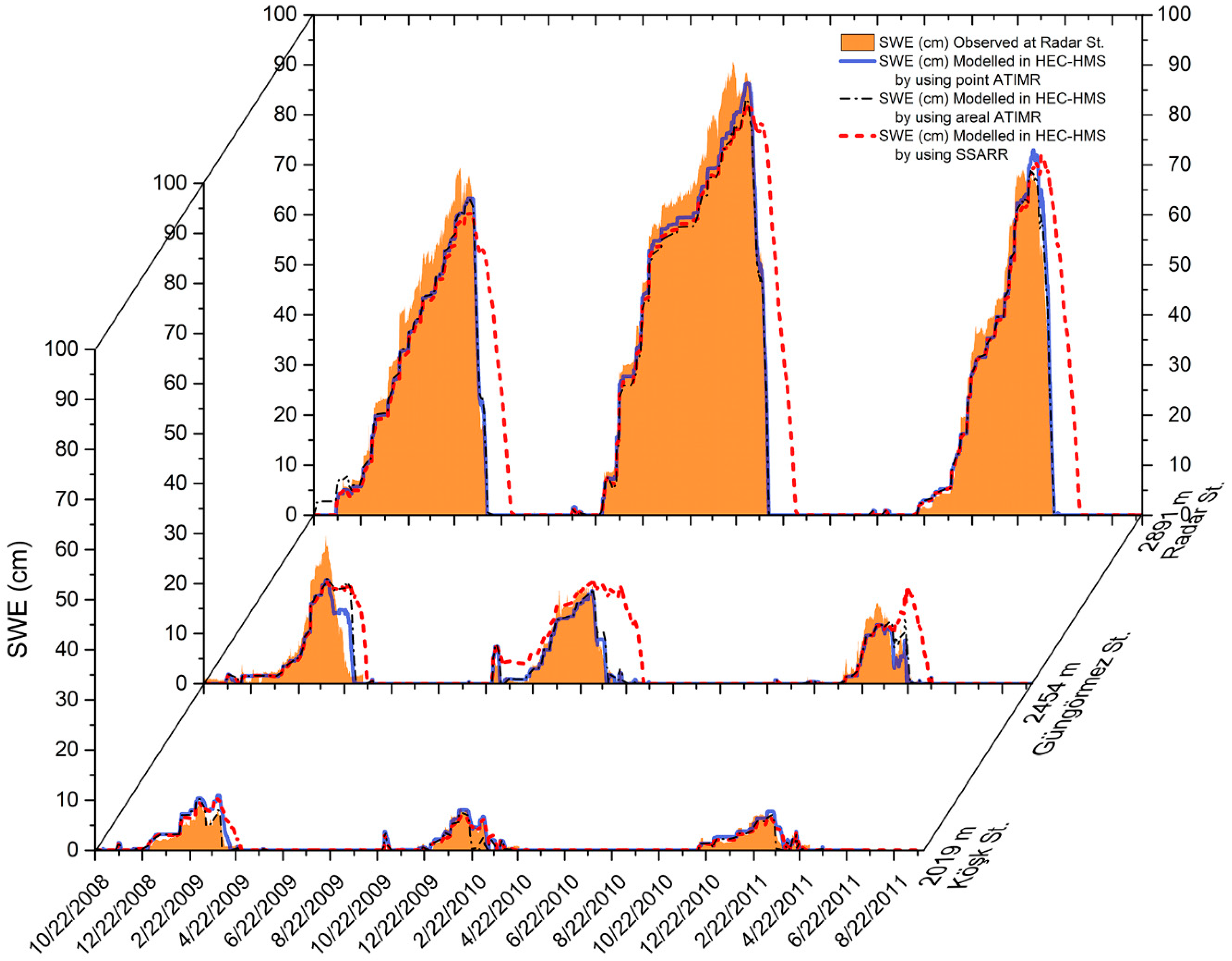
| Automatic Meteorology and Snow Observation Station | Altitude (m) | Aspect | Land Use | Average Slope of Land Close to the Station (Degrees) | Simulation Time Interval |
|---|---|---|---|---|---|
| KÖŞK | 2019 | Northwest | Dry Farming | 9.90 | 10/22/2008–9/30/2011 |
| GÜNGÖRMEZ | 2454 | Southeast | Transition Area | 24.10 | 10/22/2008–9/30/2011 |
| RADAR | 2891 | Northwest | Transition Area | 12.06 | 10/22/2008–9/30/2011 |
| MS1 | MS2 | MS3 | |
|---|---|---|---|
| Basin Slope (%) | 0.173 | 0.167 | 0.215 |
| Elevation (m) | 2125.02 | 2175.37 | 2204.53 |
| River Length (m) | 21,917.56 | 12,094.25 | 11,208.97 |
| Area (km2) | 91.53 | 75.50 | 74.51 |
| Zone | Hypsometric Elevation (m) | Weather Station | Weather Station Altitude (m) |
|---|---|---|---|
| 1 | 2777.236 | ||
| 2 | 2509.433 | Güngörmez | 2444 |
| 3 | 2098.651 | Köşk | 2042 |
| 4 | 2297.814 | ||
| 5 | 2454.838 | ||
| 6 | 2856.015 | Radar | 2887 |
| 1st Zone Calculated by extrapolating Köşk and Güngörmez station data | 1st Rule: If precipitation was observed at both stations, the total daily precipitation at the Köşk and Güngörmez stations was linearly extrapolated from the station altitudes to the average zone altitudes. If the extrapolation result was negative, the zonal precipitation altitude was taken as zero. (If Köşk > 0 and Güngörmez > 0, then the trend was applied. If the trend < 0, then 1st zone = 0). 2nd Rule: If there was no precipitation at Köşk but there was precipitation at the Güngörmez station, then precipitation altitude equals the Güngörmez station. (If Köşk = 0 and Güngörmez > 0, then 1st zone = Güngörmez). |
| 4th Zone Calculated by interpolating the Köşk and Radar station data | 1st Rule: If Köşk = 0, then 4th zone = 0. 2nd Rule: If Radar = 0, then 4th zone = Köşk. 3rd Rule: If Köşk > 0 and Radar > 0, then the trend is applied. If Trend < 0, then 4th zone = Köşk. |
| 5th Zone Calculated by extrapolating the Köşk and Radar station data | 1st Rule: If Köşk = 0 and Radar ≥ 5 mm, then the trend is applied. 2nd Rule: If Köşk = 0 and Radar < 5 mm, then 5th zone = 0. 3rd Rule: If Köşk < 5 mm and Radar = 0, then 5th zone = 0. 4th Rule: If Köşk ≥ 5 mm and Radar = 0, then the trend is applied by checking meteorological data from the Güngörmez and Radar stations. 5th Rule: If Köşk > 0 and Radar > 0, then the trend is applied. |
| ATIMR: °F-Day (°C-Day) | Melt Rate: in/°F-Day (cm/°C-Day) |
|---|---|
| 0 (0) | 0.025 (0.12) |
| 100 (55.56) | 0.03 (0.13) |
| 200 (111.11) | 0.05 (0.23) |
| 300 (166.67) | 0.04 (0.18) |
| 1000 (555.56) | 0.04 (0.18) |
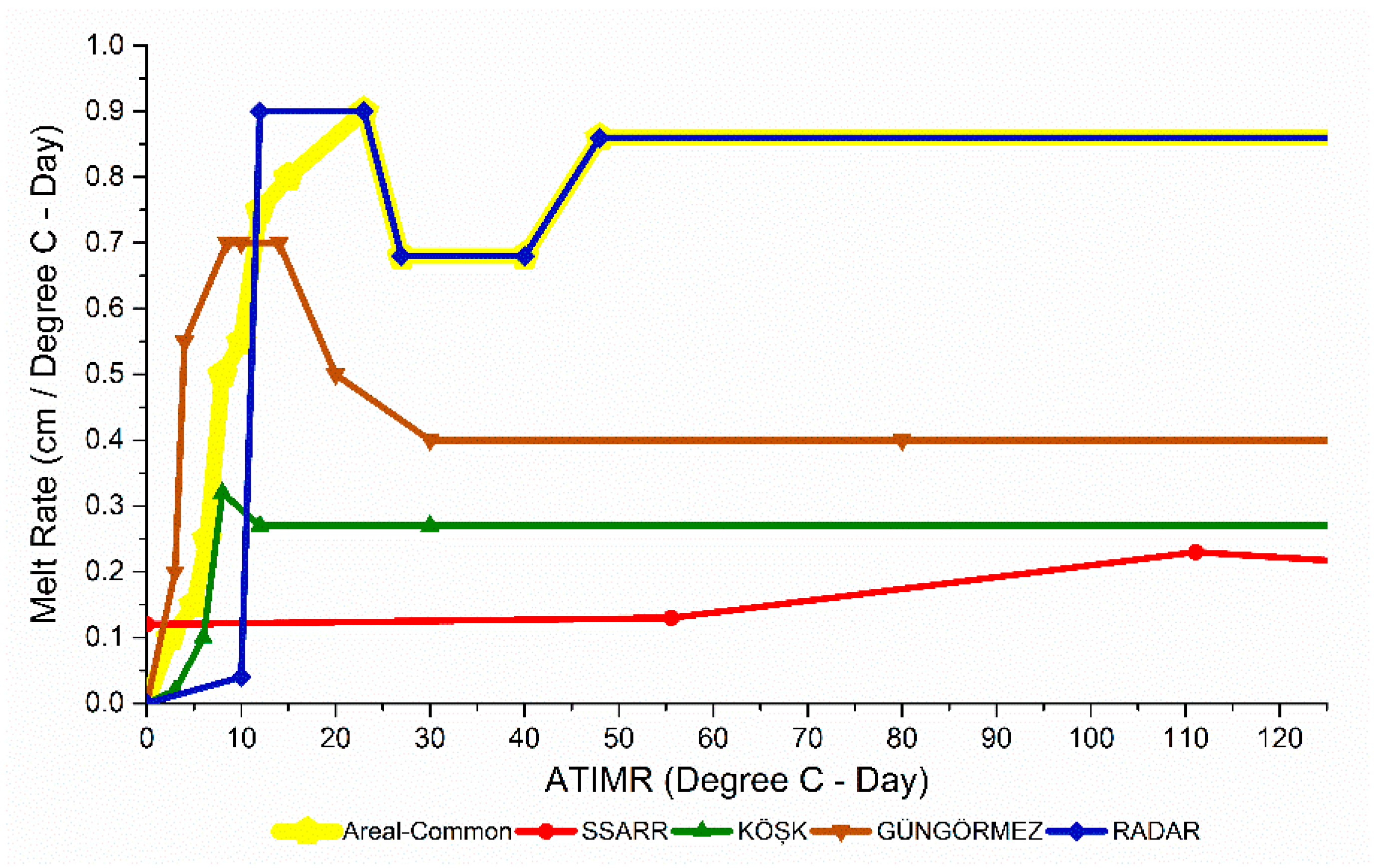
| Point ATIMR Curves | Areal-Common ATIMR Curve | ||||||
|---|---|---|---|---|---|---|---|
| Köşk Station (2019 m) | Güngörmez Station (2454 m) | Radar Station (2891 m) | Basin-Wide | ||||
| ATIMR (°C-Day) | Melt Rate (cm/°C-Day) | ATIMR (°C-Day) | Melt Rate (cm/°C-Day) | ATIMR (°C-Day) | Melt Rate (cm/°C-Day) | ATIMR (°C-Day) | Melt Rate (cm/°C-Day) |
| 0 | 0.00 | 0 | 0.00 | 0 | 0.00 | 0 | 0.00 |
| 3 | 0.02 | 3 | 0.02 | 10 | 0.04 | 2.5 | 0.10 |
| 6 | 0.10 | 4 | 0.55 | 12 | 0.90 | 5 | 0.15 |
| 8 | 0.32 | 8.5 | 0.70 | 23 | 0.90 | 6.4 | 0.25 |
| 12 | 0.27 | 10 | 0.70 | 27 | 0.68 | 8 | 0.50 |
| 30+ | 0.27 | 20 | 0.50 | 40 | 0.68 | 10 | 0.55 |
| 30 | 0.40 | 48 | 0.86 | 12 | 0.75 | ||
| 80+ | 0.40 | 125+ | 0.86 | 15 | 0.80 | ||
| 23 | 0.90 | ||||||
| 27 | 0.68 | ||||||
| 40 | 0.68 | ||||||
| 48 | 0.86 | ||||||
| 125+ | 0.86 | ||||||
| Station | Point R2 | Point RMSE (cm) | Point NSE | Point KGE | Area-Based R2 | Area-Based RMSE (cm) | Area-Based NSE | Area-Based KGE | SSARR R2 | SSARR RMSE (cm) | SSARR NSE | SSARR KGE | |
|---|---|---|---|---|---|---|---|---|---|---|---|---|---|
| Calibration period (2008–2010) | Köşk | 0.891 | 1.351 | 0.735 | 0.624 | 0.802 | 1.276 | 0.763 | 0.861 | 0.757 | 1.601 | 0.628 | 0.678 |
| Güngörmez | 0.887 | 2.610 | 0.876 | 0.830 | 0.770 | 3.591 | 0.766 | 0.857 | 0.385 | 7.312 | 0.030 | 0.322 | |
| Radar | 0.992 | 4.590 | 0.975 | 0.887 | 0.993 | 5.487 | 0.964 | 0.851 | 0.685 | 16.433 | 0.680 | 0.760 | |
| Validation period (2010–2011) | Köşk | 0.781 | 1.096 | 0.752 | 0.849 | 0.840 | 0.939 | 0.818 | 0.845 | 0.761 | 1.100 | 0.751 | 0.773 |
| Güngörmez | 0.922 | 1.834 | 0.874 | 0.730 | 0.814 | 2.235 | 0.812 | 0.871 | 0.230 | 6.207 | −0.449 | 0.246 | |
| Radar | 0.970 | 4.241 | 0.970 | 0.972 | 0.982 | 3.577 | 0.979 | 0.937 | 0.582 | 17.981 | 0.467 | 0.646 | |
| 3 years period (2008–2011) | Köşk | 1.280 | 0.858 | 0.740 | 0.701 | 0.805 | 1.185 | 0.777 | 0.874 | 0.730 | 1.469 | 0.658 | 0.779 |
| Güngörmez | 0.891 | 2.421 | 0.878 | 0.819 | 0.779 | 3.273 | 0.776 | 0.866 | 0.361 | 7.024 | −0.032 | 0.318 | |
| Radar | 0.985 | 4.476 | 0.976 | 0.904 | 0.989 | 4.931 | 0.970 | 0.868 | 0.666 | 16.966 | 0.648 | 0.758 |
| Sub-Model | Method | Parameter | MS1 (Inc. 8 Sub-Basins) | MS2 (Inc. 5 Sub-Basins) | MS3 (Inc. 5 Sub-Basins) | |||
|---|---|---|---|---|---|---|---|---|
| Initial | Calibrated | Initial | Calibrated | Initial | Calibrated | |||
| Canopy | Simple Canopy | Initial Storage (%) | 0 | 0 | 0 | 0 | 0 | 0 |
| Max. Storage (mm) | 2.5 | 6.77 | 2.5 | 4.23 | 2.5 | 5.97 | ||
| Surface | Simple Surface | Initial Storage (%) | 0 | 0 | 0 | 0 | 0 | 0 |
| Max. Storage (mm) | 5 | 6.67 | 5 | 6.67 | 5 | 6 | ||
| Loss | Soil Moisture Accounting | Max. Infiltration (mm/h) | 2 | 1.208 | 2 | 1.95 | 2 | 1.73 |
| Impervious (%) | 0 | 0 | 0 | 0 | 0 | 0 | ||
| Soil Storage (mm) | 100 | 71.93 | 100 | 101.83 | 100 | 66.97 | ||
| Tension Storage (mm) | 50 | 41.25 | 50 | 33.55 | 50 | 45.64 | ||
| Soil Percolation (mm/h) | 0.6 | 0.06 | 0.6 | 0.06 | 0.6 | 0.06 | ||
| GW1 Storage (mm) | 30 | 33.33 | 30 | 33.33 | 30 | 26.67 | ||
| GW1 Percolation (mm/h) | 0.4 | 3.55 | 0.4 | 3.55 | 0.4 | 2.84 | ||
| GW1 Coefficient (h) | 300 | 541.67 | 300 | 361.11 | 300 | 511.11 | ||
| GW2 Storage (mm) | 40 | 35 | 40 | 35 | 40 | 35 | ||
| GW2 Percolation (mm/h) | 0.3 | 2.67 | 0.3 | 2.67 | 0.3 | 2.13 | ||
| GW2 Coefficient (h) | 400 | 433.33 | 400 | 288.88 | 400 | 408.88 | ||
| Transform | Clark Unit Hydrograph | Time of Concentration (h) | 2.386 | 2.386 | 2.528 | 2.529 | 2.176 | 2.175 |
| Storage Coefficient (h) | 200 | 80 | 200 | 80 | 200 | 300 | ||
| Base Flow | Constant Monthly | January (m3/s) | 0.048 | 0.048 | 0.065 | 0.065 | 0.056 | 0.056 |
| February (m3/s) | 0.074 | 0.074 | 0.099 | 0.099 | 0.079 | 0.079 | ||
| March (m3/s) | 0.121 | 0.121 | 0.158 | 0.158 | 0.143 | 0.143 | ||
| April (m3/s) | 0.183 | 0.183 | 0.221 | 0.221 | 0.233 | 0.233 | ||
| May (m3/s) | 0.226 | 0.226 | 0.205 | 0.205 | 0.272 | 0.272 | ||
| June (m3/s) | 0.123 | 0.092 | 0.133 | 0.099 | 0.161 | 0.241 | ||
| July (m3/s) | 0.084 | 0.063 | 0.097 | 0.072 | 0.112 | 0.126 | ||
| August (m3/s) | 0.062 | 0.046 | 0.075 | 0.056 | 0.080 | 0.060 | ||
| September (m3/s) | 0.054 | 0.041 | 0.067 | 0.050 | 0.071 | 0.053 | ||
| October (m3/s) | 0.053 | 0.053 | 0.067 | 0.067 | 0.069 | 0.069 | ||
| November (m3/s) | 0.050 | 0.050 | 0.065 | 0.065 | 0.064 | 0.064 | ||
| December (m3/s) | 0.046 | 0.046 | 0.060 | 0.060 | 0.058 | 0.058 | ||
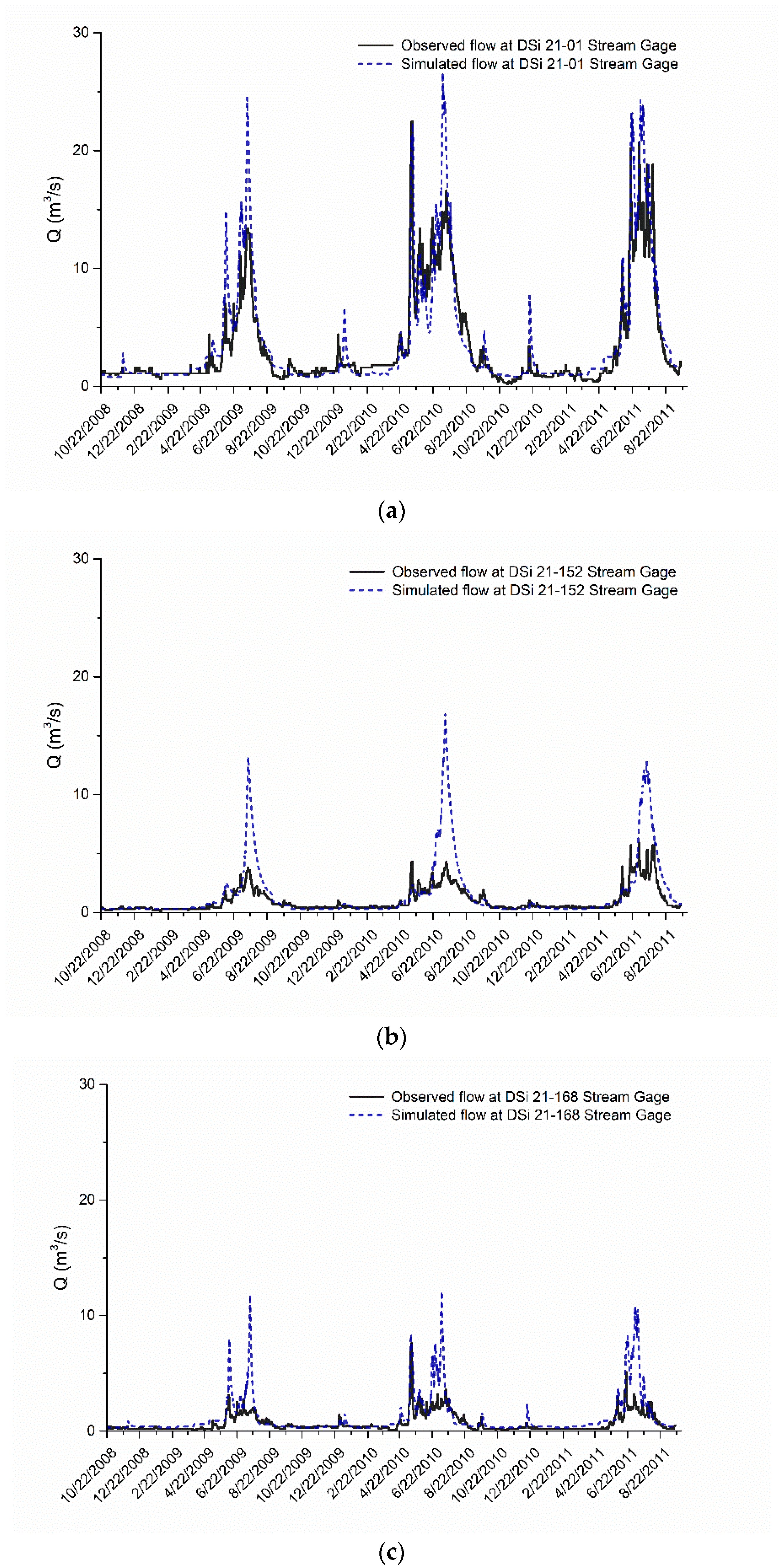
| Station | R2 | RMSE | NSE | KGE |
|---|---|---|---|---|
| 21-01 (Karasu-Çipak) | 0.840 | 2.144 | 0.817 | 0.748 |
| 21-152 (Köşk Dere-Köşk) | 0.656 | 1.967 | 0.431 | 0.262 |
| 21-168 (Büyükçay-Karagöbek) | 0.586 | 1.359 | 0.406 | 0.265 |
Publisher’s Note: MDPI stays neutral with regard to jurisdictional claims in published maps and institutional affiliations. |
© 2022 by the authors. Licensee MDPI, Basel, Switzerland. This article is an open access article distributed under the terms and conditions of the Creative Commons Attribution (CC BY) license (https://creativecommons.org/licenses/by/4.0/).
Share and Cite
Şengül, S.; İspirli, M.N. Predicting Snowmelt Runoff at the Source of the Mountainous Euphrates River Basin in Turkey for Water Supply and Flood Control Issues Using HEC-HMS Modeling. Water 2022, 14, 284. https://doi.org/10.3390/w14030284
Şengül S, İspirli MN. Predicting Snowmelt Runoff at the Source of the Mountainous Euphrates River Basin in Turkey for Water Supply and Flood Control Issues Using HEC-HMS Modeling. Water. 2022; 14(3):284. https://doi.org/10.3390/w14030284
Chicago/Turabian StyleŞengül, Selim, and Muhammet Nuri İspirli. 2022. "Predicting Snowmelt Runoff at the Source of the Mountainous Euphrates River Basin in Turkey for Water Supply and Flood Control Issues Using HEC-HMS Modeling" Water 14, no. 3: 284. https://doi.org/10.3390/w14030284
APA StyleŞengül, S., & İspirli, M. N. (2022). Predicting Snowmelt Runoff at the Source of the Mountainous Euphrates River Basin in Turkey for Water Supply and Flood Control Issues Using HEC-HMS Modeling. Water, 14(3), 284. https://doi.org/10.3390/w14030284