Article

Evaluating a Surface Energy Balance Model for Partially Wetted Surfaces: Drip and Micro-Sprinkler Systems in Hazelnut Orchards (Corylus Avellana L.)

1
Departamento de Recursos Hídricos, Facultad de Ingeniería Agrícola, Universidad de Concepción, Chillán 3812120, Chile
2
Centro de Recursos Hídricos Para la Agricultura y Minería (CRHIAM), Universidad de Concepción, Chillán 3812120, Chile
3
Horticultural Crops Production and Genetic Improvement Research Unit, U.S. Department of Agriculture, Agricultural Research Service, 3420 NW Orchard Avenue, Corvallis, OR 97330, USA
4
U.S. Fulbright Program—Chile, Universidad de Concepción, Chillán 3812120, Chile
5
Environmental Engineering & Biotechnology Group (GIBA-UDEC), Environmental Science Faculty, Universidad de Concepción, Concepcion 4070386, Chile
*
Author to whom correspondence should be addressed.
Water 2022, 14(24), 4011; https://doi.org/10.3390/w14244011
Submission received: 10 September 2022 / Revised: 19 November 2022 / Accepted: 5 December 2022 / Published: 8 December 2022
(This article belongs to the Section Soil and Water)

Abstract

:
A multi-layer surface energy balance model was previously developed to estimate crop transpiration (T) and soil evaporation (E) in orchards partially wet by micro-irrigation systems. The model, referred to as SEB-PW, estimates latent (λE), sensible (H), and soil heat fluxes (G) and separates actual evapotranspiration (ETa) into dry and wet soil E and crop T. The main goal of this work was to evaluate the ability of the SEB-PW model to estimate ETa and analyze the diurnal and seasonal dynamics of E and T in two hazelnut (Corylus avellana L.) orchards irrigated by drip or micro-sprinkler systems. The assessment showed that simulated hourly ET was highly correlated with estimates from nearby weather stations and with measurements from micro-lysimeters (MLs). Hourly ET estimates were evaluated by root-mean-square error (RMSE), mean absolute error (MAE), the Nash–Sutcliffe coefficient (NSE), and the index of agreement (da), which equaled 58.6 W m−2, 35.6 W m−2, 0.85, and 0.94, respectively. Daily E estimates were also evaluated and equaled 0.27 mm day−1, 0.21 mm day−1, 0.87, and 0.94, respectively, and obtained a coefficient of determination (r2) of 0.85 when compared to the measurements from the MLs. Within a day of irrigation, E accounted for 28 and 46% of ET. In accordance with the obtained results, the proposed SEB-PW model improves estimates of soil E by allowing the wetted and non-wetted areas to be estimated separately, which could be useful for optimizing irrigation methods and practices in hazelnut orchards.

Graphical Abstract

1. Introduction

Hazelnut (Corylus avellana L.) is an important tree nut crop, with a global production of roughly 1,072,000 tons of in-shell nuts per year and a cultivated area of approximately 1,015,000 ha [1]. Most production of the crop occurs in Turkey (70%), Italy (11%), the United States, Georgia, and Azerbaijan [2,3]. Chile is also becoming a significant producer, where the area planted with hazelnuts has increased exponentially from 2500 ha to 24,456 ha in the last 10 years and is predicted to continue to increase at a rate of 3000 ha per year [4,5]. Soon, Chile will play a major role in the international hazelnut market and could become one of the largest exporters of the crop worldwide [3].
Irrigation is often essential in hazelnuts, particularly in areas with limited rainfall or in soils with low water holding capacity. The trees are susceptible to water stress due to poor stomatal regulation [6] and require approximately 800 mm of supplemental rain or irrigation per season to fully develop [7]. Water stress reduces photosynthetic activity quickly in hazelnuts and can result in early termination of fruit growth, earlier leaf drop, and a higher incidence of disease in the crop [8,9,10,11]. Usually, hazelnut orchards are irrigated by drip or micro-sprinkler systems, which, if designed and managed properly, have excellent uniformity and high application efficiencies.
Knowing the exact amount of water required by a crop is essential for irrigation planning and for improving the efficiency of irrigation water use. Low-volume systems such as drip or micro-sprinklers typically have lower wetted surface areas than other irrigation methods (e.g., sprinklers), which, depending on the frequency of water applications, can lead to less soil evaporation (E) [12]. Estimates in almond orchards have shown that evapotranspiration (ET) is 10% to 15% higher with micro-irrigation systems than with surface or sprinkler systems [13]. Depending on the type of irrigation system used, soil E can be a significant component of total crop ET during the growing season [14,15]. E from bare soil is commonly described in two stages [16]. During the first stage, E is governed by atmospheric conditions and is limited by available energy in the upper soil layers and by the vapor gradient between the soil and atmosphere. During the second stage, E primarily becomes a function of soil water content, soil hydraulic properties, and temperature gradients [17].
Studies have shown that E can range between 10% to 70% of ET for different crop types, including grapes and olives [18,19,20,21]. Even in drip-irrigated vineyards, E can represent 28% to 46% of total ET after an irrigation event [14]. For crops with lower spacing densities, such as hazelnuts (570–800 trees ha−1), E may constitute an even greater fraction of total ET due to the larger area of soil surface exposed directly to sunlight and the atmosphere. In hazelnut, previous studies have focused on water consumption [7,22,23], but the separation of ET into soil E and canopy transpiration (T) has not been reported to our knowledge.
Different approaches are used for the determination of ET. Traditionally, ET is determined by multiplying reference ET, usually obtained from an automated weather station, by a set of seasonal crop coefficients. Crop coefficients are determined according to crop type and growth stage and normally follow the FAO-56 procedure [24]. However, this method requires information on the dates of crop development, which can sometimes be difficult to predict due to the different geographic and climate zones where a crop is planted [25]. Another commonly accepted method is the Penman–Monteith model. Modifications to the Penman–Monteith model consist of extending the single-layer model to a multi-layer model, such as two layers in the Shuttleworth and Wallace model [26] and four layers in the Choudhury and Monteith model [27], where crop-to-crop differences are represented by crop-specific surface and aerodynamic resistance values [28,29]. The multi-layer models partition the available energy into latent heat (λE), sensible heat (H), and soil heat (G) fluxes for the canopy/soil system and offer the possibility of including the effect of partially wetted surfaces on total ET [14]. The advantage of these models for determining total ET, T, and E is widely recognized [30,31,32,33,34,35,36,37,38].
A modified surface energy balance model was previously proposed by Souto et al. [14] to estimate actual evapotranspiration (ETa). The model uses a surface energy balance for partially wetted (SEB-PW) orchards irrigated by micro-irrigation systems and includes the effect of E from wetted and non-wetted areas on total ET. The model is based on the original approaches of Lagos et al. [29] and Choudhury and Monteith [27] and has the advantage of partitioning ET into T and E. The model was initially evaluated in a drip-irrigated wine grape vineyard in Northern California for a range of fractional crop canopy cover conditions; however, further evaluation is required to test the model in other crops, including hazelnut.
The main goal of the present work was to evaluate the ability of the SEB-PW model to estimate total ETa, crop T, and soil E in hazelnut and analyze the diurnal and seasonal dynamics of T and E in orchards irrigated by drip or micro-sprinklers. Estimated hourly, diurnal, and seasonal ETa were compared with estimated ET obtained from two ET stations, as well as with E measurements from micro-lysimeters (MLs), during three growing seasons in the southern Central Valley of Chile.

2. Materials and Methods
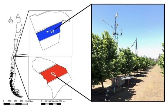
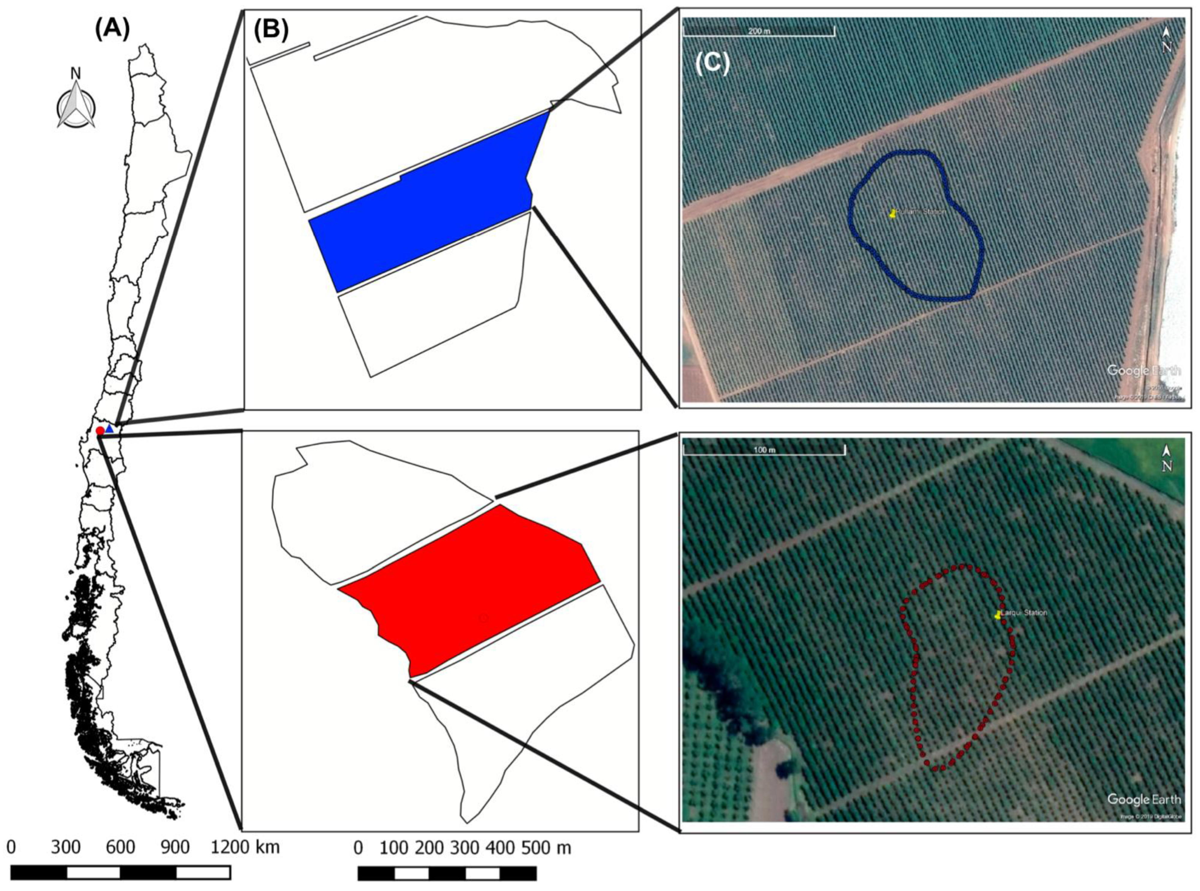
2.1. Study Site

The SEB-PW model was applied at two commercial hazelnut orchard sites, S1 and S2, which are located 20 km east of the city of Chillán (36°35′20.07″ S, 71°47′55.51″ W; 254 m above sea level) and 5 km west of the city of Bulnes (36°42′30.53″ S, 72°21′38.25″ W; 72 m above sea level) in the Diguillin Province, Ñuble Region of Chile, respectively (Figure 1). In both cases, the model was evaluated during the 2017–2018, 2018–2019, and 2020–2021 growing seasons. The soil at the sites consisted mainly of deep clay and clay loam, respectively. Site S1 was planted with the cultivar Tonda di Giffoni and irrigated by one micro-sprinkler (GyroNet, Netafim USA, Fresno, CA, USA) per tree. Each micro-sprinkler had a nominal flow rate of 30 L h−1. Irrigation, in this case, was scheduled 6 days per week in November and December, 5 days per week in January and February, and 7 days per week in March. Site S2 was planted with the cultivar Lewis and irrigated with two laterals per row and four drip emitters (Netafim USA, Fresno, CA, USA) per tree. Each drip emitter had a nominal flow rate of 3.8 L h−1. Drip irrigation was scheduled every 2–3 days for the entire growing season. Irrigation was similar each growing season and was controlled by the farmers at the sites. Other characteristics of the sites are presented in Table 1.
The orchards were harvested at the sites between the second half of March and the first half of April each year. The yield was measured during normal harvesting operations using blocks of trees located within the footprint areas of each ET station (see ‘ET and Micrometeorological Measurements’). Nuts were harvested manually and then collected in buckets and weighed. Yield totaled 5000, 5215, and 5150 kg ha−1 of fresh nuts in 2018, 2019, and 2021, respectively, at site S1, and 5450, 5983, and 5750 kg ha−1 of fresh nuts in 2018, 2019, and 2021, respectively, at site S2. Canopy height increased over time at the sites and ranged from 3.5–4.0 m in 2017–2018, 4.0–4.5 m in 2018–2019, and 4.5–5.0 in 2020–2021.

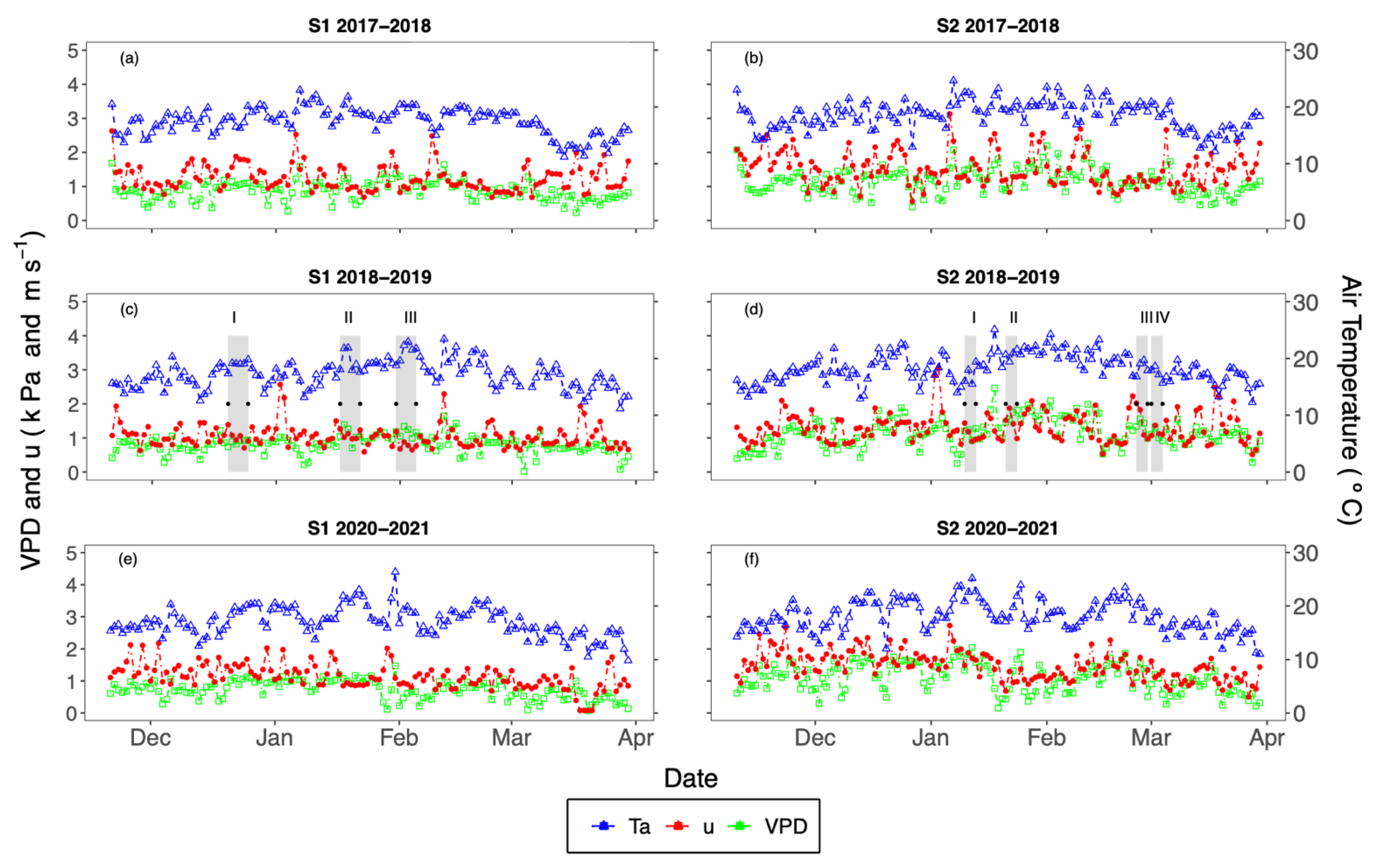
2.2. Climatic Conditions at the Study Site

The climate in the area of the study sites is typically warm and temperate, with the average temperature ranging from 27.8 in January to 3.4 °C in July [39]. During this study, air temperatures averaged 17.5, 17.2, and 17.4 °C during the 2017–2018, 2018–2019, and 2020–2021 growing seasons, respectively, at site S1 and 18.5, 18.2, and 18.3 °C during the 2017–2018, 2018–2019, and 2020–2021 growing seasons, respectively, at site S2. Annual rainfall at the sites totaled 1083 mm in 2017–2018, 776 mm in 2018–2019, and 710 mm in 2020–2021; average wind speed measured at 5.0 m and height ranged between 1.1 and 1.5 m s−1, with a predominant direction from the southeast at S1 and the southwest at S2. See Figure 2 for daily changes in average air temperature, wind speed, and vapor pressure deficit. Reference ET at the sites was approximately 670, 750, and 720 mm in the 2017–2018, 2018–2019, and 2020–2021 growing seasons, respectively.

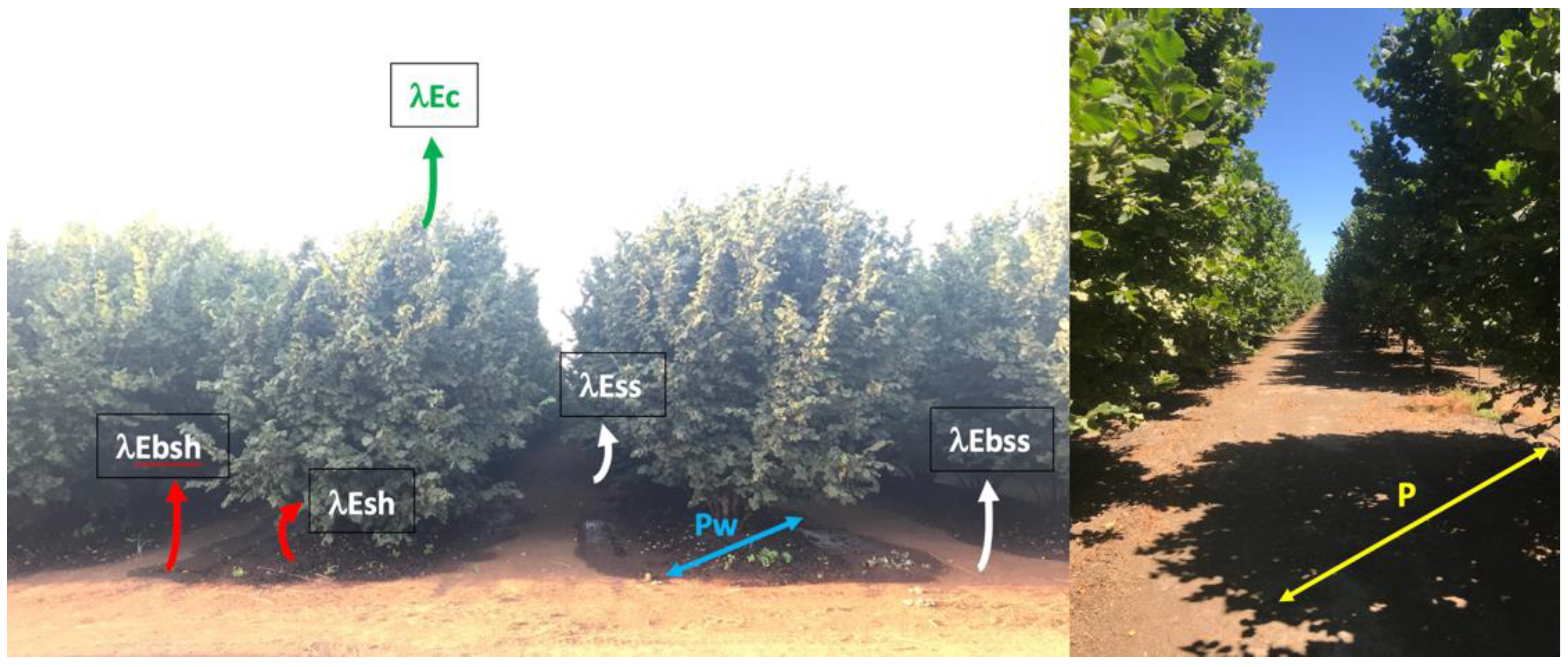
2.3. The Modified SEB-PW Model

A modified surface energy balance model, SEB-PW, was used in the present study. The model has four layers, including the interaction of irrigated and non-irrigated areas, and distributes net radiation (Rn) into latent and sensible heat (λE and H), as well as soil heat (G) fluxes through the soil-canopy system, according to the energy balance. The total Rn, H, G, and λE fluxes are calculated rather than adding a wet soil fraction (Pw) in the SEB-PW model (see Figure 3). A summary of the SEB-PW model can be reviewed in Appendix A.

2.4. ET and Micrometeorological Measurements

A micro weather station (ET station) was installed at each site to measure the SEB components and micro-meteorological variables at 30 min intervals using a data logger (CR3000, Campbell Scientific Inc., Logan, UT, USA). Components included: two net radiometers (NRLite2, Kipp and Zonen Inc., Delft, the Netherlands) to measure Rn at 1.5 m above the canopy and at 3.0 m above the bare soil (between rows); a three-dimensional sonic anemometer (81000, R.M. Young Inc., Traverse City, MI, USA) mounted at ≈ 2.0 m above the canopy to measure H; two soil sensor packages each with two soil heat flux plates (HFP01SC, Hukseflux, Delft, the Netherlands), one soil moisture sensor (CS616, Campbell Scientific Inc., Logan, UT, USA), and four soil temperature probes (TCAV, Campbell Scientific Inc., Logan, UT, USA) to calculate G. For each package, the lower heat flux plate was installed horizontally at a depth 0.08 m below the soil surface, the soil moisture sensor was installed at a depth of 0.03 m, and the temperature probes were installed at depths of 0.02 m to 0.06 m on both sides of the heat flux plate and the soil moisture sensor. One package was installed in a tree row, and the other was located between two rows; G was calculated using the mean of both measurements. λE was determined using the SEB method, which estimates the values as the residual from Rn, H, and G. Each ET station also included a rain gauge (TR-525M, Texas Electronics, Dallas, TX, USA) and an air temperature/relative humidity probe (EE181-L Probe, Campbell Scientific Inc., Logan, UT, USA). These sensors were mounted ≈1.0 m above the canopy.
The shaded soil fraction (P) beneath the canopy was measured once a month from October to March on days with clear skies at solar noon (±1 h). Leaf area index (LAI) was calculated using the method developed by Allen et al. [25] using images from the Sentinel-2A satellite. The methodology was programmed in Google Earth Engine (GEE).

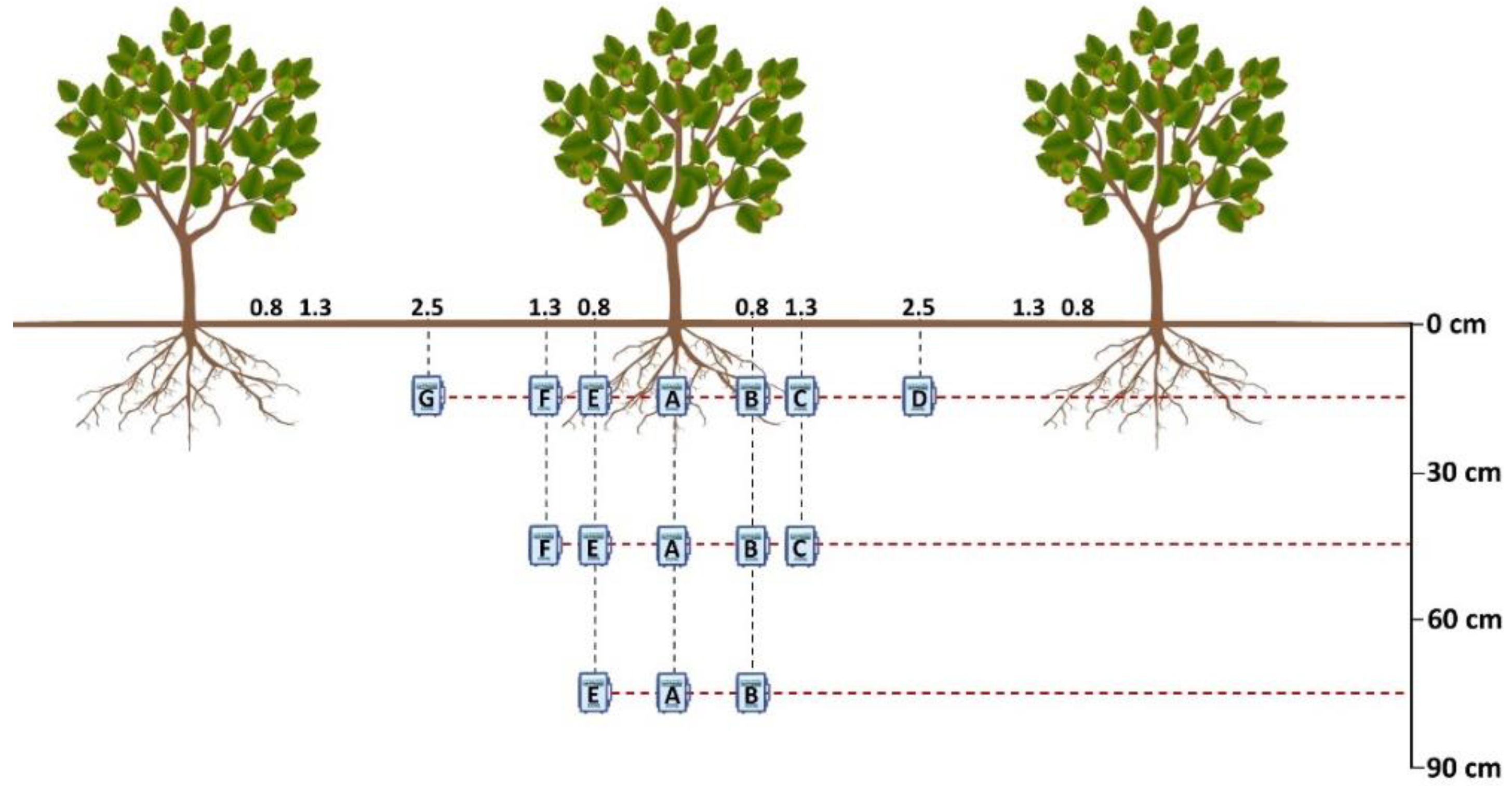
2.5. Soil Moisture Measurements

Soil water tension (SWT) was measured with a set of 12 solid-state electric resistance sensors (Watermark, Irrometer Company, Inc., Riverside, CA, USA). The sensors were placed at depths of 0.15, 0.45, and 0.75 m within and around the root system of a representative tree at both sites (Figure 4). Readings from the sensors were collected every 30 min using a data logger (900 M, Irrometer Company, Inc., Riverside, CA, USA). The wet soil fraction (Pw) on the surface was measured daily between 9:00 and 10:00 AM during three or four field campaigns in 2018–2019 (see Figure 2). The measurements were carried out with a measuring tape and then correlated to irrigated and non-irrigated areas recorded by the Watermark sensors.

2.6. Soil Evaporation Measurements

Soil E was measured using MLs, following procedures described by Feng et al. [40]. The MLs were manufactured from stainless steel rings with a height of 0.1 m and a diameter of 0.082 m (cross-sectional area of 0.00528 m2). A layer of PVC insulation was used to minimize lateral heat flux between the soil inside and outside the MLs [41]. Sixteen MLs were installed at site S1, including four each in wetted and non-wetted areas between the rows and below the canopy, and twelve MLs were installed at site S2, including six between rows (non-wetted area) and six below the canopy (wetted areas). Each ML was installed ≈24 h after irrigation, after which undisturbed soil cores were collected using stainless steel rings. The samples were capped at the bottom before being placed in a PVC sleeve and weighed every day between 8:00 and 9:00 AM and between 7:00 and 8:00 PM using an electronic scale (Gram FC-2000, Gram group, Barcelona, Spain) with a precision of 0.01 g. Each set of measurements was taken in the morning and evening to differentiate diurnal and nightly E values, i.e., when Rn was positive just after sunrise and before sunset. Measurements at site S1 were performed during three field campaigns, each lasting 5 days, during the period between 20 December 2018 and 23 January 2019. Measurements at site S2 were performed during four field campaigns, each lasting 2 days, during the period between 11 January and 3 March 2019.

2.7. Footprint Analysis

To ensure that the fluxes measured by the ET station came mainly from the surface of interest, the area of influence (footprint) at each site was calculated at both sites using the model proposed by Kljun et al. [42]. The calculations showed that 90% of the fluxes measured using the EC method were mainly from the area of interest (blue and red circled areas in Figure 1C). The recorded datasets revealed the main flux measurement inputs came primarily from southern to southeastern areas at site S1 and from southern to southwestern areas at site S2. The total area covered by the footprints was in the range of 100–140 m in width (east to west) and 150–200 m in length (north to south) at S1 and in the range of 50–70 m in width (east to west) and 100–120 m in length (north to south) at S2. The data used for modeling covered the entire growing season in 2017–2018, 2018–2019, and 2020–2021.

2.8. Model Performance

To assess the performance of the proposed model, five statistical metrics were used, including the coefficient of determination (r2), the Nash–Sutcliffe coefficient (NSE), the index of agreement (da), the root mean square error (RMSE), and the mean absolute error (MAE). For r2 and NSE, values closest to 1.0 demonstrate the best model performance.

3. Results and Discussion

3.1. Model Calibration

The parameters affecting canopy resistance were calibrated to adjust modeled ET to the residual of the SEB. Measurements taken at sites S1 and S2 were used to calibrate the SEB-PW model during the 2018–2019 growing season. Observations from 7 days prior to each field campaign were used to calibrate coefficients C1, C2, and C3 of the canopy resistance model [43]. For E, values for fitting a and b parameters in the soil resistance model were selected from the literature [44].

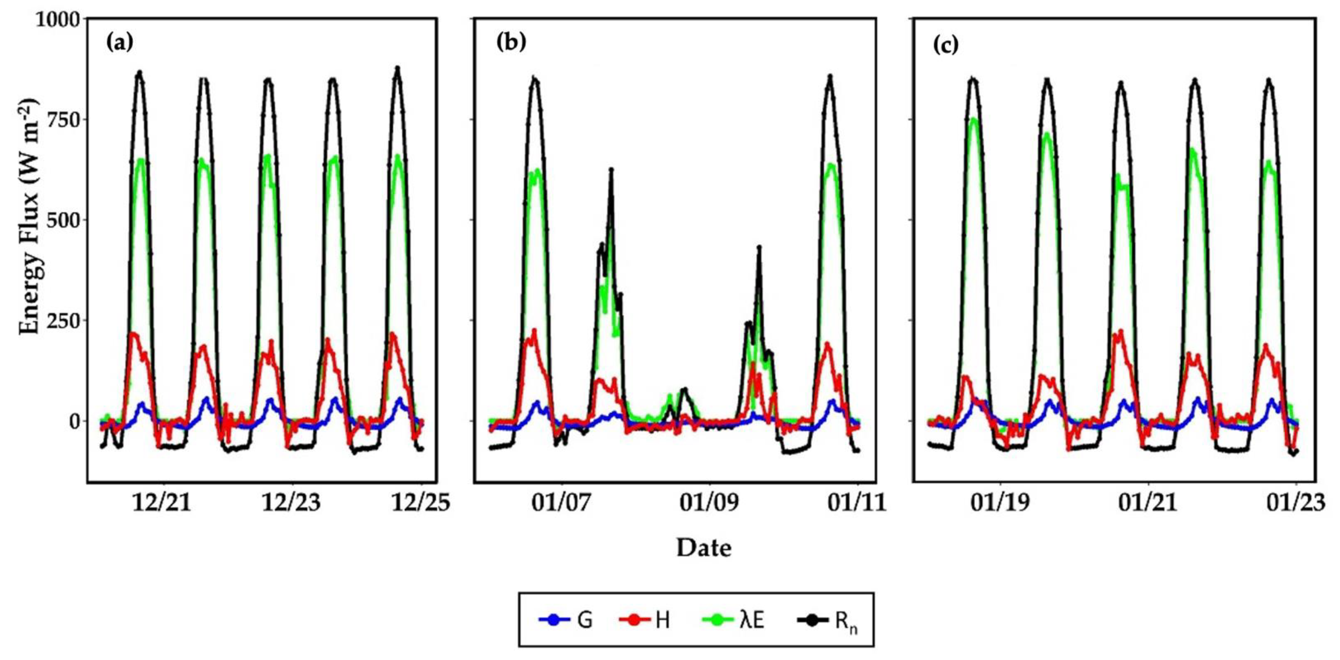
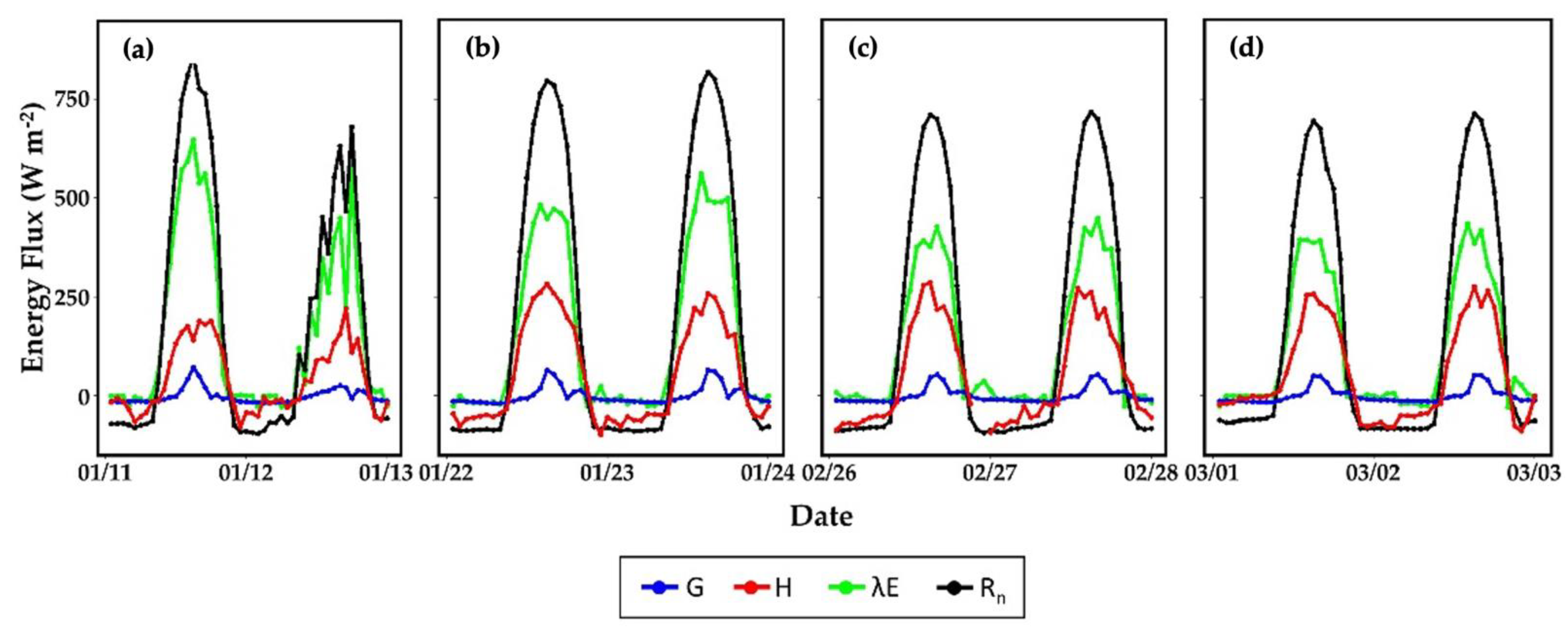
3.1.1. Surface Energy Balance Measurements during Calibration

The hourly values of the SEB parameters during each field campaign at sites S1 and S2 are shown in Figure 5 and Figure 6, respectively. RH was 10–30% lower, and Ta, u, and VPD were 10–15%, 10–20%, and 10–30% higher, respectively, in mid-January than during other dates at both sites.
At site S1, daily averages of the H/Rn fraction were 0.21, 0.21, and 0.18 during the first, second, and third field campaigns, respectively. H/Rn was frequently lower during the first 2 days after irrigation, while λE was similar at 3 days after irrigation across field campaigns. Most of the Rn was converted into λE, while H was often small (i.e., 15–40% of Rn) in well-irrigated crop systems (Figure 5). Mean daily Rn was positive during the summer at the site and reached a maximum of nearly 850 W m−2 on clear, sunny days and 150–450 W m−2 on cloudy days (Figure 5b). G was the smallest energy component of the SEB (0.5–1.5% of Rn) and as low as 3.0 W m−2 due to cloudy days during the second field campaign. Conditions during the second field campaign also resulted in lower λE. At that point, average Ta decreased by 15%, and average u increased by 20% relative to the other measurement periods. In contrast, λE was highest, on average, during the third field campaign due to warm, sunny weather and greater phenological development in the hazelnut trees.
At site S2, daily averages of the H/Rn fraction were 0.22, 0.25, 0.30, and 0.32 during the first, second, third, and fourth field campaigns, respectively. H/Rn was similar between campaigns because the trees were irrigated every 2 days, and H was often small compared to λE in well-irrigated cropping systems (Figure 6). Maximum daily Rn was nearly 800 W m−2 on a clear day in January (Figure 6b), 715 W m−2 on clear days in February (Figure 6c) and March (Figure 6d), and ≈650 W m−2 on a cloudy day in January (Figure 6a). During each campaign, daily G hovered mostly near zero, and λE was lowest during day 2 of the first campaign due to heavy cloud cover. λE also decreased slightly when the trees were closer to harvest in February and March.
In general, the SEB measurements differed between the sites, which could be attributed to the irrigation method. Determining the water requirements of orchards irrigated by drip and micro-sprinklers requires good knowledge of H/Rn, G/Rn, and λE/Rn ratios, which depend on tree vigor, soil water, and energy availability. Vigor is manifested mainly through canopy size and density, LAI, and P [45]. Lopez et al. [46] suggested that these parameters, along with pruning and the irrigation system, have a significant effect on the partitioning of Rn. Depending on soil water availability, the canopy structure, and P, the amount of H generated at the soil surface can be a major contributor to the energy balance [46], similar to what was observed at site S2. Ortega et al. [45] found similar results in an olive orchard.
The previous SEB measurements at sites S1 and S2 were used to calibrate the SEB-PW model. The calibration results are shown in Table 2. Once the model was calibrated, it was evaluated using the data measured during three growing seasons.

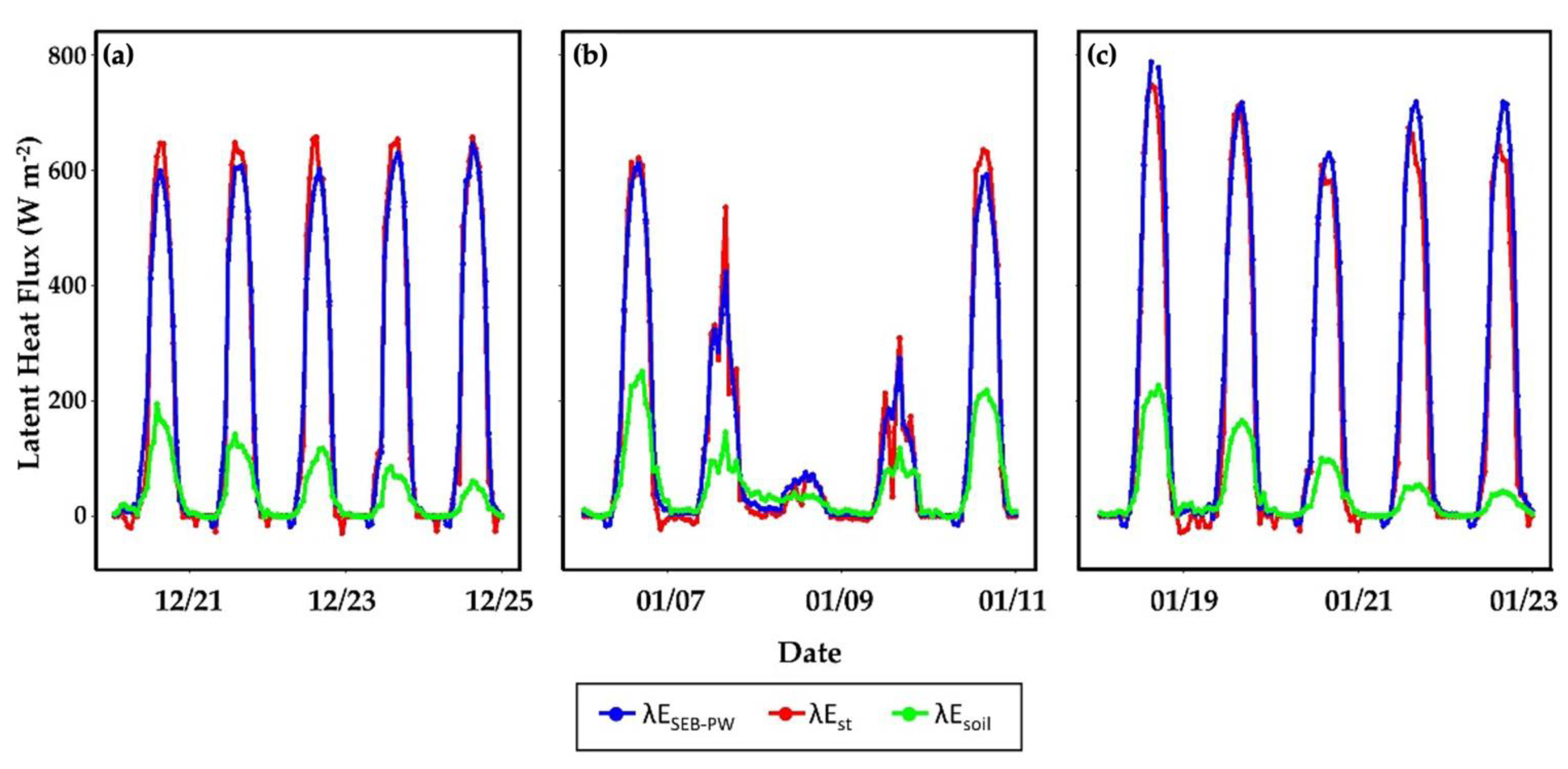
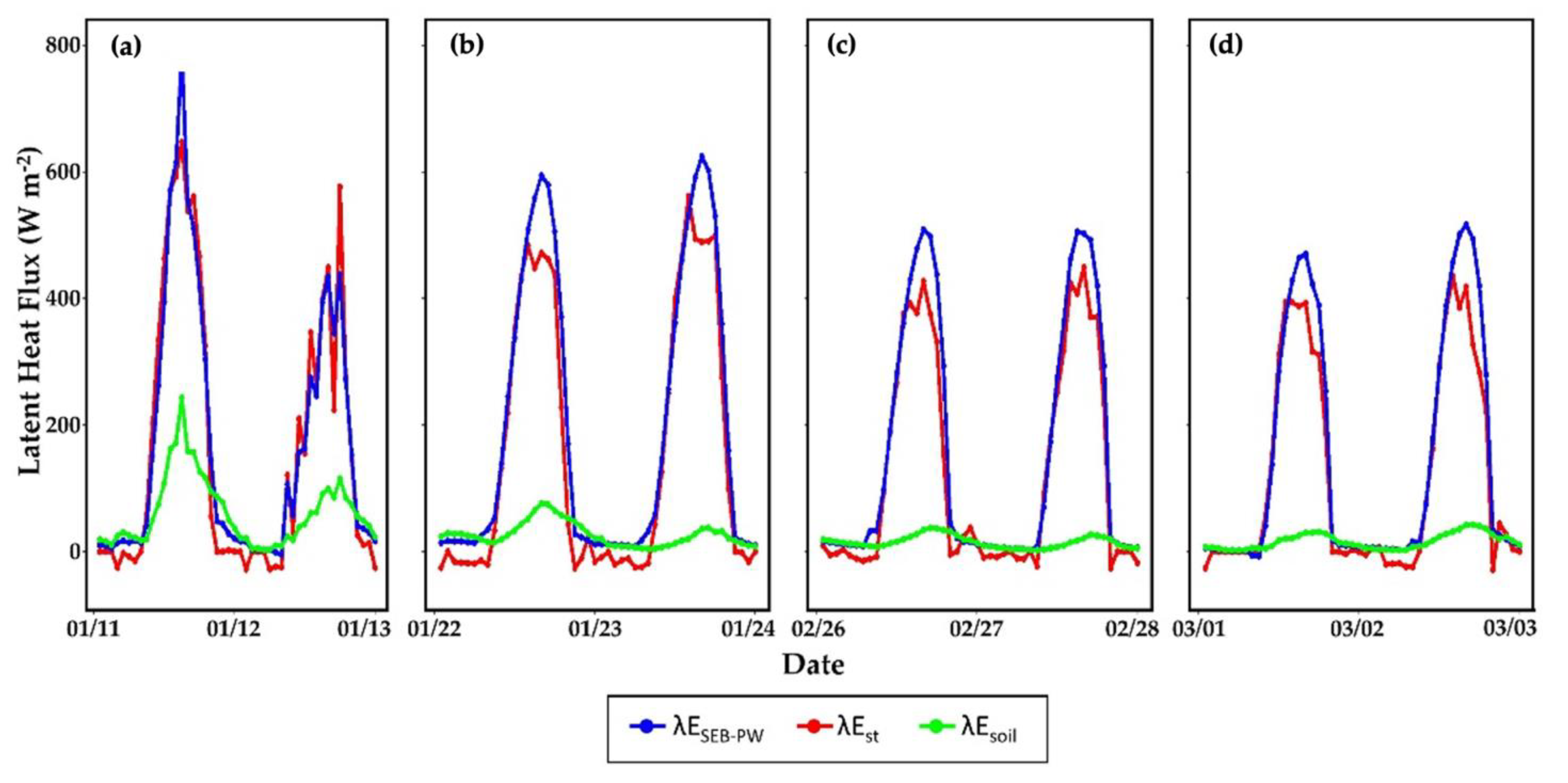
3.1.2. Diurnal Dynamics of ET and E after Calibration

The hourly values estimated with the SEB-PW model and λE measured using the ET station during all field campaigns at sites S1 and S2 are presented in Figure 7 and Figure 8, respectively.
At site S1, the diurnal dynamics of λE estimated with the SEB-PW model were similar to the values measured with the ET station (Figure 7). During the 2018–2019 growing season, λE flux reached a maximum at midday of 715 W m−2 on January 18, which was a clear and sunny day. In contrast, values were much lower on January 7 (480 W m−2), 8 (67 W m−2), and 9 (300 W m−2) due to clouds and rain. Overall, ET estimates with the SEB-PW model were 2% to 8% less than the measured values. As was expected, latent heat flux from the soil (λEsoil) was higher on the first day after irrigation and decreased during the following days, except during the second field campaign (Figure 7b).
At site S2, the diurnal dynamics of λE estimated with the SEB-PW model and measured with the ET station at site S2 were similar to those at site S1. At this site, λE flux reached a maximum of 670 W m−2 on 11 January (sunny) and a minimum of 500 W m−2 on 12 January (cloudy). ET values estimated with the SEB-PW model were slightly higher than the values measured with the ET station, mainly between the hours of 13:00 and 15:00. λEsoil was lower at site S2 than at site S1 due to a smaller wetted soil fraction with drip (S2) than with micro-sprinklers (S1).
Since micro-sprinklers generated higher Pw than the drip irrigation system, E was generally higher at site S1 than at S2 (Figure 7 and Figure 8). However, as a canopy grows, it increasingly covers the more wetted area and, therefore, reduces the amount of radiation reaching the soil and, consequently, the energy available for E from the wetted area [47].

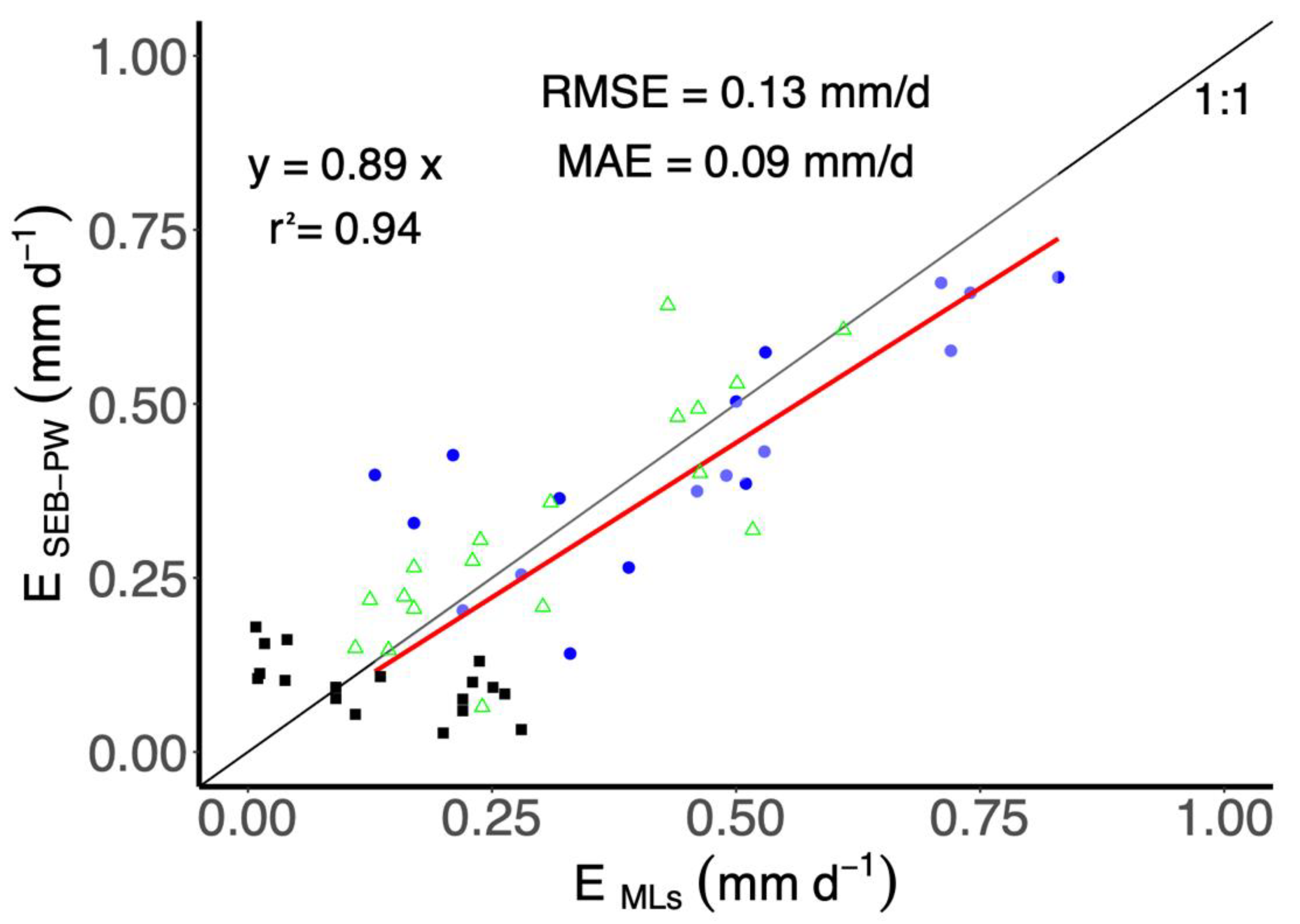
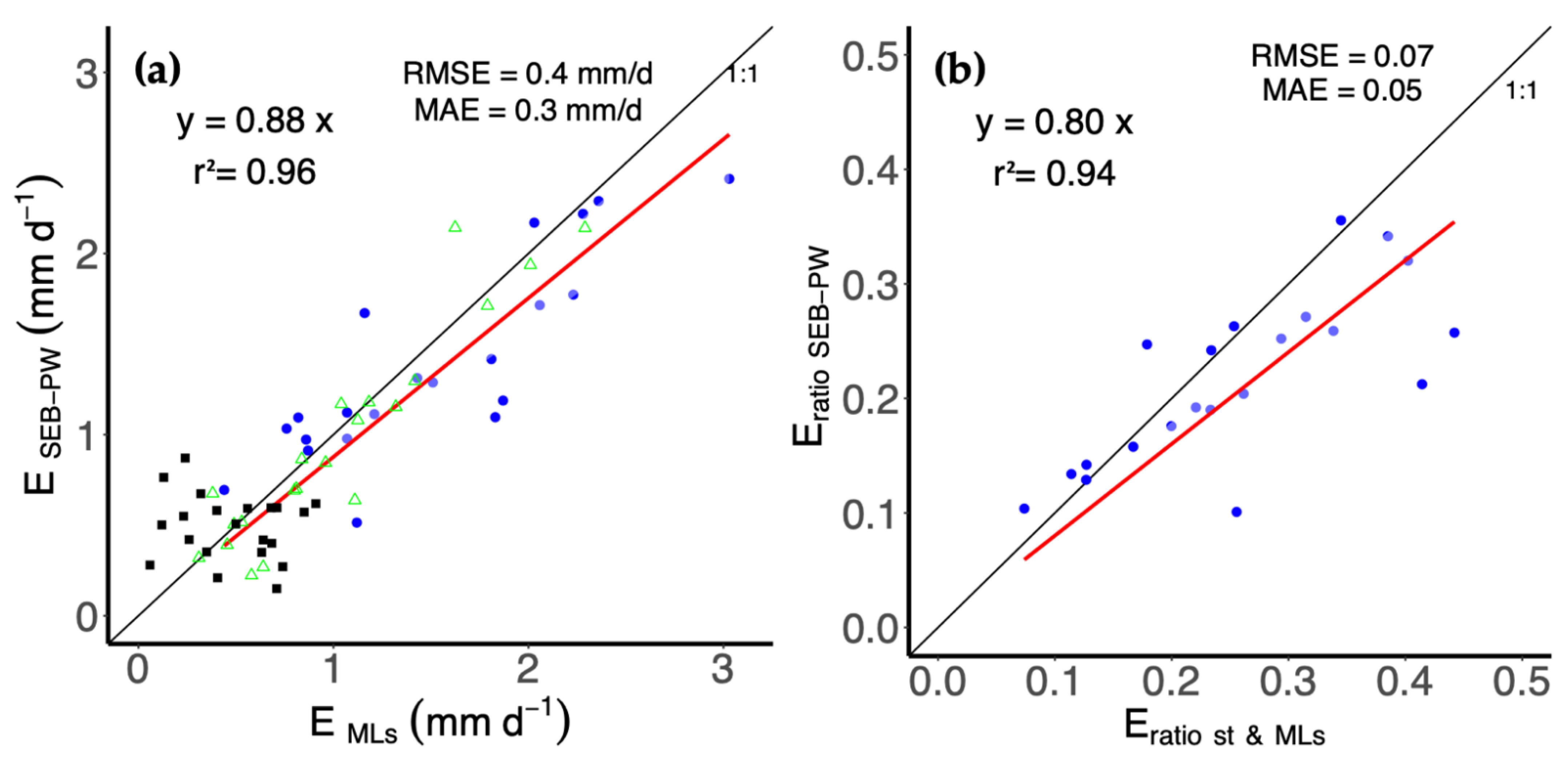
3.1.3. Comparison of Diurnal, Nightly, and Daily Soil E

Diurnal E estimated by the SEB-PW model versus values measured with ET stations and micro-lysimeters are shown in Figure 9a. Average E decreased from 2.3 mm d−1 during the first day after irrigation to 0.8 mm d−1 during the following days. Patterns of increasing and decreasing E are consistent with the effect of irrigation frequency at both sites. A substantial decrease in E was observed at site S1, which had longer irrigation intervals (6 days), as well as a larger wetted area, than site S1. Diurnal E measurements and SEB-PW predictions on all days at sites S1 and S2 exhibit a similar distribution around the 1:1 line (Figure 9a). The SEB-PW model presented an r2 of 0.87 and a slope of 1.0. Furthermore, when compared to field measurements, diurnal E estimates from the SEB-PW model resulted in an RMSE of 0.5 mm d−1, an MAE of 0.4 mm d−1, an NSE of 0.62, and a da of 0.85.
With one exception, the measured evaporation ratio (Eratio), calculated as the ratio between total soil E and total ET, was higher the first day after irrigation, with values ranging between 25% and 34% at site S1 and between 22% and 28% at site S2 (Figure 9b). Jara et al. [48] found that daily E measured with MLs accounted for 14% of total ET during 28 days of observation in corn (Zea Mays L.), which is lower than observed in the present study because corn fields have higher planting densities than hazelnut orchards. Montoro et al. [18] found similar values of E in grapevines, i.e., 11% to 31% of total ET. When compared to field measurements, RMSE and MAE of the diurnal Eratio estimated by the SEB-PW model were 0.08 and 0.07, respectively. Diurnal E from non-wetted areas (black squares, Figure 9a) was 30% and 37% of total diurnal E measured with MLs at site S1 and S2, respectively, while diurnal E from wetted areas was 70% and 63%, respectively (green triangles, Figure 9a). At both sites, diurnal E estimated from the SEB-PW model were similar to diurnal E measured by MLs in wetted and non-wetted areas.
Nightly E estimated by the SEB-PW model versus the values measured with MLs is shown in Figure 10. Nightly E estimated by the model presented an r2 of 0.94, with a regression slope of 0.89. For nightly E, MAE was 0.09 mm d−1, while RMSE was 0.13 mm d−1, NSE was 0.60, and da was 0.90. It was observed that nightly E was similar between the orchards with micro-sprinkler and drip irrigation systems and averaged 0.45 mm d−1 at both sites. In both cases, nightly E ranged between 5% to 10% of total ET. Jara et al. [48] found lower nightly E values in a corn field, with an average of 0.2 mm per night, accounting for only 5.5% of total ET. Meanwhile, Colaizzi et al. [49] measured nightly E values between 0.01 to 0.34 mm in a cotton field irrigated by a lateral-moving sprinkler system.
Daily E measurements and SEB-PW predictions for both sites S1 and S2 exhibited a deviation from the 1:1 line (Figure 11a). Daily E estimations by the SEB-PW model presented an underestimation with respect to the E measured with MLs (r2 of 0.96 and regression slope of 0.88). The daily weighted average of E estimated by the model for micro-sprinkler (site S1) and drip (site S2) irrigation systems were 1.5 and 1.1 mm d−1, at site S1 and S2, respectively, while those measured with MLs were 1.6 and 1.4 mm d−1, respectively. The maximum daily E value measured with MLs was 3.0 ± 0.05 mm d−1 with the micro-sprinklers and 2.1 ± 0.04 mm d−1 with the drip system and, in both cases, was observed a day after irrigation was applied. Furthermore, daily E was lower (approximately 0.4 mm d−1) each day before irrigation compared to 2 or 3 days after irrigation. When compared to field measurements, daily E estimates from the SEB-PW model resulted in an RMSE of 0.4 mm d−1, an MAE of 0.3 mm d−1, an NSE of 0.69, and a da of 0.88.
As with diurnal E, measured Eratio was higher the first day after irrigation, with values ranging between 34% and 39% of total ET at site S1 and 29% and 42% of total ET at site S2 (Figure 11b). The modeled Eratio was also higher on the first day after irrigation at both sites, with values ranging between 27% and 32% of total ET at site S1 and 26% and 34% of total ET at S2. Meanwhile, lower Eratio values were measured on the second day after irrigation at site S2 and the fifth day after irrigation at site S1, averaging 18% and 13%, respectively. Similar values were simulated by the SEB-PW model. Daily E from non-wetted areas measured with MLs (black squares, Figure 11a) was 32% of total daily E at site S1 and 35% of total daily E at site S2, similar to values found by the SEB-PW model. Daily E from wetted areas (green triangles, Figure 11a) was 68% of the total diurnal E at site S1 and 65% at site S2. Similar Eratio values were reported in the literature when measured daily Eratio values were compared to predictions from energy balance models [18,21,48,49]. Based on the statistical parameters (Table 3), the calibrated SEB-PW model showed good agreement between measured and calculated daily E (24 h).

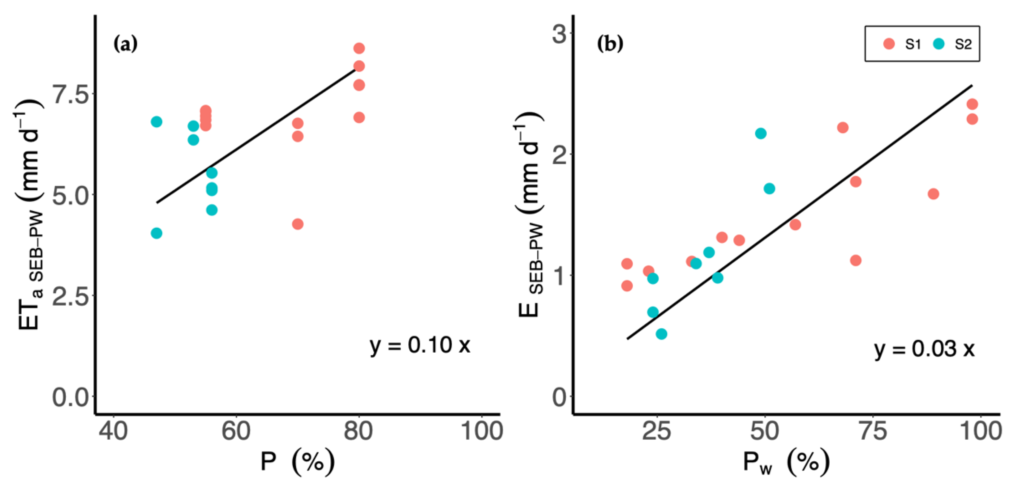
3.2. E and Actual ET Comparison for Micro-Sprinkler and Drip Irrigation Systems

The daily actual ET (ETa) and E modeled by the SEB-PW model at sites S1 (micro-sprinkler irrigation) and S2 (drip irrigation) were analyzed to compare the differences between the two irrigation systems (Figure 12a,b). ETa modeled at site S1 was, in general, higher compared to site S2 due to the irrigation method associated with the wetted area and the canopy cover. The P measured at site S1 was higher than at site S2; therefore, intercepted solar radiation was also higher, leading to an increase in ETa. Fereres et al. [50] first studied the relationship between ETa and P and found a nearly linear relationship between the percentage of the estimated ET of a mature almond orchard and the area shaded by the trees. Other researchers, e.g., Marino et al. [51] and Marsal et al. [52], discovered a direct relationship between cumulative ET and PAR (photosynthetically active radiation) light interception by the tree canopy and found that the higher the PAR light interception by the tree canopy, the higher ET. For all data and field campaigns at both sites, ETa presented an r2 of 0.97 concerning P and was similar to values in the literature [50,51] (Figure 12). Testi et al. [47] deduced that the increase in ET induced by the wet area depends on the Pw by the micro-irrigation system.
E modeled by the SEB-PW model versus the Pw is shown in Figure 12b. The micro-irrigation systems (i.e., drip and micro-sprinkler) only wet a fraction of the total soil volume. The soil area wetted by a micro-sprinkler irrigation system is, in theory, larger than that of a drip irrigation system; therefore, potential decreases in ET under a drip irrigation system are associated with a decrease in the E (Figure 12b). The average E at S1 was 30% higher than at S2. At site S1, the highest E occurred when Pw was near 95%, with values close to 2.5 mm d−1. For S2, this occurred when Pw was approximately 50%, with E values close to 1.8 mm d−1 and 2.1 mm d−1. A direct relationship between E and Pw was observed, presenting an r2 of 0.93 (Figure 12b).

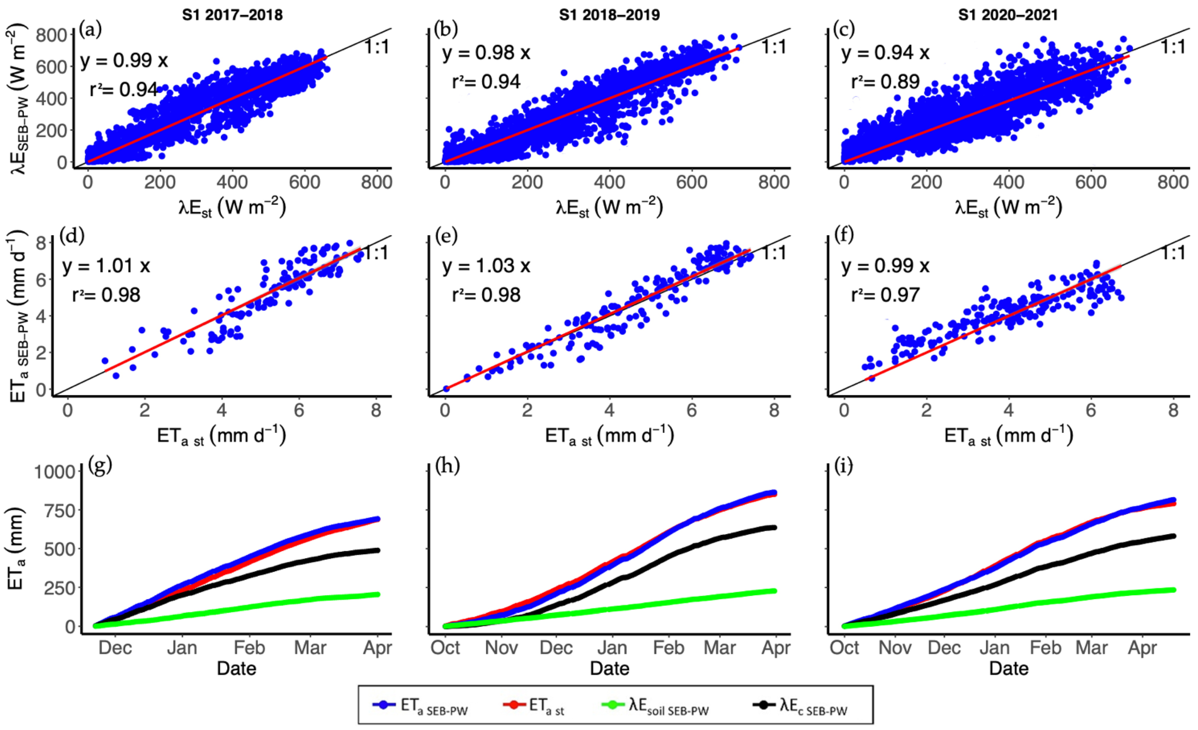
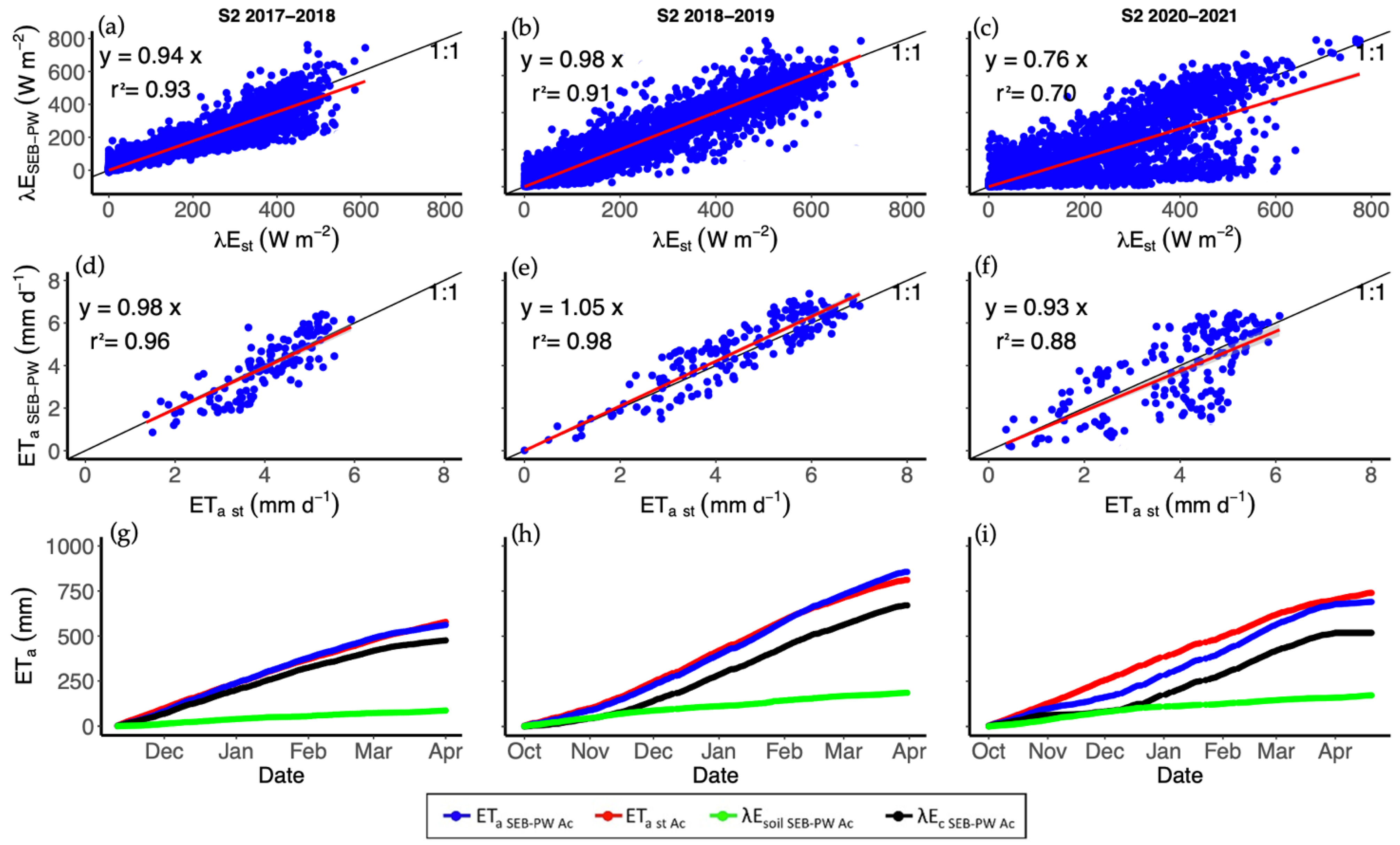
3.3. Model Validation: Seasonal Dynamics of E, Crop T, and ET

The hourly measurements and SEB-PW predictions were analyzed to evaluate the model performance for each growing season at sites S1 (Figure 13) and S2 (Figure 14). Daily measurements and predictions are shown in Figure 13d–f (site S1) and Figure 14d–f (site S2), and cumulative actual ET (ETast), ET (ETa SEB-PW), soil E (λEsoil SEB-PW), and crop T (λEc SEB-PW) are shown in Figure 13g–i (site S1) and Figure 14g–i (site S2).
At site S1, each growing season, λE measured with the ET station was highly correlated to the values calculated by the SEB-PW model (Table 4). Similar results have been reported in other studies when the measured hourly dynamics of λE are compared to predictions from energy balance models [32,36,53,54]. In the present study, the difference in Etast and Etast SEB-PW between the first and latter two growing seasons was mainly due to the start date of the data collection, which was initiated on 20 November during 2017–2018 and October 1 during 2018–2019 and 2020–2021. The ratio of annual ET calculated with the SEB-PW model to the annual ET measured with the ET station was between 0.97 and 1.07, while cumulative E values from the model were 24% to 28% of cumulative ET. Crop T estimated by the model was 72% to 76% of the annual ET.
At site S2, similar to site S1, λE measured with the ET station was highly correlated to the values calculated by the SEB-PW model at site S2 (Table 4). Whether it was measured or modeled, cumulative ET, in this case, was lower than at site S1 and ranged between 600 mm to 780 mm (Table 5). Once again, a difference in ETast and ETast SEB-PW between the first and latter two growing seasons was mainly due to the start date of the data collection, which was initiated on 10 November during 2017–2018 and October 1 during 2018–2019 and 2020–2021. The ratio of annual ET calculated with the SEB-PW model to the annual ET measured with the ET station was between 0.98 and 1.01, while cumulative E values from the model were 15% to 19% of cumulative ET. Crop T estimated by the model was 83% to 85% of the annual ET.
When the entire surface of the orchard was wetted, the total ET mostly consisted of E. This typically occurs after a rainy day or during the winter. During the growing season, E decreased markedly, while crop T became the largest component of total ET (Figure 13g–i and Figure 14g–i). A comparison of cumulative E between the sites illustrates the level by which the micro-sprinklers increased E relative to drip irrigation (less wetted area). Testi et al. [47] indicated that the combined effects of micro-advection, aerodynamic sheltering, and intermittent shading make a mechanistic model of ET and E from wetted and non-wetted areas difficult to develop; however, the presented SEB-PW model produced good results based on statistical parameters (Table 5).
The results show that ET estimated from the SEB-PW model was in good agreement with the ET measurements in both hazelnut orchards. These results are significant because they provide a better understanding of soil E when using different micro-irrigation systems and allow the user to divide crop water consumption into separate components, including crop T, soil E, and total ET. The model improved estimates of soil E by allowing wetted and non-wetted areas to be calculated separately. According to the statistical results obtained, RMSE, MAE, NSE, and da were in agreement with one another and corroborated that the SEB-PW model provides accurate estimates of both ET and E.

4. Conclusions

The SEB-PW model was evaluated using Rn, H, G, and E measurements obtained in two hazelnut orchards with different P and Pw irrigated by micro-sprinkler and drip irrigation systems during three growing seasons. Measurements of Rn, H, and G were obtained by an ET station at each study site, and λE was determined with the SEB method that calculates λE as the residual from Rn, G, and H, while E was obtained with MLs installed in non-wetted and wetted areas. In addition, there was an hourly agreement between estimated and measured λE for the three growing seasons at both sites, da varied between 0.85 and 0.98, NSE between 0.70 and 0.92, MAE between 29.4 W m−2 and 55.8 W m−2, and RMSE between 48.6 W m−2 to 95.1 W m−2. Soil E calculated with the SEB-PW model and E measured with MLs had an r2 of 0.87 to 0.94 for diurnal E and nightly E analysis, while better results were obtained for daily E, with an r2 of 0.96. E from non-wetted areas was 29% of total E, while E from wetted areas accounted for the remaining 71%. Average nightly E was between 5 and 10% of daily E. Cumulative E from the SEB-PW model for all three growing seasons was 24% to 28% of cumulative ET for micro-sprinkler irrigation (site S1) and 15% to 19% for drip irrigation (site S2). Likewise, crop T estimated by the SEB-PW model was 72% to 76% of the annual ET at site S1 and 81% to 85% of the annual ET at site S2. The results show that ET estimates from the SEB-PW model were in good agreement with the ET measurements in both hazelnut orchards. With the SEB-PW model, it is possible to partition total crop ET into crop T and soil E. Specifically, the SEB-PW model may be used to calculate soil E from wetted and non-wetted areas separately. This research is expected to have future implications for irrigation system decision-making, design, and management, which considering the benefits of the results obtained for estimating diurnal and seasonal soil E, could save water and aid local and regional water conservation.

Author Contributions

Conceptualization: C.S., O.L. and E.H.; Data curation: C.S.; Formal analysis: C.S.; Investigation: C.S., O.L. and E.H.; Funding acquisition: C.S. and G.V.; Methodology: C.S., O.L. and E.H.; Supervision: O.L.; Validation: C.S.; Visualization: C.S. and C.R.; Writing—original draft: C.S.; Writing—review and editing: C.S., O.L., E.H., C.R., D.R.B. and G.V. All authors have read and agreed to the published version of the manuscript.

Funding

The research leading to this report was supported by the National Research and Development Agency (ANID) through CONICYT-PCHA/Doctorado Nacional/2015-21150829, the ANID/FONDAP/15130015 project: Water Research Center for Agriculture and Mining (CRHIAM), and supported by the University of Concepción through the VRID No.2021000217INI project.

Institutional Review Board Statement

Not applicable.

Informed Consent Statement

Not applicable.

Data Availability Statement

Not applicable.

Acknowledgments

The authors thank the ANID/FONDAP/15130015 project: Water Research Center for Agriculture and Mining (CRHIAM), ANID/Becas Chile/Postdoctorado en el extranjero 2022/74220053, CONICYT-PCHA/Doctorado Nacional/2015-21150829, the VRID No.2021000217INI project, and the Department of Water Resources at the Universidad de Concepción. We gratefully acknowledge Carlos Cea for helping with the field measurements.

Conflicts of Interest

The authors declare no conflict of interest.

Appendix A. Summary of the SEB-PW Model

The SEB-PW model distributes net radiation (Rn) into latent and sensible heat ( λ E and H), as well as soil heat (G) fluxes through the soil–canopy system, according to the energy balance:
Rn λ E H G = 0 ,
H = H c + H bs + H s ,
λ E = λ E c + λ E bs + λ E s ,
where H c , H bs , and H s are the sensible heat from the canopy, bare soil, and soil shaded below the canopy (W m−2), respectively, and λ Ec, λ Ebs, and λ Es are the latent heat from the canopy, the bare soil between rows, and the soil below the canopy soil (W m−2), respectively. Physical and chemical energy storage terms in the canopy–soil system are not considered.
Considering the wet soil fraction (Pw), the latent heat flux from the bare soil between the rows and soil under the canopy becomes:
λ E s = λ E ss · ( 1 P w ) + λ E sh · ( P w ) ,
λ E bs = λ E bss · ( 1 P w ) + λ E bsh · ( P w ) ,
where P w is the wet soil fraction (0 < Pw < 1), λ Ess and λ Esh are the soil evaporation under the canopy for non-wetted and wetted areas (W m−2 and W m−2), respectively, and λ Ebss and λ Ebsh are the soil evaporation for the bare soil between the rows under non-wetted and wetted conditions (W m−2 and W m−2).
Including the differences in vapor pressure and temperature between levels (reference height, canopy, top soil, and lower soil layer), the latent heat fluxes from the canopy, under the canopy, and bare soil are estimated as:
λ E c = R nc · Δ · r 1 + ρ · C P · ( e b * e b ) γ · ( r 1 + r c ) + Δ · r 1 ,
λ E s = R nDC · Δ · r L · r 2 + ρ · C P · ( e b * e b ) · ( r us + r uh + r L + r 2 ) ρ · C P · Δ · ( T b T m ) · ( r us + r uh + r 2 ) γ · r A · ( r us + r uh + r L + r 2 ) + Δ · r L · ( r us + r uh + r 2 ) ,
λ E bs = R ne · Δ · r 2 L · r 2 b + ρ · C P · ( e b * e b ) · ( r 2 u s + r 2 u h + r 2 L + r 2 b ) ρ · C P · Δ · ( T b T m ) · ( r 2 u s + r 2 u h + r 2 b ) γ · r B · ( r 2 u s + r 2 u h + r 2 L + r 2 b ) + Δ · r 2 L · ( r 2 u s + r 2 u h + r 2 b ) ,
where Rnc, RnDC, and Rne are the net radiation absorbed by the canopy, below the canopy, and absorbed by the soil between rows (W m−2), respectively; ρ is the density of moist air (1.013 kg m−3); Cp is the specific heat of air (1013 J kg−1 °C−1); γ is the psychrometric constant (kPa °C−1); e b is the vapor pressure of the atmosphere at the canopy level (kPa); r 1 is aerodynamic resistance between the canopy and the air (s m−1); r c is the surface canopy resistance (s m−1); r L and r 2 L are the soil heat flux resistance for the lower layer under the canopy area and from the bare soil (s m−1), respectively; r 2 is the aerodynamic resistance between the canopy and the air at the canopy level (s m−1); r u s , r u h , r 2 u s , and r 2 u h are the soil heat flux resistance under the canopy and bare soil for the non-irrigated and irrigated upper layer (s m−1), respectively; T m is the soil temperature at the bottom of the lower layer (°C); r 2 b is the aerodynamic resistance between the air around the bare soil and the canopy height and the bare soil level (s m−1). See Souto et al. [14] for the other surface energy balance components and further details.

References

  1. Food and Agriculture Organization of the United Nations. FAOSTAT. Available online: https://www.fao.org/faostat/en/#data/QCL (accessed on 22 May 2019).
  2. Valentini, N.; Moraglio, S.T.; Rolle, L.; Tavella, L.; Botta, R. Nut and Kernel Growth and Shell Hardening in Eighteen Hazelnut Cultivars (Corylus avellana L.). Hortic. Sci. 2015, 42, 149–158. [Google Scholar] [CrossRef] [Green Version]
  3. Fideghelli, C.; De Salvador, F.R. World Hazelnut Situation and Perspectives. Vii Int. Congr. Hazelnut 2009, 845, 39–51. [Google Scholar] [CrossRef]
  4. ODEPA Ficha Nacional. Available online: https://bibliotecadigital.odepa.gob.cl/bitstream/handle/20.500.12650/69897/FichaNacional2022.pdf (accessed on 18 May 2022).
  5. Revista MundoAgro. Gigante En Camino: “El 1° Día Internacional Del Avellano Europeo”. Available online: http://www.mundoagro.cl/revistas/numero-113-abril-2019/ (accessed on 24 May 2019).
  6. Bignami, C.; Cristofori, V.; Bertazza, G. Effects of Water Availability on Hazelnut Yield and Seed Composition during Fruit Growth. Acta Hortic. 2011, 922, 333–340. [Google Scholar] [CrossRef]
  7. Cristofori, V.; Muleo, R.; Bignami, C.; Rugini, E. Long Term Evaluation of Hazelnut Response to Drip Irrigation. Acta Hortic. 2014, 1052, 179–186. [Google Scholar] [CrossRef]
  8. Bignami, C.; Cammilli, C.; Moretti, G.; Romoli, F. Irrigation of Corylus avellana L.: Effects on Canopy Development and Production of Young Plants. Acta Hortic. 2000, 537, 903–910. [Google Scholar] [CrossRef]
  9. Dias, R.; Gonçalves, B.; Moutinho-Pereira, J.; Carvalho, J.L.; Silva, A.P. Effect of Irrigation on Physiological and Biochemical Traits of Hazelnuts (Corylus avellana L.). Acta Hortic. 2005, 686, 201–206. [Google Scholar] [CrossRef]
  10. Bignami, C.; Natali, S. Influence of Irrigation on the Growth and Production of Young Hazelnuts. Acta Hortic. 1997, 445, 247–251. [Google Scholar] [CrossRef]
  11. Tombesi, A. Influence of Soil Water Levels on Assimilation and Water Use Efficiency in Hazelnuts. Acta Hortic. 1994, 351, 247–255. [Google Scholar] [CrossRef]
  12. Tindula, G.N.; Orang, M.N.; Snyder, R.L. Survey of Irrigation Methods in California in 2010. J. Irrig. Drain. Eng. 2013, 139, 233–238. [Google Scholar] [CrossRef]
  13. Burt, C.M.; Howes, D.J.; Mutziger, A. Evaporation Estimates for Irrigated Agriculture in California. In Proceedings of the 2001 Irrigation Association Conference, San Antonio, TX, USA, 4–6 November 2001. [Google Scholar]
  14. Souto, C.; Lagos, O.; Holzapfel, E.; Maskey, M.L.; Wunderlich, L.; Shapiro, K.; Marino, G.; Snyder, R.; Zaccaria, D. A Modified Surface Energy Balance to Estimate Crop Transpiration and Soil Evaporation in Micro-Irrigated Orchards. Water 2019, 11, 1747. [Google Scholar] [CrossRef]
  15. Burt, C.M.; Mutziger, A.J.; Allen, R.G.; Howell, T.A. Evaporation Research: Review and Interpretation. J. Irrig. Drain. Eng. 2005, 131, 37–58. [Google Scholar] [CrossRef] [Green Version]
  16. Idso, S.B.; Reginato, R.J.; Jackson, R.D.; Kimball, B.A.; Nakayama, F.S. The Three Stages of Drying of a Field Soil. Soil Sci. Soc. Am. J. 1974, 38, 831–837. [Google Scholar] [CrossRef]
  17. Deol, P.; Heitman, J.; Amoozegar, A.; Ren, T.; Horton, R. Quantifying Nonisothermal Subsurface Soil Water Evaporation. Water Resour. Res. 2012, 48, 1–11. [Google Scholar] [CrossRef] [Green Version]
  18. Montoro, A.; Ma, F. Transpiration and Evaporation of Grapevine, Two Components Related to Irrigation Strategy. Agric. Water Manag. 2016, 177, 193–200. [Google Scholar] [CrossRef]
  19. Fandiño, M.; Cancela, J.J.; Rey, B.J.; Martínez, E.M.; Rosa, R.G.; Pereira, L.S. Using the Dual-Kc Approach to Model Evapotranspiration of Albariño with Consideration of Active Ground Cover (Vitis vinifera L. Cv. Albariño) with Consideration of Active Ground Cover. Agric. Water Manag. 2012, 112, 75–87. [Google Scholar] [CrossRef]
  20. Cancela, J.J.; Fandiño, M.; Rey, B.J.; Martínez, E.M. Automatic Irrigation System Based on Dual Crop Coefficient, Soil and Plant Water Status for Vitis vinifera (Cv Godello and Cv Mencía). Agric. Water Manag. 2015, 151, 52–63. [Google Scholar] [CrossRef]
  21. Paço, T.A.; Paredes, P.; Pereira, L.S.; Silvestre, J.; Santos, F.L. Crop Coefficients and Transpiration of a Super Intensive Arbequina Olive Orchard Using the Dual K c Approach and the K Cb Computation with the Fraction of Ground Cover and Height. Water 2019, 2, 383. [Google Scholar] [CrossRef] [Green Version]
  22. Bignami, C.; Cristofori, V.; Ghini, P.; Rugini, E. Effects of Irrigation on Growth and Yield Components of Hazelnut (Corylus avellana L.) in Central Italy. Acta Hortic. 2009, 845, 309–314. [Google Scholar] [CrossRef]
  23. Ortega-Farías, S.; Villalobos-Soublett, E.; Riveros-Burgos, C.; Zúñiga, M.; Ahumada-Orellana, L.E. Effect of Irrigation Cut-off Strategies on Yield, Water Productivity and Gas Exchange in a Drip-Irrigated Hazelnut (Corylus avellana L. Cv. Tonda Di Giffoni) Orchard under Semiarid Conditions. Agric. Water Manag. 2020, 238, 106173. [Google Scholar] [CrossRef]
  24. Allen, R.G.; Pereira, L.S.; Raes, D.; Smith, M. Crop Evapotranspiration-Guidelines for Computing Crop Water Requirements; FAO Irrigation and Drainage Paper 56; FAO: Rome, Italy, 1998; Volume 300, p. D05109. [Google Scholar]
  25. Allen, R.G.; Tasumi, M.; Trezza, R. Satellite-Based Energy Balance for Mapping Evapotranspiration with Internalized Calibration (METRIC)—Model. J. Irrig. Drain. Eng. 2007, 133, 380–394. [Google Scholar] [CrossRef]
  26. Shuttleworth, W.J.; Wallace, J.S. Evaporation from Sparse Crops-an Energy Combination Theory. Q. J. R. Meteorol. Soc. 1985, 111, 839–855. [Google Scholar] [CrossRef]
  27. Choudhury, B.J.; Monteith, J.L. A Four-Layer Model for the Heat Budget of Homogeneous Land Surfaces. Q. J. R. Meteorol. Soc. 1988, 114, 373–398. [Google Scholar] [CrossRef]
  28. Shuttleworth, W.J. Towards One-Step Estimation of Crop Water Requirements. Trans. ASABE 2006, 49, 925–935. [Google Scholar] [CrossRef]
  29. Octavio, L.; Derrel, L. Surface Energy Balance Model of Transpiration from Variable Canopy Cover and Evaporation from Residue-Covered or Bare Soil Systems: Model Evaluation. Irrig. Sci. 2013, 31, 135–150. [Google Scholar] [CrossRef] [Green Version]
  30. Lagos, L.O.; Merino, G.; Martin, D.; Verma, S.; Suyker, A. Evapotranspiration of Partially Vegetated Surfaces. In Evapotranspiration-Remote Sensing and Modeling; InTech: London, UK, 2012. [Google Scholar]
  31. Fuentes-Peñailillo, F.; Ortega-Farías, S.; Acevedo-Opazo, C.; Fonseca-Luengo, D. Implementation of a Two-Source Model for Estimating the Spatial Variability of Olive Evapotranspiration Using Satellite Images and Ground-Based Climate Data. Water 2018, 10, 339. [Google Scholar] [CrossRef] [Green Version]
  32. Ortega-Farías, S.; Carrasco, M.; Olioso, A.; Acevedo, C.; Poblete, C. Latent Heat Flux over Cabernet Sauvignon Vineyard Using the Shuttleworth and Wallace Model. Irrig. Sci. 2007, 25, 161–170. [Google Scholar] [CrossRef]
  33. Farahani, H.J.; Ahuja, L.R. Evapotranspiration Modeling of Partial Canopy/Residue-Covered Fields. Trans. ASAE 1996, 39, 2051–2064. [Google Scholar] [CrossRef]
  34. Iritz, Z.; Lindroth, A.; Heikinheimo, M.; Grelle, A.; Kellner, E. Test of a Modified Shuttleworth-Wallace Estimate of Boreal Forest Evaporation. Agric. For. Meteorol. 1999, 98, 605–619. [Google Scholar] [CrossRef]
  35. Colaizzi, P.D.; Agam, N.; Tolk, J.A.; Evett, S.R.; Howell, T.A.; Gowda, P.H.; Kustas, W.P.; Anderson, M.C. Two-Source Energy Balance Model to Calculate E, T, and ET: Comparison of Priestley-Taylor and Penman-Monteith Formulations and Two Time Scaling Methods. Trans. ASABE 2014, 57, 479–498. [Google Scholar] [CrossRef] [Green Version]
  36. Odhiambo, L.O.; Irmak, S. Performance of Extended Shuttleworth-Wallace Model for Estimating and Partitioning of Evapotranspiration in a Partial Residue-Covered Subsurface Drip-Irrigated Soybean Field. Trans. ASABE 2011, 54, 915–930. [Google Scholar] [CrossRef]
  37. Häusler, M.; Conceição, N.; Tezza, L.; Sánchez, J.M.; Campagnolo, M.L.; Häusler, A.J.; Silva, J.M.N.; Warneke, T.; Heygster, G.; Ferreira, M.I. Estimation and Partitioning of Actual Daily Evapotranspiration at an Intensive Olive Grove Using the STSEB Model Based on Remote Sensing. Agric. Water Manag. 2018, 201, 188–198. [Google Scholar] [CrossRef]
  38. Ortega-Farí as, S.; López-Olivari, R. Validation of a Two-Layer Model to Estimate Latent Heat Flux and Evapotranspiration in a Drip-Irrigated Olive Orchard. Trans. ASABE 2012, 55, 1169–1178. [Google Scholar] [CrossRef]
  39. Santibáñez, F.; Santibáñez, P.; Caroca, C.; González, P. Atlas Agroclimático de Chile. Tomo IV: Regiones Del Biobío y de La Araucanía. In Atlas Agroclimático de Chile: Estado Actual y Tendencias del Clima; Universidad de Chile, Facultad de Ciencias Agronómicas, FIA: Santiago, Chile, 2017; pp. 1–77. ISBN 9789561910485. [Google Scholar]
  40. Feng, H.; Chen, J.; Xu, Y. Effect of Sand Mulches of Different Particle Sizes on Soil Evaporation during the Freeze—Thaw Period. Water 2018, 10, 536. [Google Scholar] [CrossRef] [Green Version]
  41. Kisekka, I.; Oker, T.; Nguyen, G.; Aguilar, J.; Rogers, D. Revisiting Precision Mobile Drip Irrigation under Limited Water. Irrig. Sci. 2017, 35, 483–500. [Google Scholar] [CrossRef] [Green Version]
  42. Kljun, N.; Calanca, P.; Rotach, M.W.; Schmid, H.P. A Simple Two-Dimensional Parameterisation for Flux Footprint Prediction (FFP). Geosci. Model Dev. 2015, 8, 3695–3713. [Google Scholar] [CrossRef] [Green Version]
  43. Lagos, L.O.; Martin, D.L.; Verma, S.B.; Suyker, A.; Irmak, S. Surface Energy Balance Model of Transpiration from Variable Canopy Cover and Evaporation from Residue-Covered or Bare-Soil Systems. Irrig. Sci. 2009, 28, 51–64. [Google Scholar] [CrossRef]
  44. Zhao, P.; Li, S.; Li, F.; Du, T.; Tong, L.; Kang, S. Comparison of Dual Crop Coefficient Method and Shuttleworth-Wallace Model in Evapotranspiration Partitioning in a Vineyard of Northwest China. Agric. Water Manag. 2015, 160, 41–56. [Google Scholar] [CrossRef]
  45. Ortega-Farías, S.; Ortega-Salazar, S.; Poblete, T.; Kilic, A.; Allen, R.; Poblete-Echeverría, C.; Ahumada-Orellana, L.; Zuñiga, M.; Sepúlveda, D. Estimation of Energy Balance Components over a Drip-Irrigated Olive Orchard Using Thermal and Multispectral Cameras Placed on a Helicopter-Based Unmanned Aerial Vehicle (UAV). Remote Sens. 2016, 8, 638. [Google Scholar] [CrossRef] [Green Version]
  46. López-Olivari, R.; Ortega-Farías, S.; Poblete-Echeverría, C. Partitioning of Net Radiation and Evapotranspiration over a Superintensive Drip-Irrigated Olive Orchard. Irrig. Sci. 2016, 34, 17–31. [Google Scholar] [CrossRef]
  47. Testi, L.; Villalobos, F.J.; Orgaz, F. Evapotranspiration of a Young Irrigated Olive Orchard in Southern Spain. Agric. For. Meteorol. 2004, 121, 1–18. [Google Scholar] [CrossRef]
  48. Jara, J.; Stockle, C.O.; Kjelgaard, J. Measurement of Evapotranspiration and Its Components in a Corn (Zea mays L.) Field. Agric. For. Meteorol. 1998, 92, 131–145. [Google Scholar] [CrossRef]
  49. Colaizzi, P.D.; Agam, N.; Tolk, J.A.; Evett, S.R.; Howell, T.A.; Gowda, P.H.; Kustas, W.P.; Anderson, M.C. Advances in a Two-Source Energy Balance Model: Partitioning of Evaporation and Transpiration for Cotton. Trans. ASABE 2016, 59, 181–197. [Google Scholar] [CrossRef] [Green Version]
  50. Fereres, E.; Martinich, D.A.; Aldrich, T.M.; Castel, J.R.; Holzapfel, E.; Schulbach, H. others Drip Irrigation Saves Money in Young Almond Orchards. Calif. Agric. 1982, 36, 12–13. [Google Scholar]
  51. Marino, G.; Zaccaria, D.; Snyder, R.L.; Lagos, O.; Lampinen, B.D.; Ferguson, L.; Grattan, S.R.; Little, C.; Shapiro, K.; Maskey, M.L.; et al. Actual Evapotranspiration and Tree Performance of Mature Micro-Irrigated Pistachio Orchards Grown on Saline-Sodic Soils in the San Joaquin Valley of California. Agriculture 2019, 9, 76. [Google Scholar] [CrossRef] [Green Version]
  52. Marsal, J.; Johnson, S.; Casadesus, J.; Lopez, G.; Girona, J.; Stöckle, C.O. Fraction of Canopy Intercepted Radiation Relates Differently with Crop Coefficient Depending on the Season and the Fruit Tree Species. Agric. For. Meteorol. 2013, 184, 1–11. [Google Scholar] [CrossRef]
  53. Zhang, B.; Kang, S.; Li, F.; Zhang, L. Comparison of Three Evapotranspiration Models to Bowen Ratio-Energy Balance Method for a Vineyard in an Arid Desert Region of Northwest China. Agric. For. Meteorol. 2008, 148, 1629–1640. [Google Scholar] [CrossRef]
  54. Poblete-Echeverría, C.; Ortega-Farías, S. Estimation of Actual Evapotranspiration for a Drip-Irrigated Merlot Vineyard Using a Three-Source Model. Irrig. Sci. 2009, 28, 65–78. [Google Scholar] [CrossRef]
Figure 1. Locations of the study sites (A,B), S1 (top right) and S2 (bottom right), in the Diguillin Province, Ñuble Region of Chile (A). Footprint area (C).
Water 14 04011 g001
Figure 2. Environmental conditions during the 2017–2018, 2018–2019, and 2020–2021 growing seasons at sites S1 (a,c,e) and S2 (b,d,f). Shaded areas indicate the dates of three or four field campaigns in which soil evaporation was measured in 2018–2019.
Water 14 04011 g002
Figure 3. Schematic of latent heat flux from canopy and soil. λEc, λEbs, and λEs are the latent heat from the canopy, the bare soil between rows, and the soil below the canopy, respectively. The last letter in λEbs and λEs indicate non-wetted (s) and wetted soil (h).
Water 14 04011 g003
Figure 4. Watermark sensor placement at sites S1 and S2. Positions: A—under the trunk, B/E—0.8 m from the trunk, C/F—1.3 m from the trunk, and D/G—2.5 m from the trunk.
Water 14 04011 g004
Figure 5. Diurnal trend of energy fluxes during three 5–day periods at site S1 in 2018–2019. The fluxes include soil heat flux (G), sensible heat (H), latent heat (λE), and net radiation (Rn). (ac) represents the first, second, and third field campaigns, respectively.
Water 14 04011 g005
Figure 6. Diurnal trend of energy fluxes during four 2–day periods at site 2 in 2019. The fluxes include soil heat flux (G), sensible heat (H), latent heat (λE), and net radiation (Rn). (ad) represent the first, second, third, and fourth field campaigns, respectively.
Water 14 04011 g006
Figure 7. ET and E estimated by the SEB–PW model (λESEB-PW and λEsoil), and ET measured by the ET station (λEst) during three field campaigns (ac) at site S1 during the 2018–2019 growing season.
Water 14 04011 g007
Figure 8. ET and E estimated by the SEB–PW model (λESEB-PW and λEsoil) and ET measured by the ET station (λEst) during four field campaigns (ad) at site S2 in 2019.
Water 14 04011 g008
Figure 9. Relationship between diurnal E (a) and Eratio (b) estimated by the SEB–PW model and measured with ET stations and micro–lysimeters (MLs). Black squares and green triangles represent non-wetted and wetted areas, respectively, and blue circles represent the mean of soil E.
Water 14 04011 g009
Figure 10. Relationship between nightly E estimated by the SEB–PW model and measured with micro–lysimeters (MLs). Black squares and green triangles represent non-wetted and wetted areas, respectively, and blue circles represent the mean of soil E.
Water 14 04011 g010
Figure 11. Relationship between daily E (a) and Eratio (b) estimated by the SEB–PW model and measured with ET stations and micro–lysimeters (MLs). Black squares and green triangles represent non-wetted and wetted areas, respectively, and blue circles represent the mean of soil E.
Water 14 04011 g011
Figure 12. Relationship between actual ET (ETa) and E estimated by the SEB–PW model and the fraction of soil shaded by the plant canopy at solar noon (P) (a) and the wet soil fraction (Pw) (b), respectively.
Water 14 04011 g012
Figure 13. Relationships between modeled (SEB–PW) and measured (ST) hourly λE (ac) and daily ET (df), and cumulative actual ET (ETa SEB–PW, and ETast), soil E (λEsoil SEB–PW), and crop T (λEc SEB–PW) at site S1 during the 2017–2018 (a,d,g), 2018–2019 (b,e,h), and 2020–2021 growing seasons (c,f,i).
Water 14 04011 g013
Figure 14. Relationships between modeled (SEB–PW) and measured (ST) hourly λE (ac) and daily ET (df), and cumulative actual ET (ETa SEB–PW, and ETast), soil E (λEsoil SEB–PW), and crop T (λEc SEB–PW) at site S2 during the 2017–2018 (a,d,g), 2018–2019 (b,e,h), and 2020–2021 growing seasons (c,f,i).
Water 14 04011 g014
Table 1. Site characteristics and soil water properties at the study sites.
CharacteristicSite S1Site S2
Planting year20112013
Planting density (trees ha−1)800571
Tree spacing (m × m)5.0 × 2.55.0 × 3.5
Block size (ha)14.44.3
Soil depth (m)1.01.0
ρ avg (Mg cm−3) 11.451.29
θPMPavg (cm3 cm−3) 10.2260.197
θFCavg (cm3 cm−3) 10.4010.358
Topographic slope (%)1.11.0
Note(s): 1 Average bulk density ( ρ avg) and soil water content at the permanent wilting point (θPMPavg), field capacity (θFCavg). Soil samples were analyzed by the Soil Laboratory at the Department of Soils and Natural Resources, School of Agronomy, University of Concepción.
Table 2. Performance of measured and modeled ET data collected from two study sites of hazelnut.
Study Siter2RMSE (W m−2)NSEdaMAE (W m−2)
S10.9654.10.920.9540.3
S20.9258.50.880.9248.9
Table 3. Statistical parameters for diurnal, nightly, and daily E.
VariableFields Campaigns (S1 and S2)
DiurnalNightlyDaily
r20.870.940.96
RMSE (mm d−1)0.500.130.40
NSE0.620.600.69
da0.850.900.88
MAE (mm d−1)0.400.090.30
Table 4. Statistical parameters for instantaneous λE and actual daily ET.
VariableS1S2
2017–20182018–20192020–20212017–20182018–20192020–2021
Hourly λE
r20.940.940.980.930.910.70
RMSE (W m−2)48.654.375.451.255.495.1
NSE0.920.920.890.870.900.70
da0.980.980.940.960.970.85
MAE (W m−2)29.431.340.332.937.055.8
Regression slope0.990.980.940.940.980.76
Actual daily ET
r20.980.980.970.960.980.88
RMSE (mm d−1)0.350.410.550.480.520.75
NSE0.930.910.900.900.910.84
da0.970.960.940.930.950.87
MAE (mm d−1)0.250.320.350.290.330.45
Regression slope1.011.030.990.981.050.93
Table 5. Cumulative ET, crop T, and ETa at sites S1 and S2 for the 2017–2018 (A), 2018–2019 (B), and 2020–2021 (C) growing seasons.
Variable
(mm Season−1)
S1S2
2017–20182018–20192020–20212017–20182018–20192020–2021
ETast 750860765615760720
ETc SEB–PW720850780600780690
λEc SEB–PW547612570510639560
λEsoil SEB–PW17323821090141130
Publisher’s Note: MDPI stays neutral with regard to jurisdictional claims in published maps and institutional affiliations.

