Article

Hydrometeorological Forecast of a Typical Watershed in an Arid Area Using Ensemble Kalman Filter

1
State Key Laboratory of Desert and Oasis Ecology, Xinjiang Institute of Ecology and Geography, Chinese Academy of Sciences (CAS), Urumqi 830011, China
2
University of the Chinese Academy of Sciences (UCAS), Beijing 100049, China
*
Author to whom correspondence should be addressed.
Water 2022, 14(23), 3970; https://doi.org/10.3390/w14233970
Submission received: 3 November 2022 / Revised: 23 November 2022 / Accepted: 30 November 2022 / Published: 6 December 2022
(This article belongs to the Special Issue Hydrological Modelling and Hydrometeorological Extreme Prediction)

Abstract

:
The stationarity test and systematic prediction of hydrometeorological parameters are becoming increasingly important in water resources management. Based on the Ensemble Kalman Filter (EnKF) and wavelet analysis, this study selects precipitation, evaporation, temperature, and runoff as model variables, builds a model, tests and analyzes the stationarity of the hydrometeorological parameters of the Manas River, and forecasts the selected parameters for two years. The results of the study show that during the 2000–2020 study period, precipitation in the Manas River Basin on the northern slope of the Tianshan Mountains shows a significant downward trend from 2016 to 2020, with an annual average decline rate of 23.30 mm/a over five years. The proportion of runoff during the flood season also increases, with the statistical probability of an extremely low value of runoff increasing by 37.62% on average. After using wavelet decomposition to provide input to EnKF, the NSE of the model for the prediction of precipitation, evaporation, temperature, and runoff reached 0.86, 0.89, 0.96, and 0.9 respectively. At the same time, the K-S value increases from 0.28 to 0.40, which means that the wavelet analysis technique has great potential as a preprocessing of the Ensemble Kalman filter.

1. Introduction

Natural and man-made interference increases the fluctuation range of the water cycle and affects its stability over a long historical period. Global warming has led to increased vulnerability and uncertainty of water resources. Many studies have observed the impact of climate change on the hydrological system and are expected to persist in the future [1,2,3,4]. The most profound and extensive changes in the water cycle are changes in rainfall and runoff, which will affect the activities of animals, plants, and groundwater and alter regional biomass and land surface components. At the same time, the water cycle can change surface energy and water energy distribution in the form of latent heat, supporting the existence of the ecosystem and biosphere [5]. Some studies show that a future rise in global temperature may affect the distribution of water resource availability, thus triggering extreme climate and hydrological events [6,7,8]. As large-scale meteorological activities (such as monsoon and ocean currents) and micro hydrological activities (such as leakage flow and infiltration) are difficult to be directly controlled by people, developing water purification and treatment processes may be an effective way to solve the availability problem of water resources [9,10].
In recent years, scholars have studied the spatio-temporal variation trends of hydrological parameters across several regions based on different scales, using a variety of analysis methods [5,11]. Their investigations have established a series of algorithms and hydrological models with good simulation capabilities. Hewlett and Hibbert proposed the distributed hydrological model named Variable Source Area Concept (VSAC), which provides a more widely accepted conceptualization of streamflow generation in watersheds scale [12]. Abbott et al. proposed the Systeme Hydrologique Europeen (SHE) in 1986 [13]. In 1994, the United States Department of Agriculture presided over the development of the SWAT model. The common point of these hydrological models is the requirement of high-precision and high-resolution observation values, as otherwise the simulation accuracy caused by errors of basic data will be enlarged. However, the response of these early models is generally obtuse when dealing with extreme events, especially floods [14,15].
In recent years, parameter estimation methods, when applied to precision analysis, have obtained excellent results. Laio et al. (2009) analyzed and calculated the selection criteria of hydrological parameter models and provided general methods to test the quality of hydrological models [14]. Xie et al. (2010) used the set filter equation to carry out the distributed simulation of watershed hydrology and achieved potential results in processing large-scale data [16]. Chen et al. (2020) constructed a deep circulation neural network and integrated past information about meteorological parameters in the neurons to build a prediction model [8]. Clark et al. (2008) proposed a prediction model through numerical experiments under streamflow observations, which showed a high regional universality [17]. Most of these works achieved good prediction results across different study regions.
The Ensemble Kalman Filter is a very popular data assimilation method, which is applied to various dynamic models including ocean, atmosphere, and land surface models [18]. Ensemble Kalman Filter-based (EnKF) methods are becoming more and more popular in these fields, due to the relatively easy implementation of filters, the improvement of computing power, and the evolution of natural prediction errors in EnKF schemes. A number of reviews have been published recently, each collating parts of the development of data assimilation. Bannister et al. (2017) give a comprehensive review of operational methods of variational and ensemble-variational data assimilation [19], Houtekamer and Zhang (2016) review the Ensemble Kalman filter with a focus on atmospheric data assimilation [20].
Research on the ensemble data assimilation method began in 1994 with the introduction of the Ensemble Kalman Filter by Evensen et al. [21]. A few years later, Burgers et al. (1998) introduced the use of disturbance observation at the same time to correct the low propagation of the previous analysis ensemble [22]. Pham et al. (1998) introduced the first alternative to the original EnKF in the form of a singular “evolutionary” interpolation Kalman (SEIK) filter [23]. The SEIK filter formulates the analysis steps in the space spanned by the ensemble, so it is particularly effective in the calculation.
Hydrological systems in arid areas are particularly vulnerable to climate change [7,24]. The extreme climate events triggered by climate change will continuously exert a negative impact on crops, such as frost [25]. The study of Donnelly et al. constructed a relationship between climate change and inland extreme flood events through a dynamic method [26]. According to data from the European Space Agency for 2015–2020, the direct economic loss caused by global natural disasters is 200 billion euros per year. Meteorological disasters account for more than half of these disasters, with drought and flood caused by water cycle changes accounting for 75% of meteorological disasters [27]. Environmental change in arid areas is closely related to climate change [5]. Therefore, in-depth research on the spatio-temporal distribution and change trend of extreme events in arid areas is helpful for understanding extreme climate and hydrological events. However, there is a limited number of meteorological and hydrological stations in the Manas River Basin, causing a lack of reliable statistical data, and most of the stations are distributed in the low mountain plain areas. In this study, the station monitoring data of the National Climatic Data Center (NCDC) and the hydrological data of the Manas River Basin Management Office are used to study the spatio-temporal distribution characteristics, periodic characteristics, and stability features of the selected hydrometeorological parameters. Based on these data, the Ensemble Kalman filter (EnKF) is then used to build a hydrometeorological parameter prediction model.

2. Overview of the Research Area

As shown in Figure 1, the Manas River is located in the hinterland of Eurasia. It is the largest river on the northern slope of the Tianshan Mountains in China, with a total length of 324 km, a drainage area of 100,744 square km, and an average annual runoff of about 1.25 billion cubic meters. Its source is located more than 5000 m above sea level. The river is supplied by glacier snow melt water in the high mountains, precipitation in the Zhongshan forest belt, and bedrock fissure water in the low mountains.
The Manas River Basin, the study area, is situated far from the nearest ocean, making it difficult for marine water vapor to impact the basin’s environment. Therefore, the local climate includes characteristics of the continental arid and vertical climate. Rainfall in the southern mountainous area is abundant, while rainfall in the northern plains is scarce, due mainly to the terrain, latitude, and lack of water vapor. From June to August, with the increase in temperature, the ice and snow melt water in the mountain area enters the river channel, forming the summer flood season of the rivers. The highest recorded snow area ratio (SAR) in the basin is 37.31%, and the highest glacier area ratio (GAR) is 10.6% [15]. The glacier snow melting water supply accounts for 30.6% of the runoff, the precipitation accounts for 33.4%, and the groundwater accounts for 19.4% [15], making the Manas a mixed supply river.

3. Data and Methods

3.1. Data

Observation site data were selected from the years 2000–2020, for a total of 21 years. Precipitation, temperature, and evaporation data come from the 3-h data of six stations in the basin (Table 1) and three monitoring stations near the basin, provided by the National Climatic Data Center. The sites are sampled seven times a day. The runoff data is from the Manas River Basin Management Office of Shihezi, and the sampling frequency is once a day. Missing data were replaced by the mean of adjacent data. The monitoring data will be put into the following model, where the range is from 1 to 61,368. For each t, Xt is a matrix with nine columns, with each column representing a monitoring station and each row a hydrometeorological parameter. From top to bottom: precipitation monitoring data or filling data (mm), evaporation (mm), runoff (106 m3), and temperature (°C).

3.2. Algorithm

3.2.1. Stationarity Test

The Mann-Kendall test is a trend analysis tool based on Bayesian theory. For time series with sample size n, its rank sequence is defined as:
U F k = s k E ( s k ) V a r ( s k )
which follows the standard normal distribution. Thus, a hypothesis test can judge the trend of the sequence, and confidence level can judge whether the sequence has a significant variation trend. In the field of hydrometeorological prediction, the time node of the variation line was heeded to highlight the events that occur, such as large-scale extreme climate hydrological events. Hamid et al. found that heat transport features with upward or downward fluctuations may escape the MK test [28]. The autocorrelation function (ACF) was selected as an auxiliary test in this study. ACF provides a numerical representation of autocorrelation of any sequence with hysteresis values, describing the degree of correlation between current and past values of the sequence. The ACF is expressed as follows:
ACF ( k , 0 ) = E [ ( X k μ k ) T ( X k μ k ) ] σ k σ 0
Moreover, the ACF test has advantages in the testing of long-term data, as it can provide trend information and empirical probability distribution of future parameter trends driven by a large number of data. The ACF test is a compressed representation of the sequence’s variance structure. Sequences with stable deviation variance are easier to pass the ACF test. In this study, two test algorithms are used to test the stationarity of the data of precipitation, evaporation, temperature, and runoff in the Manas River Basin, analyze the spatial change distribution law of each element and analyze the long-term change trends using the 10-year trend moving average and linear trend methods.

3.2.2. Wavelet Analysis and Wavelet Decomposition

The wavelet analysis was used for signal analysis since the 1980s [29]. Wavelet analysis structure has shown excellent performance in recent years of hydrometeorological research [11]. In this study, wavelet analysis was used to carry out periodic analysis of hydrometeorological parameters in the study area and extract the periodic characteristics of parameters from time series. Using wavelet analysis as the basis for decomposing the parameters and observed values into trend terms, period terms, and random errors is helpful for deeply analyzing the time distribution characteristics of hydrometeorological parameters. Most importantly, this study innovatively takes the wavelet decomposition results of the original data as the input of the ensemble Kalman filter, rather than the unprocessed data (Appendix A). A Morlet wavelet base was chosen to complete the analysis and decomposition.

3.2.3. Traditional Framework of EnKF (Ensemble Kalman Filter)

A set of initial states is created after the data are concatenated. The observation data of the first m − 1 time node is used to simulate and predict the time data. The prediction model has the following expression:
X ( m ) = A m ( X ( m 1 ) ) + β ( m ) Y ( m ) = H m ( X ( m ) ) + β O ( m )
where X ( m ) R dim ( S ) is the state vector, Y ( m ) R dim ( O ) is the observation vector (the dimension of state space is much smaller than the dimension of observation space, that is to say, dim(S) << dim(O)), A m : R dim ( S ) R dim ( S ) is the forward model operator, H m : R dim ( S ) R dim ( O ) is the observation operator, β ( m ) R dim ( S ) is the sum of model noise and model error distributed Gaussian with a covariance matrix Q ( m ) , and β 0 ( m ) R dim ( O ) is the sum of observation noise and observation error distributed Gaussian with covariance matrix.
The aim of the stochastic data assimilation methods is to produce a posterior probability distribution function and analysis distribution of the state Xa, at the time of the observation by combining the ensemble model forecast Xf with observations Y. The ensemble methods discussed in this section are based on the Kalman filter (Kalman, 1960) where the updated ensemble mean follows the Kalman update for the state [30], given by:
x ¯ a = x ¯ f + K ( y H ( x ¯ f ) ) = x ¯ f + KF
where F = y H ( x ¯ f ) is commonly called the innovation. The ensemble covariance update follows the update equation in the Kalman Filter as follows:
P a = ( I KH ) P f
where K is the Kalman gain matrix, given by:
K = P f H T ( H P f H T + R ) 1
Since it is impossible to fetch the error covariance matrix P for high-dimensional systems in a calculation, the analysis and update data of the covariance matrix in Equation (5) is formulated as the square root by calculating the transformation matrix and applying it to the ensemble disturbance matrix, namely, the scaled square root of P. This is called the ensemble method to get the general square root through Equation (5):
X a ( X a ) T = ( I P f H T ( H P f H T + R ) 1 H ) X f ( X f ) T
The innovation covariance is:
C o v ( d , d T ) = ( H X f ) ( H X f ) T + ( dim ( E ) ) R
where dim(E) is the dimension of ensemble space.
When integrating data from multiple sources, the denser stations’ weight was reduced in the integration process, and this process is realized by the linear control matrix performing additional filtering on the (set estimated) error covariance matrix. The water balance equation is then used to couple the meteorological parameters. As long as the monitoring data for any period of continuous time is obtained, the probability distribution of the future values of the hydrometeorological parameters can be inferred. The longer the effective data time and/or the higher the resolution, the higher the confidence.

3.2.4. Preprocessing of Filter Input Data

To improve the resistance of the model to disturbance and control the uncertainty in prediction. Several studies have proposed effective improvements for data processing. The method of particle filtering is helpful to improve the prediction in the flow estimation of the lowland conceptual hydrological model according to Sun et al. [31]. Farahani and Abolfathi used sliding mode observers to mitigate the effects of disturbance in the system and uncertainties in the parameters while improving the system response speed [32]. In this study, preprocessing of raw data was used to control the uncertainty and stability.
In the general process of extrapolation prediction using filters, the measured data is used to establish a model, and then the required parameters are predicted according to the resolution requirements. The main breakthrough of this paper is to apply simultaneous optimal estimation of random signals and multi-resolution decomposition technology to Kalman filtering. Based on discrete wavelet transform, an algorithm for simultaneous estimation and decomposition is derived using Kalman filter banks. The algorithm maintains the general advantages of the Kalman filter (unbiased and minimum error variance) and applies the data sampled from noisy signals in a recursive manner. In this study, the periodic term of wavelet decomposition is used as the initial state of the posterior estimation, and the residual expectation and residual variance are used to construct the confidence interval, to measure the uncertainty of the prediction of hydrometeorological parameters.
The improved scheme proposed in this paper has several advantages. Firstly, the recursive Kalman filtering scheme is used in the algorithm to obtain the optimal estimation and decomposition of the position and noise parameters at the same time. Based on the current measurement data and the previous optimal estimate, the current estimate can be obtained. To control the width of the prediction interval, the scheme effectively uses the residual expectation and residual variance of wavelet decomposition to calculate the impact of additional data on estimates (see Appendix B). At the same time, the entire processing process is online, and the input of a batch of new measurement data can be estimated by the output signal in the required decomposition form (see Appendix C).

3.2.5. Accuracy Verification

To verify model efficiency, the Nash-Sutcliffe efficiency coefficient (NSE) was used [33]. The NSE formula is:
N S E = 1 t = 1 T ( Q 0 t Q m t ) 2 t = 1 T ( Q 0 t Q ¯ 0 ) 2
where Q0 is the observed value, Qm is the predicted value, Qt represents the observed value at time t, and Q0 represents the total average of the observed values. The closer the value is to 1, the higher the efficiency of the model. The training and test sets were selected, but the test data will not participate in model generation. This selection enables the model to give predictions for each parameter and evaluate the prediction model without subjective bias.
We use the BCIP (Bayesian Constructive Iterative Process) proposed by Sornette, D et al. to test the model efficiency from a different perspective [34]. The generalization performance of the model is evaluated by conditional expectation under a priori assumption. The formula is:
B C I P = V p o s t e r i o r / V p r o i r = i = 0 m f [ p ( v s y s | v o b s ) , X ; R ]
In this expression, V p o s t e r i o r is the posterior potential of trust in the value of the model after the comparison between the prediction of the model and the new observations have been performed. This kind of likelihood-based test method has high requirements on the generalization performance of the model.
We supplement the K-S test (Kolmogorov-Smirnov test), constructing the test statistics based on the maximum value of the difference of the joint probability density function [35], expressed as:
D n = max | f exp ( x ) f o b s ( x ) |
where the test statistics D n only consider the maximum value of density deviation.

4. Results Analysis

4.1. Spatial and Temporal Distribution Characteristics of Parameters

The space-time distribution characteristics of hydrometeorological parameters are very important for the medium and long-term prediction of parameters. Such characteristics not only quantify the degree of global warming and human influence but can also be used as a guiding significance for estimating and studying the probability of extreme climatic and hydrological events such as droughts and floods. The Manas River Basin is affected by water vapor source, terrain, and latitude. Precipitation in the northern plains area is scant, whereas precipitation in the southern mountainous area is relatively rich. More specifically, annual precipitation in the middle and high mountain areas near Daxigou and Bayinbruk ranges between 300 and 400 mm, while that in the low mountain area ranges from 250 to 300 mm, and that in the plains area is 110 to 200 mm. The seasonal distribution of precipitation is also uneven, with rainfall in spring and summer accounting for 67.28% of the annual precipitation [36]. Spatially, precipitation is far more abundant in the south than in the north and higher in the mountains, and lower in the plains.
Similarly, evaporation in the basin has vertical variation characteristics. The plains area has sufficient heat and strong evaporation capacity, while the mountainous area has sufficient water, but low heat and evaporation. According to the monitoring station data, the annual evaporation of the mountain areas in the basin ranges from 250 to 350 mm, while that of the plains areas ranges from 400 to 600 mm. Furthermore, the winter half of the year (October to March) accounts for 22% of annual evaporation.
There is no significant change in temperature data during the study period. The temperature is highly stable and shows significant seasonal characteristics. The annual average temperature is 3.13 °C, while the average temperatures are 6.35 °C in spring, 19.18 °C in summer, 4.6 °C in autumn, and −17.57 °C in winter. The daily range is maintained between 9.6 and 10.4 °C, and the annual average change rate of the daily range is 0.2. In terms of temperature elements, there are few extreme changes, and from the perspective of the daily range, there is no variation potential.
For the observation period, the average runoff is 1.141 billion cubic meters and the annual maximum flow occurs in July and August. The low water levels in winter are stable, followed by obvious characteristics of summer flooding of the river. From 2000 to 2010, spring runoff accounted for 9.04%, summer runoff accounted for 70.34%, autumn runoff accounted for 16.03%, and winter runoff accounted for 4.58%. Overall, July runoff was the largest in this time period, accounting for 28%. From 2010 to 2020, the spring runoff accounted for 4.58%, the summer runoff accounted for 82.28%, the autumn runoff accounted for 9.25%, and the winter runoff accounted for 3.88%. It is worth noting that the runoff tends to concentrate during the summer flood season.

4.2. Stationarity Test and Wavelet Decomposition

The result of the stationarity test is shown in Table 2. The mean value of the corresponding distribution was subtracted from the test statistic and then divided by its variance. After performing this normalization operation, the obtained values can be compared with the confidence level, so that the results of the stationarity test can be used in different scenarios.
The test indicates that precipitation in the study area manifested an upward trend in 2012, and a downward trend in 2017, and remained stable after that. Meanwhile, evaporation capacity manifested two significant downward trends in 2011 and 2016, and temperature remained stable throughout the observation period. Furthermore, annual average precipitation fluctuated around 150 mm and runoff was stable before 2017. The annual average runoff from 2012 to 2016 was 1.311 billion cubic meters, but fell sharply to 811 million cubic meters from 2016 to 2020, representing a decrease of 38%.
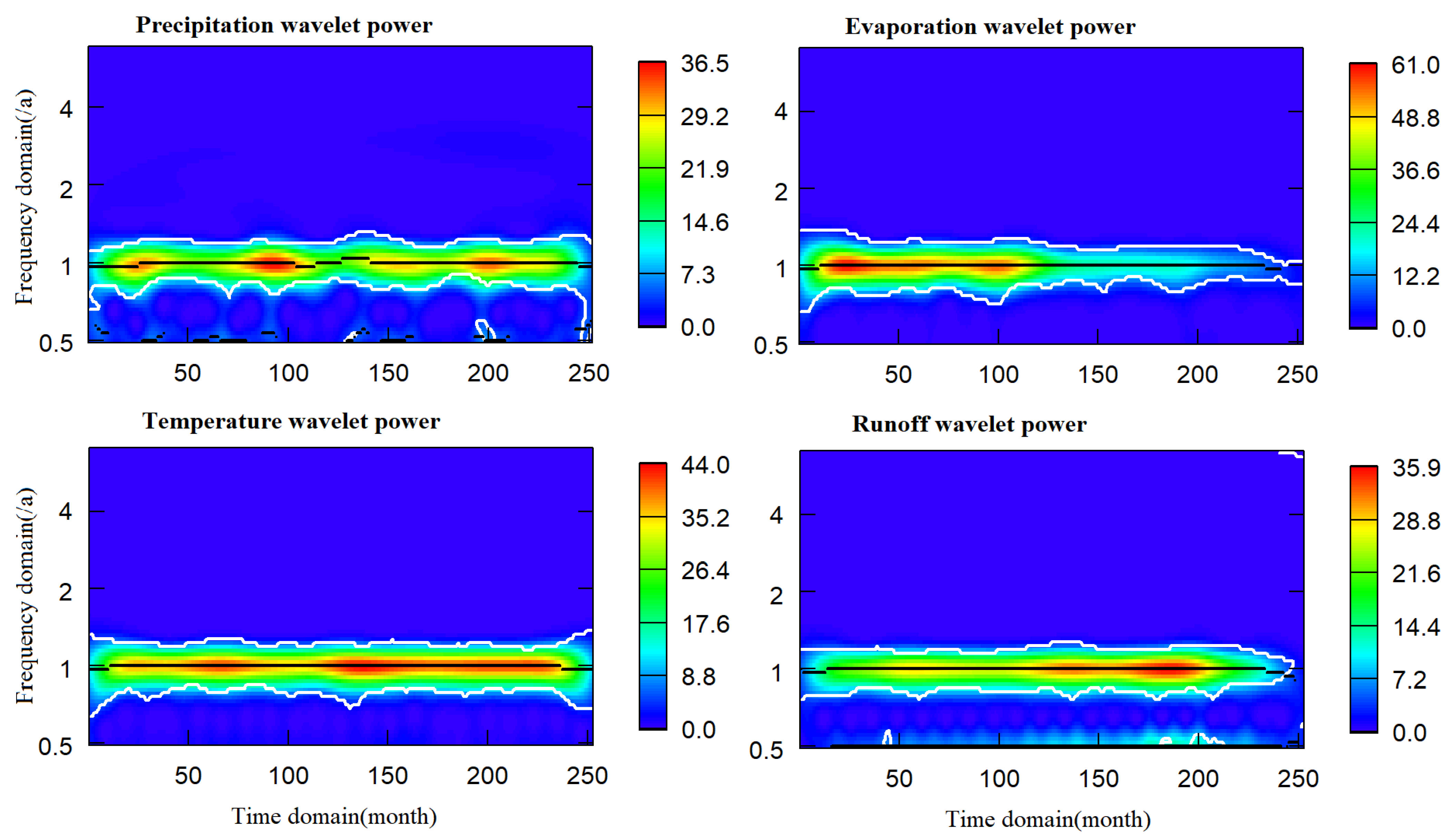
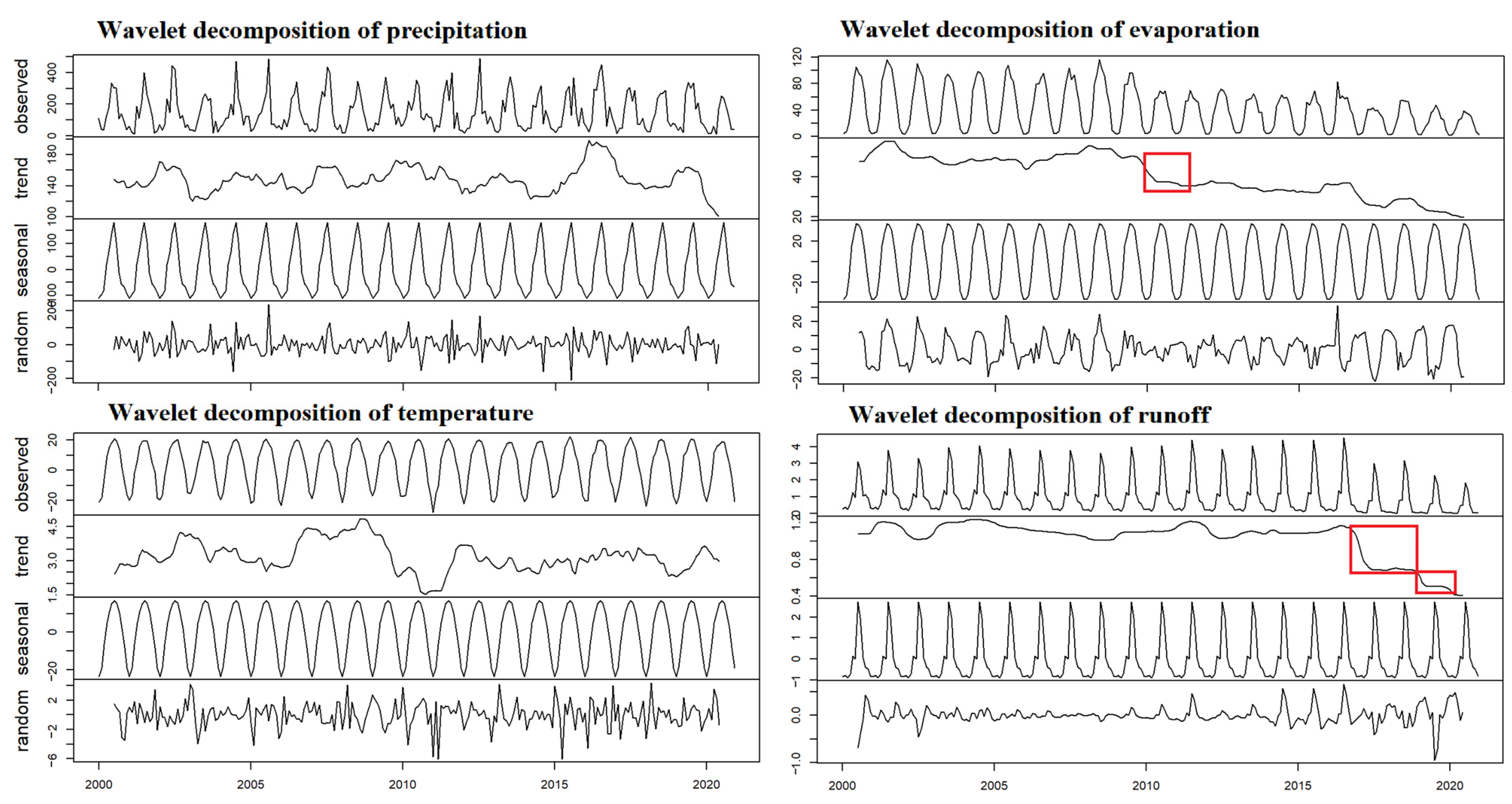
As is shown in Figure 2, wavelet analysis extracted the periodic characteristics of the selected meteorological elements, with 1a being the significant main period for each parameter (p < 0.05). The observed value of the parameters’ time series data is decomposed into a trend term, a seasonal term, and a random term. The trend item after wavelet decomposition shows that in the Manas River Basin, although the precipitation showed a continuous downward trend from 2016 to 2018, there is potential for recovery. The trend item coefficient of precipitation during the observation period remains between 0.8 and 1.1. Furthermore, the decrease in evaporation is a long-term trend, emerging slowly before 2016 and then becoming significant after 2016. Meanwhile, runoff showed a sudden change in 2016, with the trend term coefficient rapidly declining from 1.0 to 0.6. Conversely, the temperature value remained stable in time and space, as did the trend term coefficient of temperature, hovering between 0.95 and 1.05. For these parameters, the reliability of the downward trend of evaporation from 2010 to 2011 and the downward trend of runoff from 2016 to 2020 exceeds 0.99 (as marked in the red boxes in Figure 3).
The periodic decomposition (Figure 3) shows that the precipitation in the study region has good periodicity and strong seasonal characteristics, with more precipitation in summer and less in winter. Given the excellent stationarity of the area’s precipitation, EnKF has high reliability (>0.9) to predict its future trend. It is worth noting that the MK test and ACF show that the temperature is stable. During the entire observation period, the temperature at the 9 meteorological stations did not manifest a significant trend. However, the temperature data at the micro-scale shows strong periodic change characteristics. Therefore, the EnKF can reliably estimate the daily temperature data in the future and can predict the temperature in the next 25 days with a 98% confidence level. The performance of this method is 2 to 2.3 times that of the traditional weather forecast under the general circulation model.

4.3. Prediction

As described in Section 3.1, the monitoring data is iteratively calculated to provide a prediction with a probability distribution for the future data of each monitoring station in the Manas River Basin. Combined with spatial interpolation, short-term hydrometeorological parameter prediction can be provided for spatial points of interest. The model shows good performance in data aggregation.
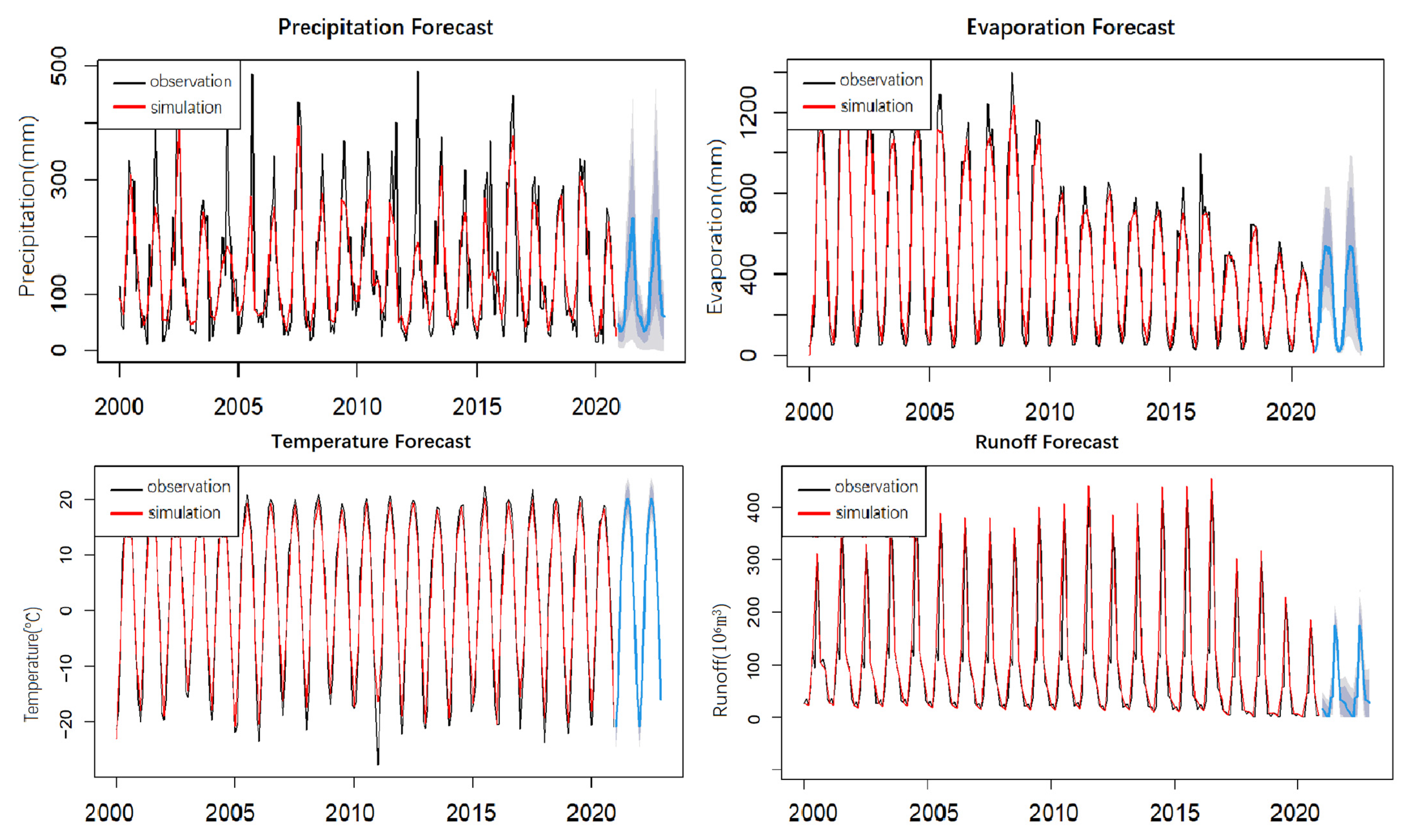
The values in Figure 4 are representative parameters used to describe the overall state of the basin obtained by applying the inverse distance weighted (IDW) average of the station data. By combining these data with the DEM data, the predicted values of the hydrometeorological parameters at specific locations can be restored. The forecast period, in this case, is 2 years, and the prediction values from 2000 to 2001 are extrapolated from the reverse time series. The NSE of the prediction model based on the EnKF for precipitation, evaporation, temperature, and runoff are 0.86, 0.89, 0.96, and 0.9, respectively. In comparison, the Nash efficiency coefficient of the original EnKF is 0.72, 0.85, 0.80, and 0.79.
In order to evaluate the prediction ability of the model, the cross-validation method proposed by Stone et al. is used [37]. The prediction is made for two years by applying the observation data from several years, and the prediction data is then compared with the real data. The data from 2011 to 2020 was divided into five periods. Next, the observation data of all meteorological elements before the data start time for each period (e.g., modeled the data from four meteorological elements before 2019 to provide predictions for the four meteorological elements from 2019 to 2020). The comparison between the prediction value and the real value is carried out after the model simulation.
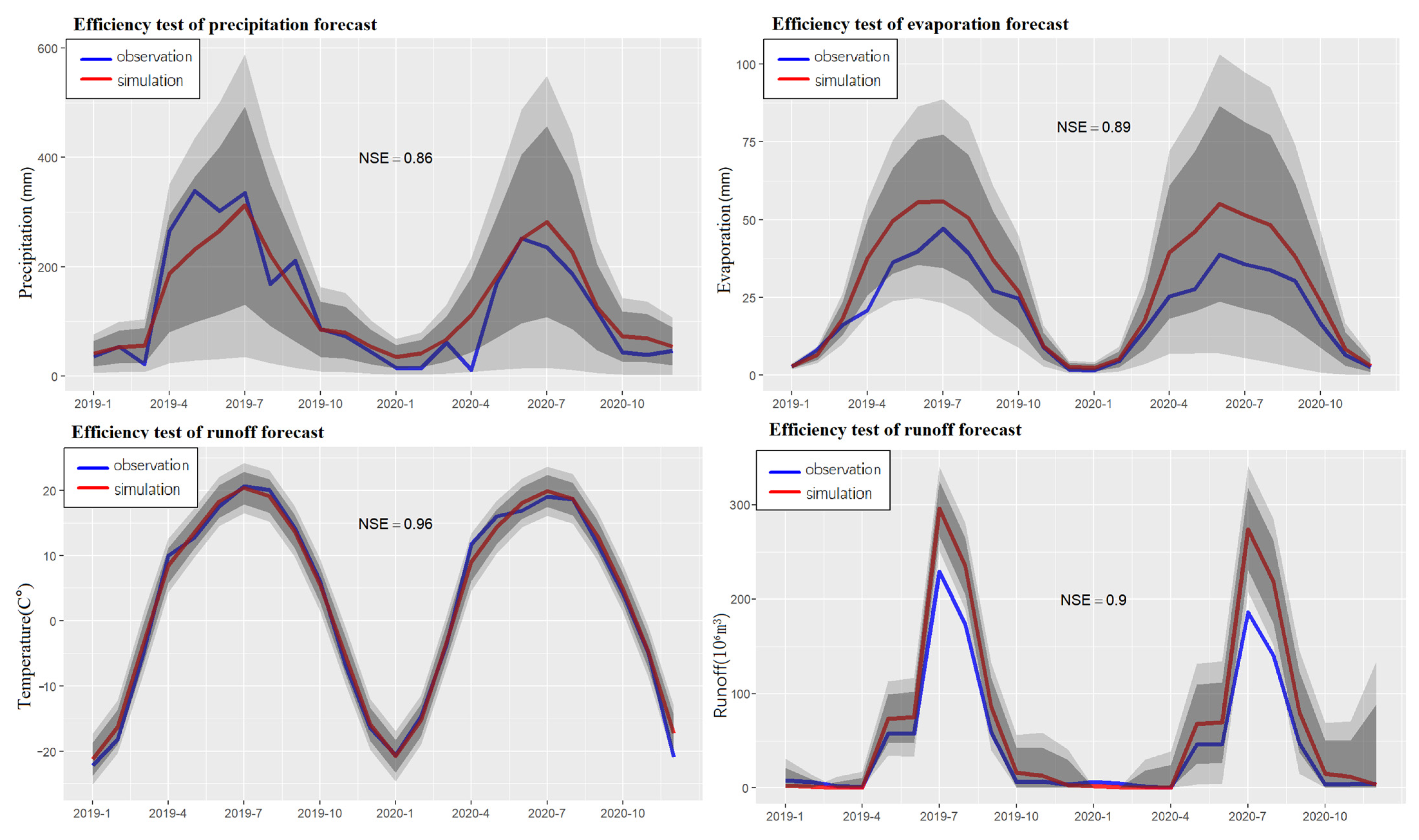
Figure 5 shows the test results of the last period (2019–2020). The dark gray area represents the 80% confidence interval of the predicted value and the light gray area represents the 95% confidence interval of the predicted value. When the EnKF forecasts each meteorological element, there is a major difference in uncertainty (see Figure 5). For example, the prediction of temperature and runoff is more confident, but the prediction of precipitation and evaporation is unreliable. Moradkhani et al. claim that the uncertainty of the filter in predicting different parameters is mainly related to the data resolution and correlation by using different parameter configurations in four catchments [38]. Generally speaking, the lower the uncertainty, the more accurate the prediction results will be. However, the specific relationship is greatly affected by the internal structure of the model [39], which relates to the balance means of variance error in Bayesian statistics. Finding a way to reduce the uncertainty will be valuable especially when high-precision multidimensional data is unavailable [40,41].

4.4. Reducing Data Overreliance and Improving Prediction Ability

Based on the results of the model application and error analysis, we conducted some investigations, which are helpful for further research. Reducing data overreliance and improving prediction ability are the most important tasks, considering their importance in forecasting hydrometeorological parameters and the limitations of the EnKF framework itself.
Data overreliance is a common problem in hydrological models, especially models driven by differential equations [6]. The requirements for data are mainly embodied in data integrity and data resolution. While using data assimilating, we can usually obtain the data we need by estimating the ensemble parameters and using the error covariance matrix to control the prediction uncertainty. However, data scientists have long been committed to mining more information from less data or inferring the ensemble properties from fewer samples. In general, the algorithm based on the optimal estimation of EnKF converges with an exponential rate while the covariance matrix used to control the error converges with a quadratic rate [19]. By using different forms of system equations and measurement equations, many variants of the Kalman filter were proposed to improve data utilization efficiency. For example, the single evolutionary interpolated Kalman filter (SEIK) proposed by Pham et al. [23], the error subspace statistical estimation (ESSE) proposed by Lermusiaux et al. [42], and the elastic transform Kalman filter (ETKF) proposed by Bishop et al. [43]. These modified models are applicable to different situations. Selecting the appropriate model through cross-validation may help to reduce data dependency.
Many studies have been devoted to improving the accuracy of the hydrometeorological prediction model. The results indicate that the prediction ability of the model on precipitation and evaporation could be promoted. An intuitive approach is to use a particle filter when high-resolution data are available [18]. In recent years, the deep learning method has achieved good results in prediction accuracy. Ghiasi et al. developed an artificial intelligence-based predictive model, coupling granular computing and neural network models (GrC-ANN) to provide a robust estimation of water head and its uncertainty for a range of flow geometric conditions with high spatiotemporal variability [44]. PINN (physics-informed neural network) considers both observation data and physical equations while giving an estimate with moderate efficiency. Application of the physics-informed DNNs to large-scale problems will require access to multi-GPU computers and scalable training algorithms, but the benefits in accuracy are considerable indeed [45].

4.5. Relationship between Precipitation and Altitude

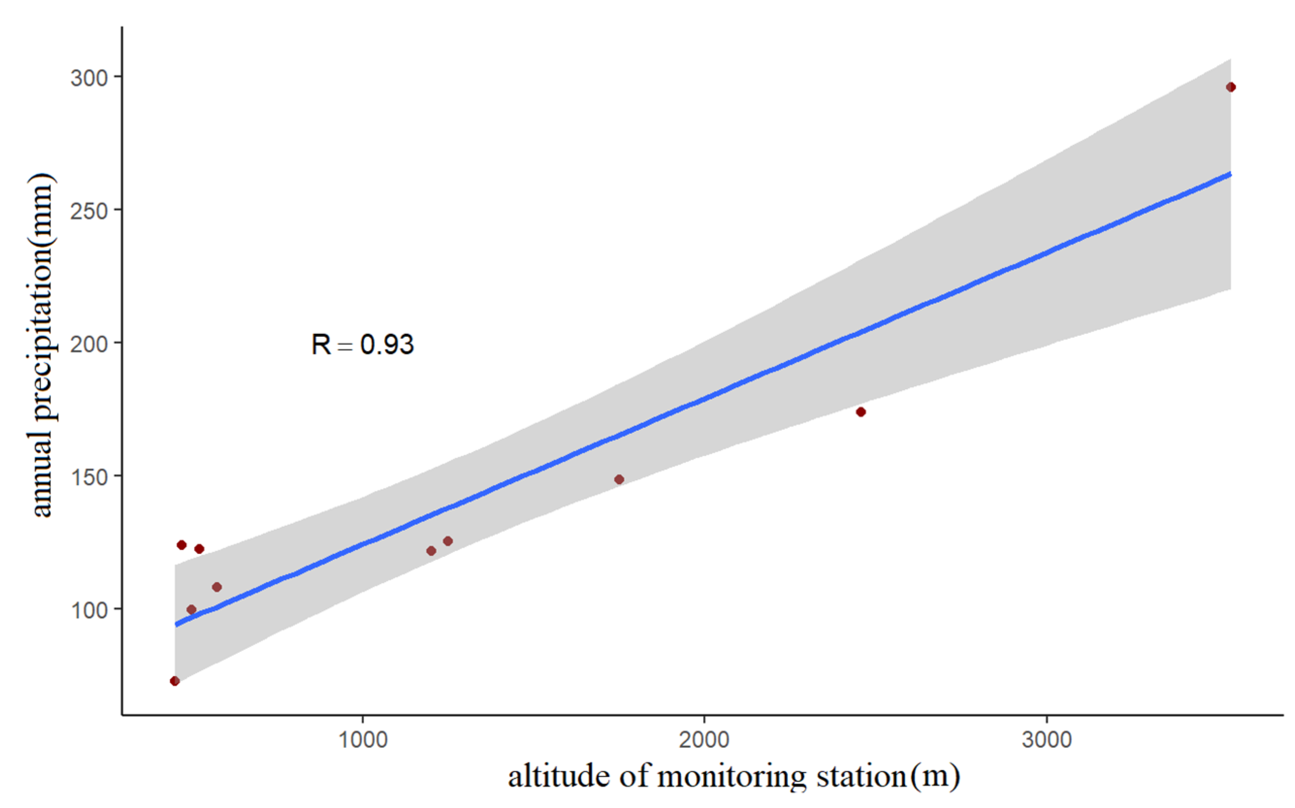
The study area is composed of the northern central plains area and the southern mountainous region, so the vertical zonal effect is significant. From the foot of the mountains, as the altitude increases, precipitation also gradually increases. After reaching the height of 3000 m, the water vapor in the air decreases due to a large amount of precipitation (Figure 6). Evaporation capacity then becomes weak due to the rapid reduction of temperature, resulting in high water vapor in the southern mountainous area of the study area all year round [15,36]. Monitoring station data shows that at an altitude of 2500 m or lower, annual average precipitation increases by 5.46 mm for every 100 m increase in altitude. Moreover, at an altitude exceeding 2500 m, the annual average precipitation increases by 7.82 mm for every 100 m increase in altitude.

4.6. Relationship between Evaporation and Temperature

Evaporation is mainly composed of water surface evaporation and soil-vegetation evaporation. The Dalton formula expresses that the evaporation rate of the evaporation dish is directly proportional to the wind speed and the saturated water vapor pressure difference and that the saturated water vapor pressure rises rapidly with the rise of temperature, and vice versa. The variation of saturated vapor pressure with temperature is larger at higher temperatures than at lower ones. Luo et al. show that when the temperature decreases from 30 °C to 25 °C, the saturated water vapor pressure decreases by 10.76 hPa, whereas when the temperature decreases from 15 °C to 10 °C, the saturated water vapor pressure only decreases by 4.77 hPa [46]. This scale effect (especially in areas with perennial rainless months) enables temperature variability to be transmitted to evaporation [4]. In the study area, the correlation coefficient between the two is 0.85. Although the relationship between evaporation and temperature is average, for the EnKF, the spatio-temporal dependence of such parameters can effectively improve the prediction performance of the model [47].

5. Conclusions

Climate change prediction has been the motivation for conducting studies on the possible impact of future climate change on the ecosystem (Yao et al. 2011). The various models currently in use show significant differences in regional prediction ability, and no climate model can simulate all meteorological elements with accuracy (Walsh et al. 2008). However, compared with single mode, multi-mode sets exhibit higher simulation ability and lower probability of error. Similar results were reported by Alemu et al. [2], Houtekamer et al. [47], Rodriguez et al. [48], and Wang et al. [49]. Ensemble data assimilation is an effective way to evaluate the uncertainty of model structure according to several studies [3,24,31,39]. The present study used hourly data of precipitation, evaporation, runoff, and temperature at nine stations in the Manas River Basin to investigate change trends and characteristics of hydrometeorological parameters in the region from 2000 to 2020. The EnKF is combined with a wavelet decomposition algorithm to calculate the optimal estimation of parameters and quantitative the prediction uncertainty. The research smoothly utilizes wavelet analysis as a preprocessing of the Ensemble Kalman Filter. The model’s NSE of precipitation, evaporation, temperature, and runoff reached 0.86, 0.89, 0.96, and 0.9 respectively. The BCIP index has not changed significantly compared with the original EnKF. At the same time, the K-S value has increased from 0.28 to 0.40.
During the observation period from 2000 to 2020, the precipitation, evaporation, and runoff of the Manas River Basin were stable for most of the first 10 years. However, the hydrological cycle was disturbed from 2009 to 2010, with precipitation showing a continuing downward trend. Evaporation dropped precipitously over the same time period. From 2010 to 2017, the stability of the runoff decreased, and evaporation further decreased. Runoff began to show a significant and continuous downward trend in 2017. Runoff was concentrated during the summer flood season, with changes in this time distribution expected to increase future flood intensity during the flood season. The probability of extreme climatic and hydrological events in the Manas River Basin, especially those related to runoff, has increased. In the last two years of the study period, compared with 2016, the probability of extremely low runoff increased by 37.62%.

Author Contributions

Conceptualization, G.H.; investigation, Y.C. and G.F.; Writing—original draft preparation, G.H.; writing—review and editing, Y.C., G.F. and Z.L. All authors have read and agreed to the published version of the manuscript.

Funding

The research was supported by the National Natural Science Foundation of China (Grant No. 42130512, No. 42071046).

Data Availability Statement

Hydrological data were obtained from National Climatic Data Center (NCDC): ftp://ftp.ncdc.noaa.gov/pub/data/noaa/isd-lite/ (accessed on 1 May 2022). The meteorological data and DEM data are from the China Meteorological Science Data Sharing Service Network: http://cdc.cma.gov.cn/ (accessed on 1 May 2022). Site information and other data were presented in the main text.

Acknowledgments

The authors gratefully acknowledge the Youth Innovation Promotion Association of the Chinese Academy of Sciences (2019431).

Conflicts of Interest

The authors declare no conflict of interest.

Appendix A

To solve the problem of estimation and decomposition of hydrometeorological parameters, wavelet decomposition is used to process the original data. The parameters are regarded as a stochastic vector sequence { X ( N , k ) } , and the target decomposition level is N, which conforms to the model:
x ( N , k + 1 ) = A ( N , k ) x ( N , k ) + ε ( N , k )
The observation process is:
v ( N , k ) = C ( N , k ) x ( N , k ) + η ( N , k )
where { ε ( N , k ) } and { η ( N , k ) } are independent zero mean Gaussian noise sequences, and the variances are { S ( N , k ) } and { T ( N , k ) } , respectively.
Given the observation { v ( N , k ) } , the method for estimating hydrometeorological parameters is: to find an estimate at the highest resolution level and then decompose it to different resolutions using wavelet transform. Here we only discuss the process of two-layer decomposition. Given the resolution of observation data, the decomposition from N-layer to N−1 and N−2 layer can be applied to other layers.
At time k, the stochastic vector sequence can be expanded as:
X _ k N = [ x ( N , k 3 ) , x ( N , k 2 ) , x ( N , k 1 ) , x ( N , k ) ] T
Assuming that the system equation and measurement Equations (A1) and (A2) are time-preserving on the decomposition layer, Their equivalent dynamic system can also be transformed as:
x ( N , k + 1 ) = A x ( N , k ) + ε ( N , k )
a set of expansions were attained through the same time structure:
x ( N , k + 1 ) = A 2 x ( N , k 1 ) + A ε ( N , k 1 ) + ε ( N , k )
x ( N , k + 1 ) = A 3 x ( N , k 2 ) + A 2 ε ( N , k 2 ) + A ε ( N , k 1 ) + ε ( N , k )
x ( N , k + 1 ) = A 4 x ( N , k 3 ) + A 3 ε ( N , k 3 ) + A 2 ε ( N , k 2 ) + A ε ( N , k 1 ) + ε ( N , k )
The average of Equations (A5)–(A7) indicates:
x ( N , k + 1 ) = 1 4 A 4 x ( N , k 3 ) + 1 4 A 3 x ( N , k 2 ) + 1 4 A 2 x ( N , k 1 ) + 1 4 A x ( N , k ) + ε ( 1 )
ε ( 1 ) = 1 4 A 3 ε ( N , k 3 ) + 1 2 A 2 ε ( N , k 2 ) + 3 4 A ε ( N , k 1 ) + ε ( N , k )
Implement (A8) and (A9) for different parameters, the result can be expressed in matrix form, which can be proved by calculation:
[ x ( N , k + 1 ) x ( N , k + 2 ) x ( N , k + 3 ) x ( N , k + 4 ) ] = [ 1 4 A 4 1 4 A 3 1 4 A 2 1 4 A 0 1 3 A 4 1 3 A 3 1 3 A 2 0 0 1 2 A 4 1 2 A 3 0 0 0 A 4 ] × [ x ( N , k 3 ) x ( N , k 2 ) x ( N , k 1 ) x ( N , k ) ] + [ ε ( 1 ) ε ( 2 ) ε ( 3 ) ε ( 4 ) ]
Equation (A10) can be abbreviated as:
x _ k + 1 N = A ¯ × x _ k N + W _ ¯ k N
ε(i), i = 2,3,4 are estimated remainder of hydrometeorological parameters. They have the same expression as Equation (A9).
For Equation (A11), the expectation and variance of the remainder satisfy:
E { W _ ¯ k N } = 0 ,   E { W _ ¯ k N ( W _ ¯ k N ) T } = Q ¯
where Q ¯ is a 4×4 symmetric matrix, and its elements could be calculated by a pyramidal algorithm [30]:
q 11 ¯ = 1 16 A 6 Q + 1 4 A 4 Q + 9 16 A 2 Q , q 12 ¯ = 1 6 A 5 Q + 1 2 A 3 Q + A Q , q 13 ¯ = 3 8 A 4 Q + A 2 Q , q 14 ¯ = A 3 Q , q 22 ¯ = 1 9 A 6 Q + 4 9 A 4 Q + A 2 Q + Q , q 23 ¯ = 1 3 A 5 Q + A 3 Q + A Q q 24 ¯ = A 4 Q + A 2 Q , q 33 ¯ = 1 4 A 6 Q + A 4 Q + A 2 Q + Q , q 34 ¯ = A 5 Q + A 3 Q + A Q q 44 ¯ = A 6 Q + A 4 Q + A 2 Q + Q
The measurement equation ruled by Equation (A11) is:
[ v ( N , k 3 ) v ( N , k 2 ) v ( N , k 1 ) v ( N , k ) ] = [ C 0 0 0 0 C 0 0 0 0 C 0 0 0 0 C ] × [ x ( N , k 3 ) x ( N , k 2 ) x ( N , k 1 ) x ( N , k ) ] + [ η ( N , k 3 ) η ( N , k 2 ) η ( N , k 1 ) η ( N , k ) ]
Also can be abbreviated as:
V _ k N = C ¯ × X _ k N + Π _ k N
The expectation and variance of the remainder satisfy:
E { Π _ k N } = 0 , E { Π _ k N ( Π _ k N ) T } = R = d i a g { R , R , R , R }
Using two-layer decomposition, the left side of Equation (A11) can be expressed as:
[ X _ k L N 2 X _ k H N 2 X _ k H N 1 ] = [ H N 2 H N 1 G N 2 H N 1 G N 1 ] X _ k N = T N 2 | N X k N  
Combined with the right side of Equation (A11):
[ X _ k + 1 L N 2 X _ k + 1 H N 2 X _ k + 1 H N 1 ] = A [ X _ k L N 2 X _ k H N 2 X _ k H N 1 ] + W _ k N
where the variables satisfy:
W _ k N = T N 2 | N W _ ¯ k N , E { W _ k N } = 0 , E { W _ k N ( W _ k N ) T } = Q A = T N 2 | N A ¯ ( T N 2 | N ) T , Q = T N 2 | N Q ¯ ( T N 2 | N ) T
Equation (A18) is the main motivation of this article, which described a preprocessing of a decomposable dynamic system. The measurement equation could be attained through Equation (A17) by a simple calculation:
V _ k N = C ¯ ( T N 2 | N ) T [ X _ k L N 2 X _ k H N 2 X _ k H N 1 ] + Π _ k N
So far, each decomposition quantity of the system Equation (A18) and measurement Equation (A19) has been obtained. The system equation and measurement equation can be processed using the ensemble Kalman filter to obtain the optimal estimation of these decomposition quantities. At the same time, because the remainder has a given variance structure, confidence intervals of these estimates can be constructed.

Appendix B

Appendix B will discuss the convergence and robustness of EnKF with wavelet decomposition. The same notation as Appendix A was used to avoid ambiguity.
We assume system Equation (A1) and measurement Equation (A2) are observable and controllable. The definitions of these two constraints (observable and controllable) for the system can be seen in the study of Moradkhani, H. et al. [38]. To put it simply, observable means the observation result of the system is a sufficient statistic of the change of the system. While controllability means that the control equation is nonsingular.
The estimation of innovation begins with its expansion:
F = y H ( x ¯ f ) = A ( I K C )
and the ensemble covariance follows:
( P m P ) ( P m P ) T = F m n 1 ( P n + 1 P ) B m B m T ( P n + 1 P ) ( F m n 1 ) T
If the system is a stationary process, it is obvious that the eigenvalue of F should be between −1 and 1. Therefore, Fkconvergence to zero matrix while k . On the other hand, P is a positive definite symmetric matrix. The trace of the left side in Equation (A22) can be constrained by:
tr ( P m P ) ( P m P ) T tr ( F m n 1 ( F m n 1 ) T ) × tr ( B m B m T + R ) C r m
where r is a constant between 0 and 1, C is a constant independent with r. The difference between Kalman gain matrix Km and its limit (if exists) can be calculated as:
K m K = P m C T ( C P m C T + R ) 1 P C T ( C P C T + R ) 1 = ( P m P ) C T ( C P m C T + R ) 1 + P C T [ ( C P m C T + R ) 1 ( C P C T + R ) 1 ] = ( P m P ) C T ( C P m C T + R ) 1 + P C T ( C P m C T + R ) 1 [ ( C P C T + R ) ( C P m C T + R ) ] ( C P C T + R ) 1 = ( P m P ) C T ( C P m C T + R ) 1 + P C T ( C P m C T + R ) 1 C ( P P m ) C T ( C P C T + R ) 1
by Cauchy inequality, it shows:
( A + B ) ( A + B ) 2 ( A A T + B B T )
Combine Equation (A24) with Equation (A25), it shows:
tr ( ( K m K ) ( K m K ) T ) 2 tr ( P m P ) ( P m P ) T tr ( C T C ( tr ( C P 0 C T + R ) 1 ) 2 ) + 2 tr ( P P T ) tr ( C T C ) ( tr ( C P 0 C T + R ) 1 ) 2 tr ( C C T ) tr ( ( P P m ) ( P P m ) T ) tr ( C T C ) tr ( ( C P C T + R ) 1 ( C P C T + R ) 1 ) C 1 tr ( ( P m P ) ( P m P ) T ) C 2 r m
where C1 and C2 are constants independent with m. This proves that the input provided by wavelet decomposition will get the asymptotic optimal estimation under EnKF processing, even if the covariance matrix of the measurement matrix may not be convergent. The first inequality of Equation (A26) can be used to provide the confidence interval of hydrometeorological parameter prediction for each time node m.

Appendix C

In Appendix C, the impact of new data was discussed to verify model stability. If these effects can be limited by the scale of data and characteristics of the new data itself, the algorithm has good stability. The common method to verify the stability of the model is analyzing the transfer of disturbance in the measurement equation [33]. In this study, this process was realized through matrix and vector operations. It begins with a one-step increase in the observation vector:
X m = A X m 1 + K ( v m C A X m 1 ) X ˜ m = A X ˜ m 1 + K m ( v m C A X ˜ m 1 ) A X ˜ m 1 + K ( v m C A X ˜ m 1 ) + ( K m K ) ( v m C A X ˜ m 1 )
where X ˜ m is the estimate after adding new data. Equation (A27) is an expansion of Equation (3). The estimated difference and the covariance matrix of the difference were used to measure the impact of new data. The difference can be calculated as:
Δ m = X ˜ m X m = A ( X ˜ m X m ) K C A ( X ˜ m X m ) + ( K m K ) ( C A X m 1 C A X ˜ m 1 ) = ( I G C ) A Δ m 1 + ( K m K ) ( C A ( R m R ˜ m ) )
It is assumed that the variances of measurement errors are independent of each other (a universal prior hypothesis in hydrometeorological prediction). The square of the difference is:
| | Δ m | | n 2 = [ ( I K C ) A ] | | Δ m | | n 2 [ ( I K C ) A ] T + ( K m K ) R ( K m K ) T + ( I K C ) A A T C T ( K m K ) T + ( K m K ) C A A T ( I K C ) T = F | | Δ m 1 | | n 2 F T + ( K m K ) ( K m K ) T + F B m 1 ( K m K ) T + ( K m K ) B m 1 T F T
Perform iteration on Equation (A29), it showed:
| | Δ m | | n 2 = F m | | Δ 0 | | F m T + i = 0 m 1 F i ( K m i K ) ( K k i K ) T ( F i ) T + i = 0 m 1 F i [ F B m 1 i ( K m i K ) T + ( K m i K ) B m 1 i T F T ] ( F i ) T
At last, the trace of the difference can be limited by:
tr | | Δ m | | n 2 tr | | Δ m | | n 2 tr ( F k ( F k ) T ) + i = 0 m 1 tr ( F i ( F i ) T ) tr ( K m 1 K ) ( K m 1 K ) T + i = 0 m 1 tr ( F i ( F i ) T ) tr [ F B m 1 i ( K m i K ) T + ( K m i K ) B m 1 i T F T ] tr | | Δ 0 | | n 2 C 3 r 3 m + i = 0 m 1 C 4 r 4 i C 5 r 5 m i + i = 0 m 1 C 6 r 6 i C 7 r 7 m i + 1 C 8 r 8 8
where 0 < r3, r4, r5, r6, r7 < 1, r8 = max(r3, r4, r5, r6, r7), C3, …, C8 are constants independent of m, i and each other. It can be seen from Equation (A31) that the robustness of the model varies in different application scenarios. The instability brought by the new data was provided by multiple structures of both the system equation and measurement equation. However, at least in theory, the robustness of the model is excellent.

References

  1. Berghuijs, W.; RA, W.; Hrachowitz, M. A precipitation shift from snow towards rain leads to a decrease in streamflow. Nat. Clim. Change 2014, 4, 583–586. [Google Scholar] [CrossRef] [Green Version]
  2. Alemu, Z.; Dioha, M. Climate change and trend analysis of temperature: The case of Addis Ababa, Ethiopia. Environ. Syst. Res. 2020, 9, 27. [Google Scholar] [CrossRef]
  3. Stocker, T. Climate Change 2013: The Physical Science Basis: Working Group I Contribution to the Fifth Assessment Report of the Intergovernmental Panel on Climate Change; Cambridge University Press: Cambridge, UK, 2014; pp. 127–129. [Google Scholar]
  4. Chen, Y.; Li, Z.; Fan, Y.; Wang, H.; Deng, H. Progress and prospects of climate change impacts on hydrology in the arid region of northwest China. Environ. Res. 2015, 139, 11–19. [Google Scholar] [CrossRef] [PubMed]
  5. Kraft, B.; Jung, M.; Körner, M.; Koirala, S.; Reichstein, M. Towards hybrid modeling of the global hydrological cycle. Hydrol. Earth Syst. Sci. 2022, 36, 1576–1614. [Google Scholar] [CrossRef]
  6. Fang, G.; Yang, J.; Chen, Y.; Zammit, C. Comparing bias correction methods in downscaling meteorological variables for a hydrologic impact study in an arid area in China. Hydrol. Earth Syst. Sci. 2015, 19, 2547–2559. [Google Scholar] [CrossRef] [Green Version]
  7. Chen, Y.; Wang, H.; Wang, Z.; Zhang, H. Characteristics of extreme climatic/hydrological events in the arid region of northwestern China. Arid. Land Geogr. 2017, 40, 1–9. [Google Scholar]
  8. Chen, L.; Cao, Y.; Ma, L.; Zhang, J. A Deep Learning-Based Methodology for Precipitation Nowcasting with Radar. Earth Space Sci. 2020, 7, e2019EA000812. [Google Scholar] [CrossRef] [Green Version]
  9. Goodarzi, D.; Abolfathi, S.; Borzooei, S. Modelling solute transport in water disinfection systems: Effects of temperature gradient on the hydraulic and disinfection efficiency of serpentine chlorine contact tanks. J. Water Process Eng. 2020, 37, 101411. [Google Scholar] [CrossRef]
  10. Goodarzi, D.; Mohammadian, A.; Pearson, J.; Abolfathi, S. Numerical modelling of hydraulic efficiency and pollution transport in waste stabilization ponds. Ecol. Eng. 2022, 182, 106702. [Google Scholar] [CrossRef]
  11. Cazelles, B.; Chavez, M.; Berteaux, D.; Ménard, F.; Vik, J.; Jenouvrier, S.; Stenseth, N. Wavelet analysis of ecological time series. Oecologia 2008, 156, 287–304. [Google Scholar] [CrossRef] [PubMed]
  12. Hewlett, J.D.; Hibbert, A.R. Factors affecting the response of small watersheds to precipitation in humid areas. For. Hydrol. 1967, 1, 275–290. [Google Scholar]
  13. Abbott, M.; Bathurst, J.; Cunge, J.; O’connell, P.; Rasmussen, J. An introduction to the European Hydrological System—Systeme Hydrologique Europeen,“SHE”, 2: Structure of a physically-based, distributed modelling system. J. Hydrol. 1986, 87, 61–77. [Google Scholar] [CrossRef]
  14. Laio, F.; Di Baldassarre, G.; Montanari, A. Model selection techniques for the frequency analysis of hydrological extremes. Water Resour. Res. 2009, 45, W07416. [Google Scholar] [CrossRef]
  15. Chen, H.; Chen, Y.; Li, W.; Li, Z. Quantifying the contributions of snow/glacier meltwater to river runoff in the Tianshan Mountains, Central Asia. Glob. Planet. Change 2019, 174, 47–57. [Google Scholar] [CrossRef]
  16. Xie, X.; Zhang, D. Data assimilation for distributed hydrological catchment modeling via ensemble Kalman filter. Adv. Water Resour. 2010, 33, 678–690. [Google Scholar] [CrossRef]
  17. Clark, M.; Rupp, D.; Woods, R.; Zheng, X.; Ibbitt, R.; Slater, A.; Schmidt, J.; Uddstrom, M.J. Hydrological data assimilation with the ensemble Kalman filter: Use of streamflow observations to update states in a distributed hydrological model. Adv. Water Resour. 2008, 31, 1309–1324. [Google Scholar] [CrossRef]
  18. Vetra-Carvalho, S.; Van Leeuwen, P.J.; Nerger, L.; Barth, A.; Altaf, M.U.; Brasseur, P.; Kirchgessner, P.; Beckers, J.M. State-of-the-art stochastic data assimilation methods for high-dimensional non-Gaussian problems. Tellus A Dyn. Meteorol. Oceanogr. 2018, 70, 1–43. [Google Scholar] [CrossRef] [Green Version]
  19. Bannister, R.N. A review of operational methods of variational and ensemble-variational data assimilation. Q. J. R. Meteorol. Soc. 2017, 143, 607–633. [Google Scholar] [CrossRef] [Green Version]
  20. Houtekamer, P.L.; Zhang, F. Review of the Ensemble Kalman Filter for Atmospheric Data Assimilation. Mon. Weather. Rev. 2016, 144, 208–239. [Google Scholar] [CrossRef]
  21. Evensen, G. Sequential data assimilation with a nonlinear quasi-geostrophic model using Monte Carlo methods to forecast error statistics. J. Geophys. Res. Ocean. 1994, 99, 10143–10162. [Google Scholar] [CrossRef]
  22. Burgers, G.; Leeuwen, P.J.; Evensen, G. Analysis scheme in the ensemble Kalman filter. Mon. Weather. Rev. 1998, 126, 1719–1724. [Google Scholar] [CrossRef]
  23. Pham, D.T.; Verron, J.; Gourdeau, L. A singular evolutive Kalman filters for data assimilation in oceanography. J. Mar. Syst. 1998, 16, 323–340. [Google Scholar] [CrossRef]
  24. Kong, L.; Tang, X.; Zhu, J.; Wang, Z.; Pan, Y.; Wu, H.; Wu, L.; Wu, Q.; He, Y.; Tian, S. Improved inversion of monthly ammonia emissions in China based on the Chinese ammonia monitoring network and ensemble Kalman filter. Environ. Sci. Technol. 2019, 53, 12529–12538. [Google Scholar] [CrossRef] [PubMed]
  25. Chatrabgoun, O.; Karimi, R.; Daneshkhah, A.; Abolfathi, S.; Nouri, H.; Esmaeilbeigi, M. Copula-based probabilistic assessment of intensity and duration of cold episodes: A case study of Malayer vineyard region. Agric. For. Meteorol. 2020, 295, 108150. [Google Scholar] [CrossRef]
  26. Donnelly, J.; Abolfathi, S.; Pearson, J.; Chatrabgoun, O.; Daneshkhah, A. Gaussian process emulation of spatio-temporal outputs of a 2D inland flood model. Water Res. 2022, 225, 119100. [Google Scholar] [CrossRef] [PubMed]
  27. Naumann, G.; Cammalleri, C.; Mentaschi, L.; Feyen, L. Increased economic drought impacts in Europe with anthropogenic warming. Nat. Clim. Change 2021, 11, 485–491. [Google Scholar] [CrossRef]
  28. Hamid, A.; Hafeez, A.; Khan, M.; Alshomrani, A.; Alghamdi, M. Heat transport features of magnetic water–graphene oxide nanofluid flow with thermal radiation: Stability Test. Eur. J. Mech.-B/Fluids 2019, 76, 434–441. [Google Scholar] [CrossRef]
  29. Vishwanath, M. The recursive pyramid algorithm for the discrete wavelet transform. IEEE Trans. Signal Process. 1994, 42, 673–676. [Google Scholar] [CrossRef]
  30. Kalman, R.E. On the General Theory of Control Systems. IFAC Proceedings Volumes. 1960, 1, 491–502. [Google Scholar] [CrossRef]
  31. Sun, Y.; Bao, W.; Valk, K.; Brauer, C.C.; Sumihar, J.; Weerts, A.H. Improving forecast skill of lowland hydrological models using ensemble Kalman filter and unscented Kalman filter. Water Resour. Res. 2020, 56, e027468. [Google Scholar] [CrossRef]
  32. Farahani, A.V.; Abolfathi, S. Sliding Mode Observer Design for decentralized multi-phase flow estimation. Heliyon 2022, 8, e08768. [Google Scholar] [CrossRef] [PubMed]
  33. Nash, J.E.; Sutcliffe, J.V. River flow forecasting through conceptual models part IA discussion of principles. J. Hydrol. 1970, 10, 282–290. [Google Scholar] [CrossRef]
  34. Sornette, D.; Davis, A.; Ide, K.; Vixie, K.; Pisarenko, V.; Kamm, J. Algorithm for model validation: Theory and applications. Proc. Natl. Acad. Sci. 2007, 104, 6562–6567. [Google Scholar] [CrossRef] [Green Version]
  35. Massey, F.J., Jr. The Kolmogorov-Smirnov test for goodness of fit. J. Am. Stat. Assoc. 1951, 46, 68–78. [Google Scholar] [CrossRef]
  36. Wu, K. Hydrological Characteristics of Manas River Basin in Xinjiang. Inn. Mong. Water Resour. 2011, 6, 2. Available online: http://qikan.cqvip.com/Qikan/Article/Detail?id=40642448 (accessed on 1 June 2022).
  37. Stone, M. Cross-validatory choice and assessment of statistical predictions. J. R. Stat. Soc. Ser. B (Methodol.) 1974, 36, 111–133. [Google Scholar] [CrossRef]
  38. Moradkhani, H.; Sorooshian, S.; Gupta, H.V.; Houser, P.R. Dual state–parameter estimation of hydrological models using ensemble Kalman filter. Adv. Water Resour. 2005, 28, 135–147. [Google Scholar] [CrossRef] [Green Version]
  39. Tiao, G.C.; Tsay, R.S. Model specification in multivariate time series. J. R. Stat. Soc. Ser. B (Methodol.) 1989, 51, 157–195. [Google Scholar] [CrossRef]
  40. Yao, F.; Qin, P.; Zhang, J. Uncertainties in agricultural impact assessment of climate change based on model simulation and treatment methods. Sci. Bull. 2011, 56, 9. [Google Scholar] [CrossRef] [Green Version]
  41. Walsh, J.E.; Chapman, W.L.; Romanovsky, V.; Christensen, J.H.; Stendel, M. Global climate model performance over Alaska and Greenland. J. Clim. 2008, 21, 6156–6174. [Google Scholar] [CrossRef]
  42. Lermusiaux, P.; Robinson, A. Data assimilation via error subspace statistical estimation. Part I: Theory and schemes. Mon. Weather. Rev. 1999, 127, 1385–1407. [Google Scholar] [CrossRef]
  43. Bishop, C.; Etherton, B.; Majumdar, S. Adaptive sampling with the ensemble transform Kalman filter. Part I: Theoretical aspects. Mon. Weather. Rev. 2001, 129, 420–436. [Google Scholar] [CrossRef]
  44. Ghiasi, B.; Noori, R.; Sheikhian, H.; Zeynolabedin, A.; Sun, Y.; Jun, C.; Hamouda, M.; Bateni, S.M.; Abolfathi, S. Uncertainty quantification of granular computing-neural network model for prediction of pollutant longitudinal dispersion coefficient in aquatic streams. Sci. Rep. 2022, 12, 4610. [Google Scholar] [CrossRef] [PubMed]
  45. Chen, Z.; Liu, Y.; Sun, H. Physics-informed learning of governing equations from scarce data. Nat. Commun. 2021, 12, 1–13. [Google Scholar] [CrossRef] [PubMed]
  46. Luo, L.; Wang, X.; Yu, P. Comparative study on calculation formulas of saturated water vapor pressure. Meteorol. Hydrol. Mar. Instrum. 2003, 4, 4. Available online: http://qikan.cqvip.com/Qikan/Article/Detail?id=8938748 (accessed on 1 June 2022).
  47. Houtekamer, P.L.; Mitchell, H.L. Data assimilation using an ensemble Kalman filter technique. Mon. Weather. Rev. 1998, 126, 796–811. [Google Scholar] [CrossRef]
  48. Rodriguez-Iturbe, I.; Mejía, J.M. On the transformation of point rainfall to areal rainfall. Water Resour. Res. 1974, 10, 729–735. [Google Scholar] [CrossRef]
  49. Wang, J.; Zhang, M.; Wang, S. Change of snowfall/rainfall ratio in the Tibetan Plateau based on a gridded dataset with high resolution during 1961–2013. Acta Geo-Graph. Sin. 2016, 71, 142–152. [Google Scholar]
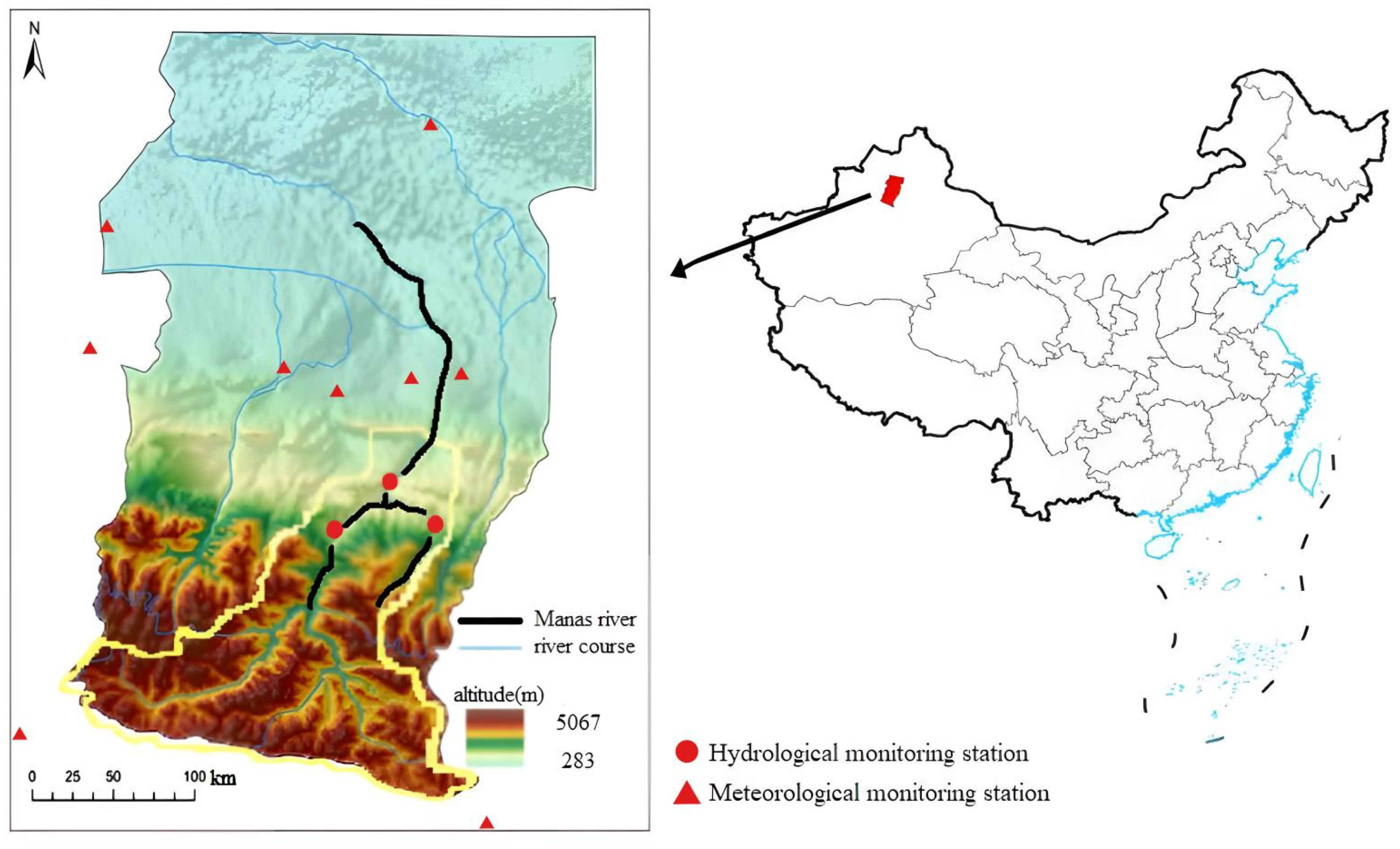
Figure 1. Sites in the study area, with DEM distribution. The map is from Chinese Standard Map (http://bzdt.ch.mnr.gov.cn/, GS (2019)1822 (accessed on 22 November 2022))
Water 14 03970 g001
Figure 2. Wavelet power diagram of meteorological parameters from 2000 to 2020.
Water 14 03970 g002
Figure 3. Periodic wavelet decomposition based on multi-year moving average. The red boxes represent significant downtrends, which were observed by stationarity test.
Water 14 03970 g003
Figure 4. Monthly data forecast for four hydrological parameters using EnKF.
Water 14 03970 g004
Figure 5. Predictions and confidence intervals at two levels (0.8 and 0.95) with EnKF.
Water 14 03970 g005
Figure 6. Relationship between precipitation and altitude. In the figure, the blue line is the regression line which represents the optimal parameters, the gray area is enclosed by the upper and lower confidence bounds under the 0.95 confidence level, and the red points represent the meteorological station.
Water 14 03970 g006
Table 1. Longitude, latitude, and altitude data of 9 monitoring stations in the study area.
Site NameLongitudeLatitudeAltitude (m)
Karamay84°51′45°37′449.5
Shawan85°37′44°20′522.2
Manas86°12′44°19′471.4
Hutubi86°51′44°10′575.1
Daxigou86°50′43°06′3539.0
Bayanbulak84°09′43°02′2458.0
Baluntai86°18′44°19′1739.0
Ulan Wusu84°62′44°45′480.6
Shihezi86°02′44°18′493.0
Table 2. Stationarity test of four hydrological parameters from 2010 to 2020 (p < 0.05).
ParameterTest20102011201220132014201520162017201820192020
PrecipitationMK0.0880.0640.209−0.0370.099−0.035−0.060.49−0.047−0.089−0.08
ACF0.0320.0640.238−0.0630.0890.024−0.384−0.28−0.097−0.03−0.606
EvaporationMK−0.317−0.0920.098−0.0850.0440.0350.021−0.1320.0330.07−0.017
ACF−0.755−0.746−0.026−0.0630.0240.026−0.422−0.177−0.2370.045−0.211
TemperatureMK0.07−0.0990.037−0.037−0.0940.0820.064−0.363−0.039−0.033−0.251
ACF−0.048−0.068−0.0740.0020.0990.0540.034−0.46−0.195−0.27−0.256
RunoffMK0.002−0.0080.01−0.001−0.0010.001−0.0060.0020.0040.0060.002
ACF0.004−0.007−0.00900.001000.0090.01−0.0040.008
Publisher’s Note: MDPI stays neutral with regard to jurisdictional claims in published maps and institutional affiliations.