
Correlation between Ground Measurements and UAV Sensed Vegetation Indices for Yield Prediction of Common Bean Grown under Different Irrigation Treatments and Sowing Periods
 ,
,  , and
, and 
Abstract
:1. Introduction
2. Materials and Methods
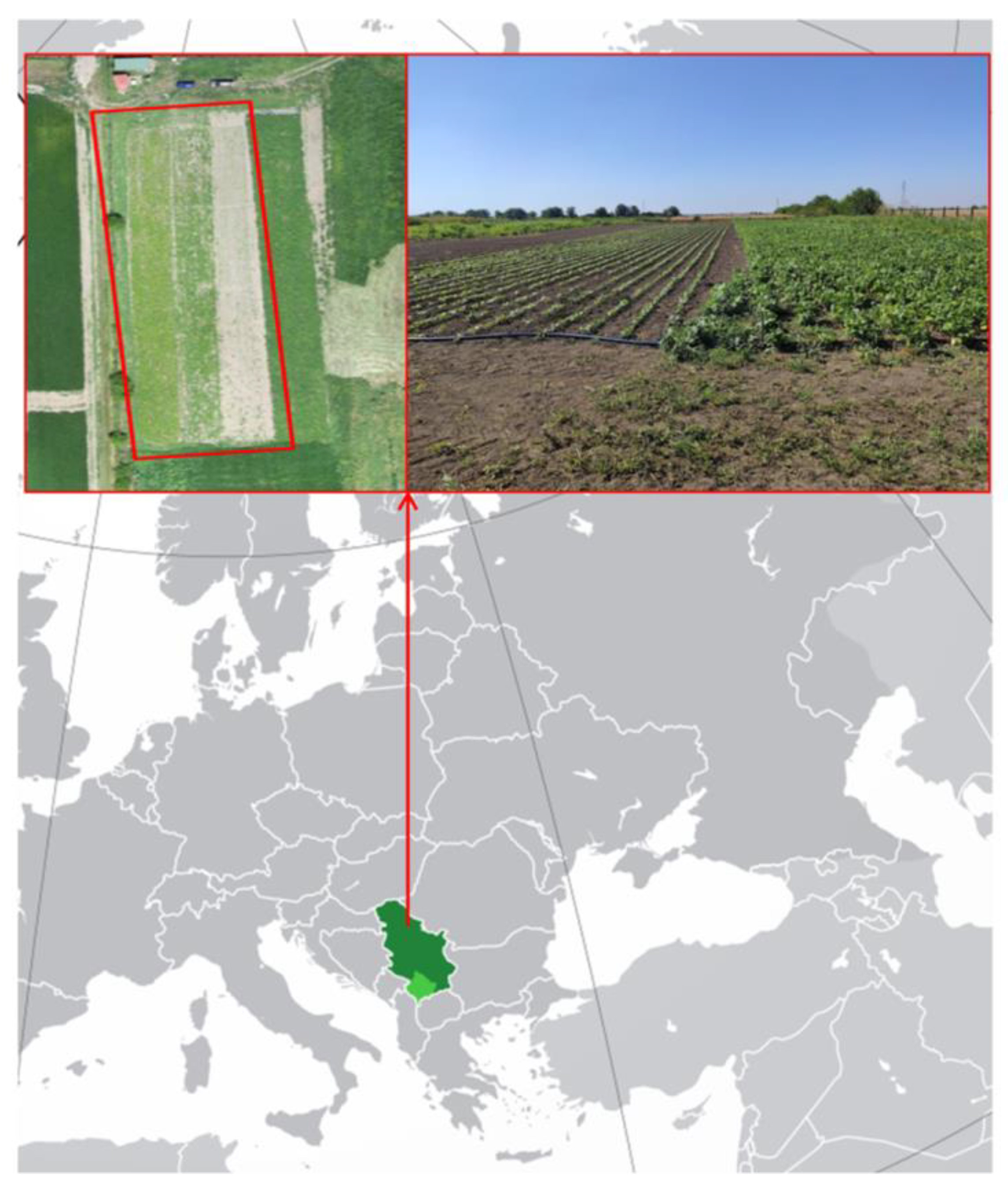
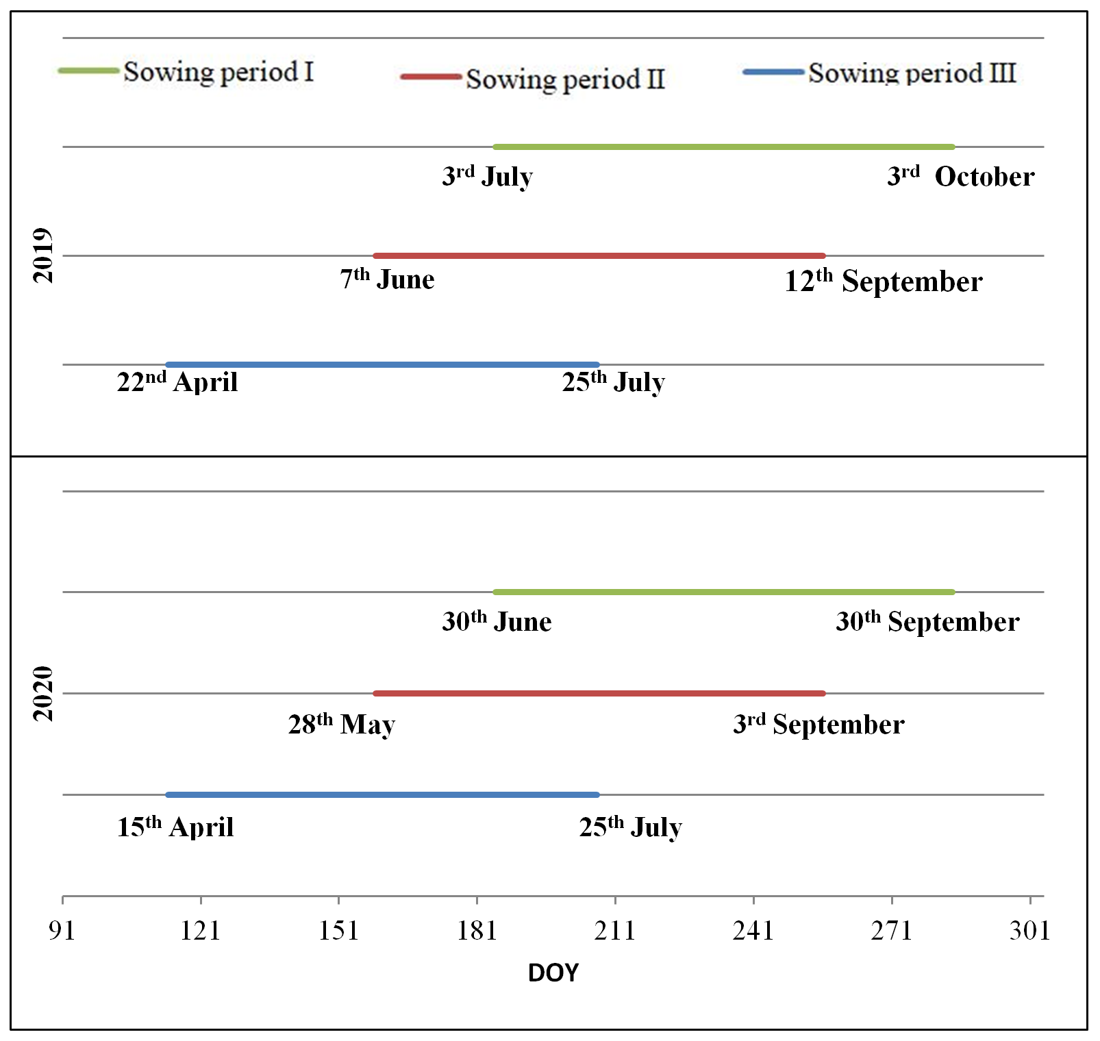
2.1. Study Area
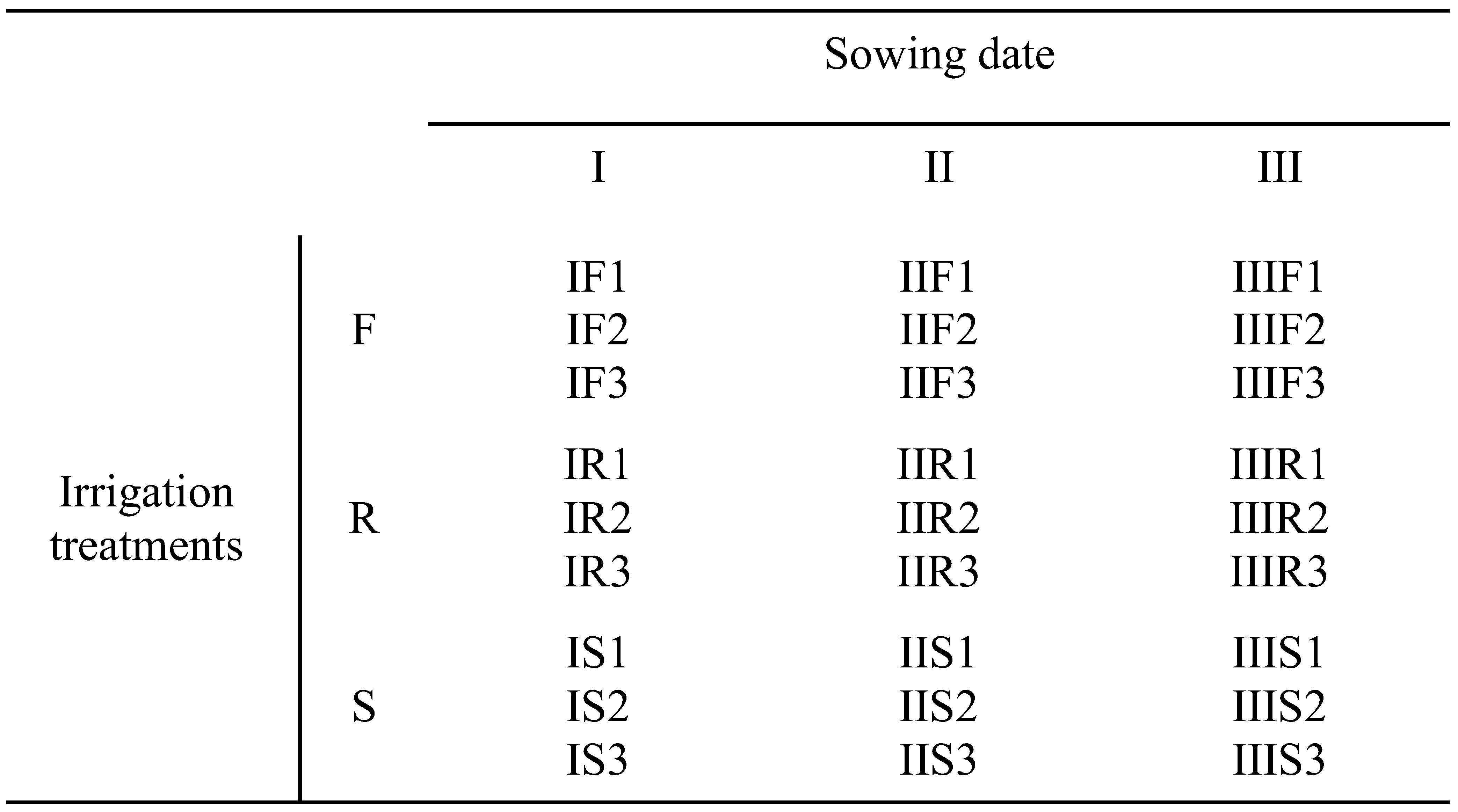
2.2. Experiment Design
2.3. Ground Monitoring
2.3.1. Meteorological Observations
2.3.2. Evapotranspiration
2.3.3. Soil Moisture
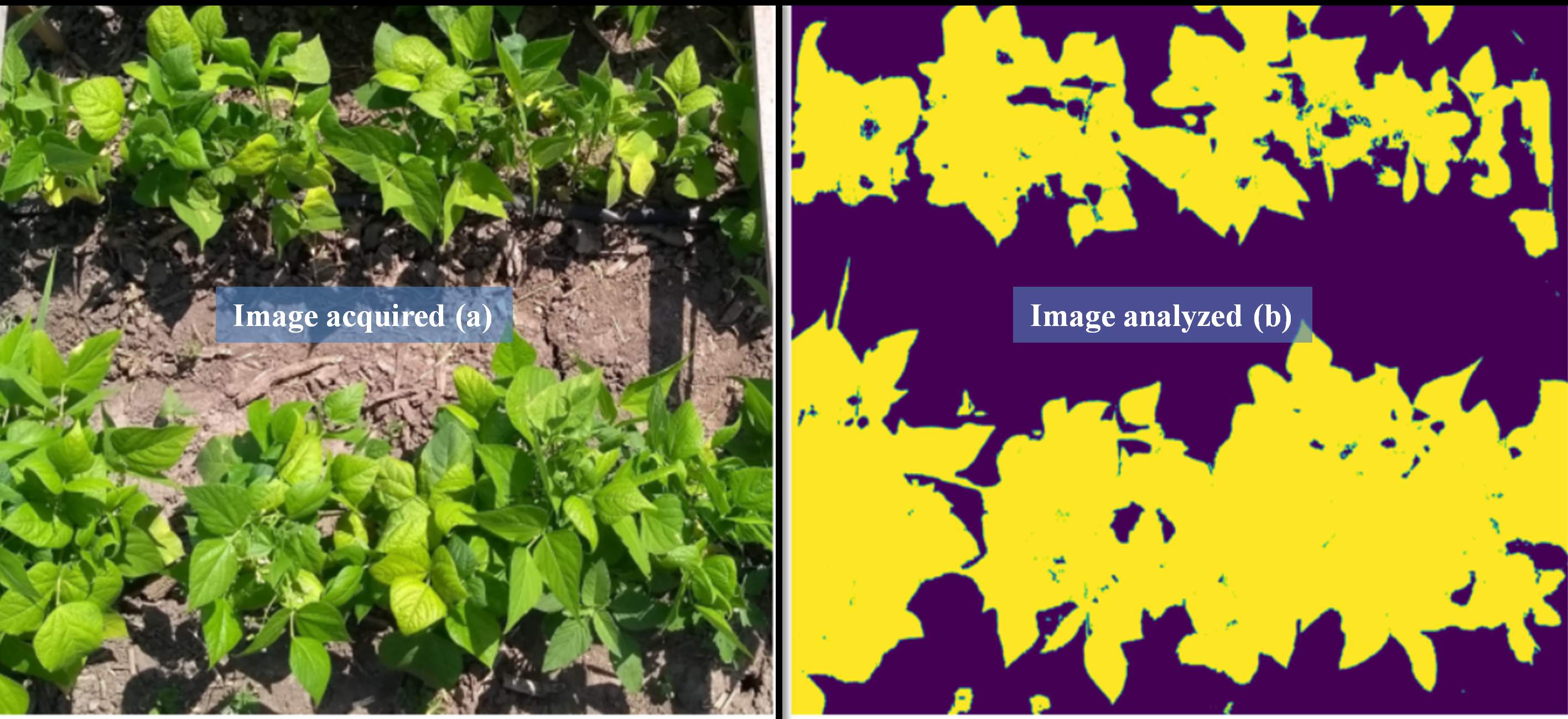
2.3.4. Canopy Cover (CC)
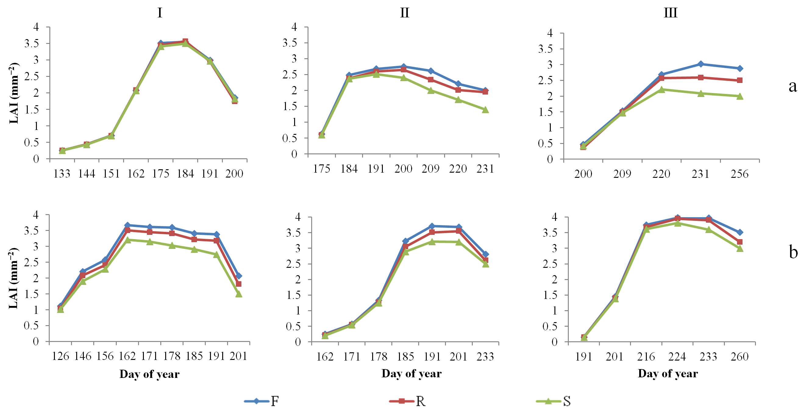
2.3.5. Leaf Area Index (LAI)
2.4. Vegetation Indices (VI) Determined from UAV Multispectral Imagery
2.4.1. UAV Image Acquisition
2.4.2. Image Processing and Computation of Vegetation Indices
2.5. Data Processing
3. Results
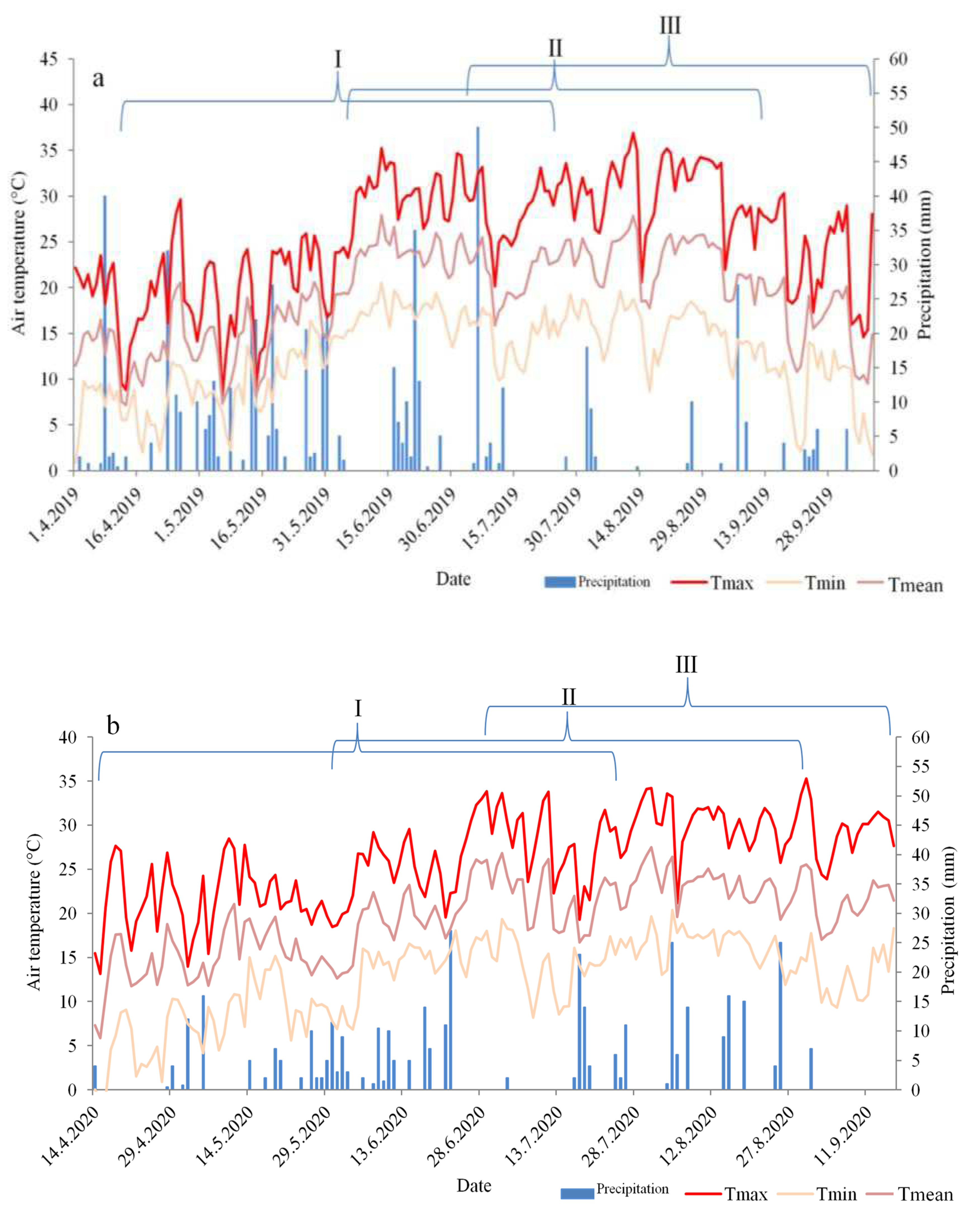
3.1. Climate
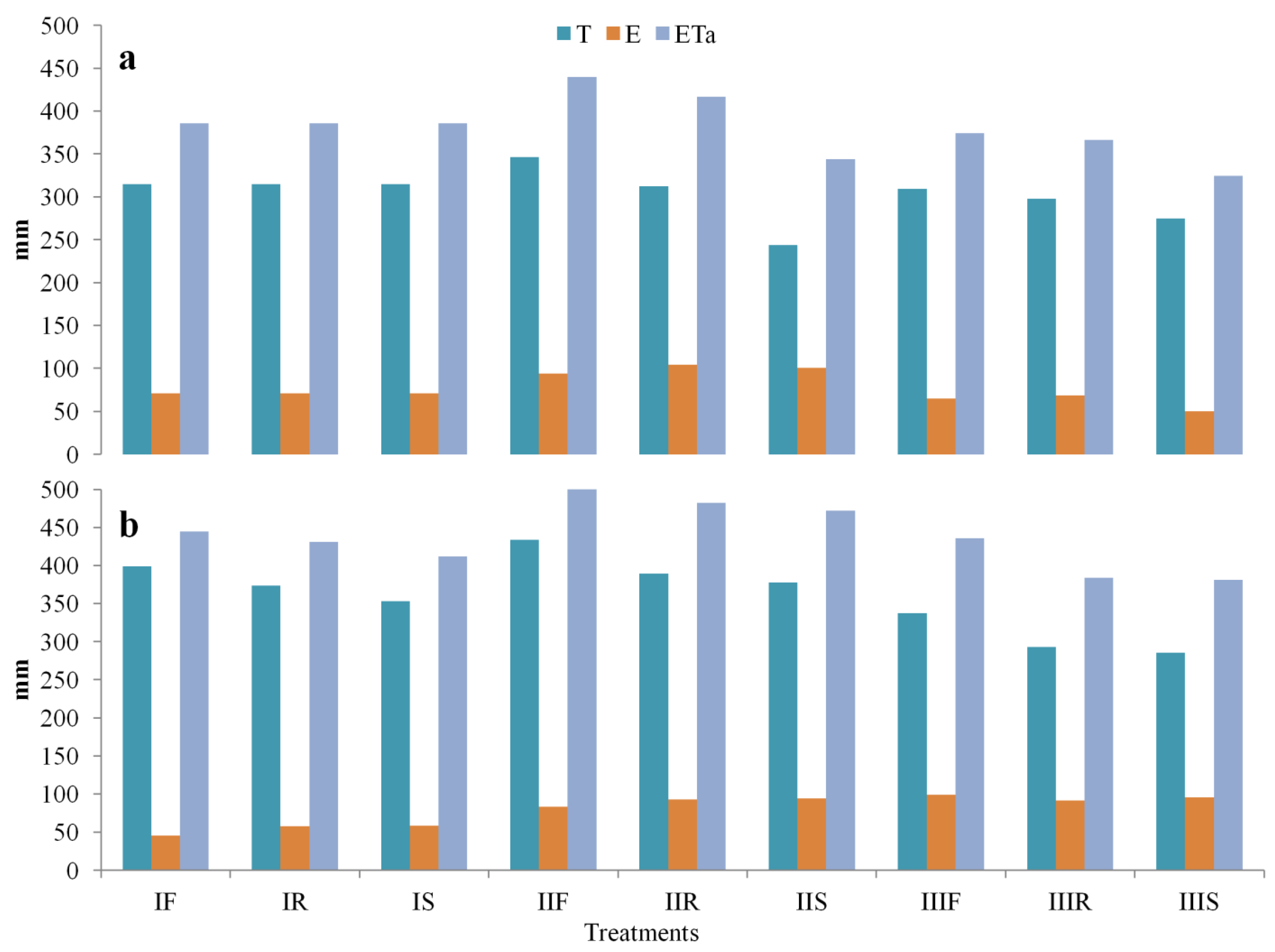
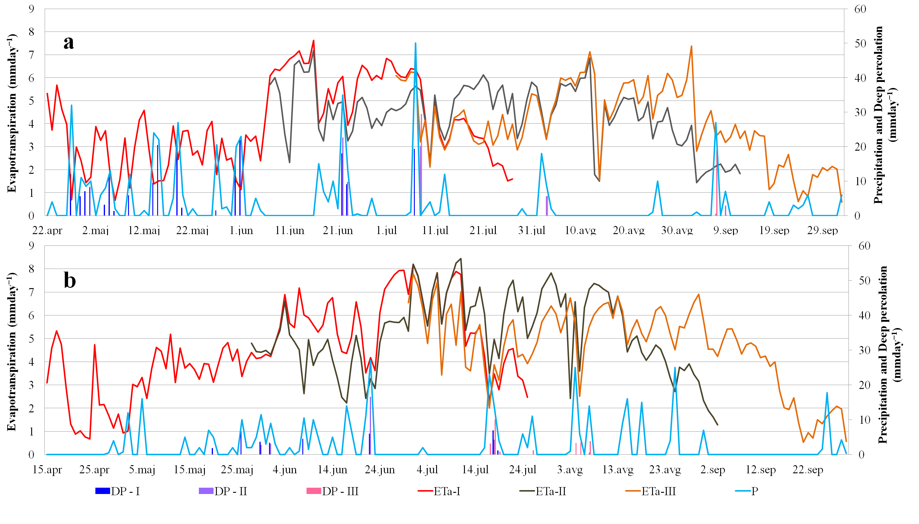
3.2. Transpiration and Evaporation
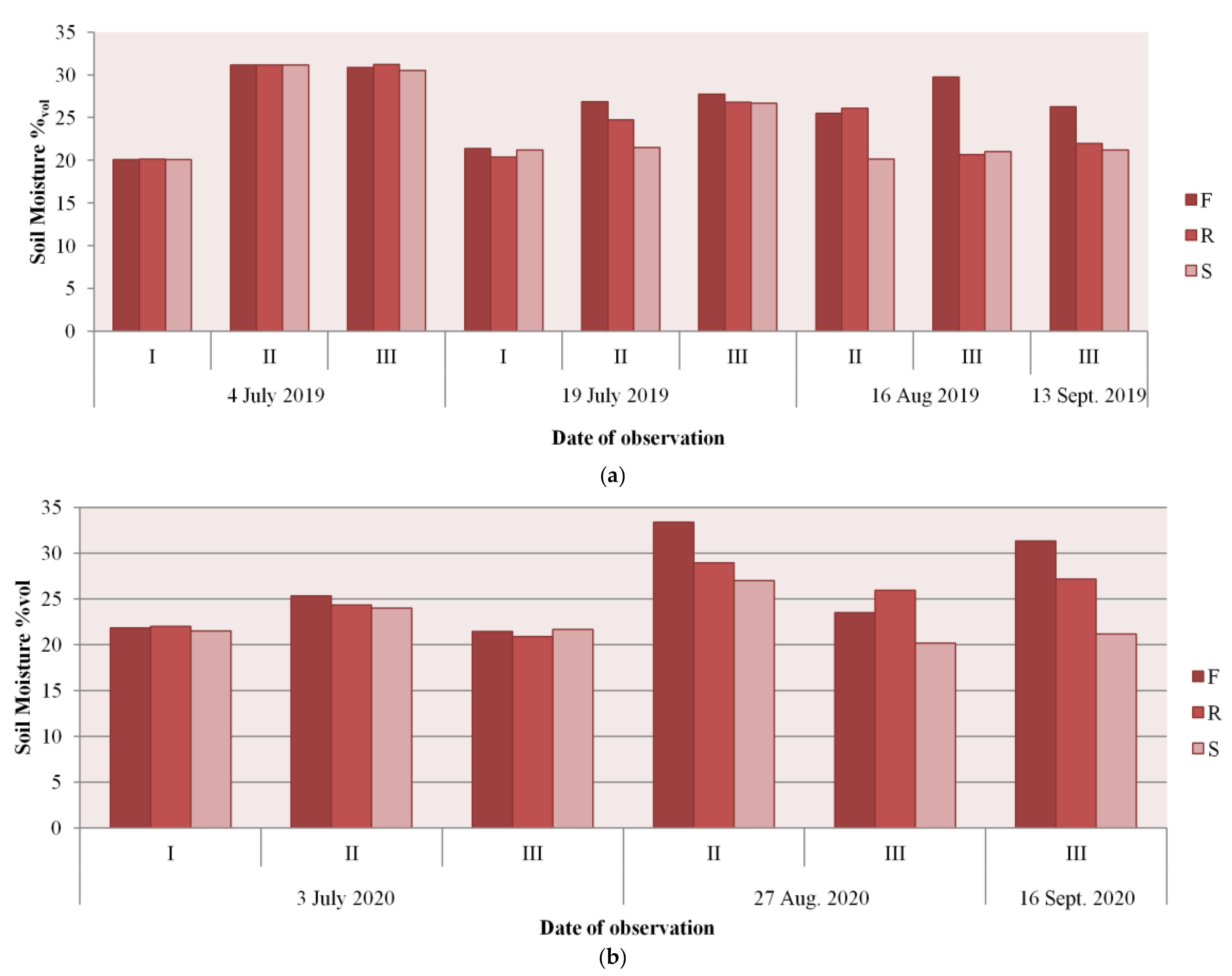
3.3. Soil Moisture
3.4. Leaf Area Index (LAI)
3.5. Vegetation Index Sensitivity to Irrigation Treatment
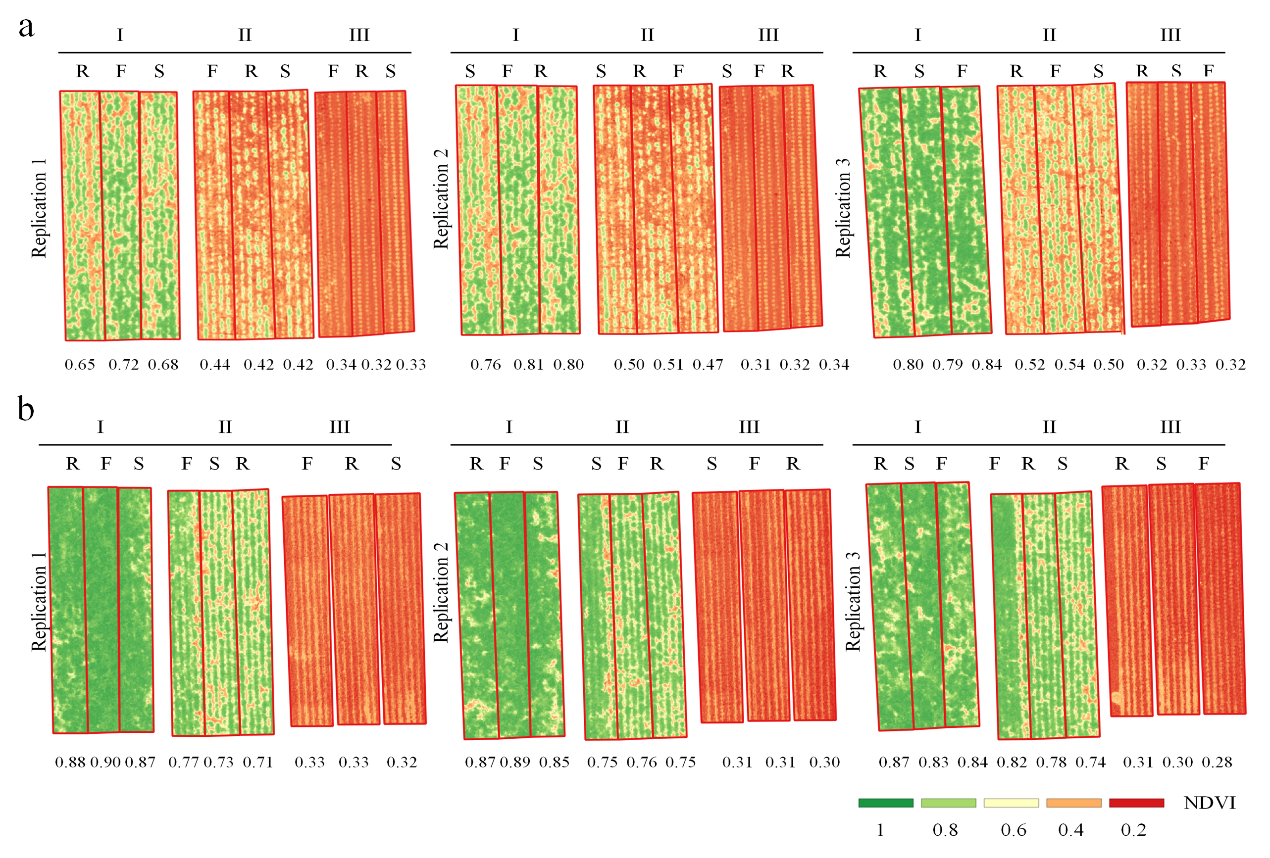
3.6. Mapping of Vegetation Indices for Spatial Presentation
3.7. Response of LAI, CC and VI to Sowing Period and Irrigation Treatment
3.8. Yield Prediction via Vegetation Indices
4. Discussion
5. Conclusions
Author Contributions
Funding
Data Availability Statement
Acknowledgments
Conflicts of Interest
References
- Forzieri, G.; Feyen, L.; Russo, S.; Vousdoukas, M.; Alfieri, L.; Outten, S.; Migliavacca, M.; Bianchi, A.; Rojas, R.; Cid, A. Multi-hazard assessment in Europe under climate change. Clim. Chang. 2016, 137, 105–119. [Google Scholar] [CrossRef] [Green Version]
- Stričević, R.; Srdjević, Z.; Lipovac, A.; Prodanović, S.; Petrović-Obradović, O.; Ćosić, M.; Djurović, N. Synergy of experts’ and farmers’ responses in climate-change adaptation planning in Serbia. Ecol. Indic. 2020, 116, 106481. [Google Scholar] [CrossRef]
- Fereres, E.; Soriano, M.A. Deficit irrigation for reducing agricultural water use. J. Exp. Bot. 2007, 58, 147–159. [Google Scholar] [CrossRef] [Green Version]
- Zhang, H.; Ma, L.; Douglas-Mankin, K.R.; Han, M.; Trout, T.J. Modeling maize production under growth stage-based deficit irrigation management with RZWQM2. Agric. Water Manag. 2021, 248, 106767. [Google Scholar] [CrossRef]
- Eyni-Nargeseh, H.; AghaAlikhani, M.; Shirani Rad, A.H.; Mokhtassi-Bidgoli, A.; Modarres Sanavy, S.A.M. Late season deficit irrigation for water-saving: Selection of rapeseed (Brassica napus) genotypes based on quantitative and qualitative features. Arch. Agron. Soil Sci. 2019, 66, 126–137. [Google Scholar] [CrossRef]
- Comas, L.H.; Trout, T.J.; DeJonge, K.C.; Zhang, H.; Gleason, S.M. Water productivity under strategic growth stage-based deficit irrigation in maize. Agric. Water Manag. 2019, 212, 433–440. [Google Scholar] [CrossRef]
- Ćosić, M.; Stričević, R.; Djurović, N.; Lipovac, A.; Bogdan, I.; Pavlović, M. Effects of irrigation regime and application of kaolin on canopy temperatures of sweet pepper and tomato. Sci. Hortic. (Amst.) 2018, 238, 23–31. [Google Scholar] [CrossRef]
- Bogale, A.; Nagle, M.; Latif, S.; Aguila, M.; Müller, J. Regulated deficit irrigation and partial root-zone drying irrigation impact bioactive compounds and antioxidant activity in two select tomato cultivars. Sci. Hortic. 2016, 213, 115–124. [Google Scholar] [CrossRef]
- Adu, M.O.; Yawson, D.O.; Armah, F.A.; Asare, P.A.; Frimpong, K.A. Meta-analysis of crop yields of full, deficit, and partial root-zone drying irrigation. Agric. Water Manag. 2018, 197, 79–90. [Google Scholar] [CrossRef]
- Al-Ghobari, H.M.; Dewidar, A.Z. Integrating deficit irrigation into surface and subsurface drip irrigation as a strategy to save water in arid regions. Agric. Water Manag. 2018, 209, 55–61. [Google Scholar] [CrossRef]
- Ayars, J.E.; Fulton, A.; Taylor, B. Subsurface drip irrigation in California—Here to stay? Agric. Water Manag. 2015, 157, 39–47. [Google Scholar] [CrossRef]
- Saleem, H.; Zaidi, S.J. Recent developments in the application of nanomaterials in agroecosystems. Nanomaterials 2020, 10, 2411. [Google Scholar] [CrossRef] [PubMed]
- Guerrero, A.; De Neve, S.; Mouazen, A.M. Data fusion approach for map-based variable-rate nitrogen fertilization in barley and wheat. Soil Tillage Res. 2021, 205, 104789. [Google Scholar] [CrossRef]
- Wu, D.; Xu, X.; Chen, Y.; Shao, H.; Sokolowski, E.; Mi, G. Effect of different drip fertigation methods on maize yield, nutrient and water productivity in two-soils in Northeast China. Agric. Water Manag. 2019, 213, 200–211. [Google Scholar] [CrossRef]
- Bateman, N.R.; Catchot, A.L.; Gore, J.; Cook, D.R.; Musser, F.R.; Irby, J.T. Effects of planting date for soybean growth, development, and yield in the Southern USA. Agronomy 2020, 10, 596. [Google Scholar] [CrossRef]
- Mirshekari, M.; Hosseini, N.M.; Amiri, R.; Zandvakili, O.R. Study the Effects of Planting Date and Low Irrigation. Rom. Agric. Res. 2012, 29, 189–199. [Google Scholar]
- Tunc, M.; Bicer, B.T.; Turk, Z. Cultivation Possibilities of Some Common Beans Varieties Under Second Crop Conditions. Cercet. Agron. Mold. 2020, 53, 144–151. [Google Scholar] [CrossRef]
- Zeleke, K.; Nendel, C. Growth and yield response of faba bean to soil moisture regimes and sowing dates: Field experiment and modelling study. Agric. Water Manag. 2019, 213, 1063–1077. [Google Scholar] [CrossRef]
- Delalieux, S.; Somers, B.; Hereijgers, S.; Verstraeten, W.W.; Keulemans, W.; Coppin, P. A near-infrared narrow-waveband ratio to determine Leaf Area Index in orchards. Remote Sens. Environ. 2008, 112, 3762–3772. [Google Scholar] [CrossRef]
- Agam, N.; Cohen, Y.; Berni, J.A.J.; Alchanatis, V.; Kool, D.; Dag, A.; Yermiyahu, U.; Ben-Gal, A. An insight to the performance of crop water stress index for olive trees. Agric. Water Manag. 2013, 118, 79–86. [Google Scholar] [CrossRef]
- Poirier-Pocovi, M.; Volder, A.; Bailey, B.N. Modeling of reference temperatures for calculating crop water stress indices from infrared thermography. Agric. Water Manag. 2020, 233, 106070. [Google Scholar] [CrossRef]
- Moriana, A.; Pérez-López, D.; Prieto, M.H.; Ramírez-Santa-Pau, M.; Pérez-Rodriguez, J.M. Midday stem water potential as a useful tool for estimating irrigation requirements in olive trees. Agric. Water Manag. 2012, 112, 43–54. [Google Scholar] [CrossRef]
- Lipan, L.; Issa-Issa, H.; Moriana, A.; Zurita, N.M.; Galindo, A.; Martín-Palomo, M.J.; Andreu, L.; Carbonell-Barrachina, Á.A.; Hernández, F.; Corell, M. Scheduling regulated deficit irrigation with leaf water potential of cherry tomato in greenhouse and its effect on fruit quality. Agriculture 2021, 11, 669. [Google Scholar] [CrossRef]
- Kirnak, H.; Irik, H.A.; Unlukara, A. Potential use of crop water stress index (CWSI) in irrigation scheduling of drip-irrigated seed pumpkin plants with different irrigation levels. Sci. Hortic. 2019, 256, 108608. [Google Scholar] [CrossRef]
- Weiss, M.; Jacob, F.; Duveiller, G. Remote Sensing for Agricultural Applications: A Meta-Review. Remote Sens. Environ. 2020, 236, 111402. [Google Scholar] [CrossRef]
- Liaghat, S.; Balasundram, S.K. A Review: The Role of Remote Sensing in Precision Agriculture. Am. J. Agric. Biol. Sci. 2010, 5, 50–55. [Google Scholar] [CrossRef] [Green Version]
- Shanmugapriya, P.; Rathika, S.; Ramesh, T.; Janaki, P. Applications of Remote Sensing in Agriculture—A Review. Int. J. Curr. Microbiol. Appl. Sci. 2019, 8, 2270–2283. [Google Scholar] [CrossRef]
- Droogers, P.; Immerzeel, W.W.; Lorite, I.J. Estimating Actual Irrigation Application by Remotely Sensed Evapotranspiration Observations. Agric. Water Manag. 2010, 97, 1351–1359. [Google Scholar] [CrossRef]
- Belmonte, A.C.; Jochum, A.M.; García, A.C.; Rodríguez, A.M.; Fuster, P.L. Irrigation Management from Space: Towards User-Friendly Products. Irrig. Drain. Syst. 2005, 19, 337–353. [Google Scholar] [CrossRef]
- Gowda, P.H.; Chávez, J.L.; Colaizzi, P.D.; Evett, S.R.; Howell, T.A.; Tolk, J.A. Remote Sensing Based Energy Balance Algorithms for Mapping ET: Current Status and Future Challenges. Trans. ASABE 2007, 50, 1639–1644. [Google Scholar]
- Mwinuka, P.R.; Mbilinyi, B.P.; Mbungu, W.B.; Mourice, S.K.; Mahoo, H.F.; Schmitter, P. The feasibility of hand-held thermal and UAV-based multispectral imaging for canopy water status assessment and yield prediction of irrigated African eggplant (Solanum aethopicum L). Agric. Water Manag. 2021, 245, 106584. [Google Scholar] [CrossRef]
- Yu, N.; Li, L.; Schmitz, N.; Tian, L.F.; Greenberg, J.A.; Diers, B.W. Development of methods to improve soybean yield estimation and predict plant maturity with an unmanned aerial vehicle based platform. Remote Sens. Environ. 2016, 187, 91–101. [Google Scholar] [CrossRef]
- Li, W.; Niu, Z.; Chen, H.; Li, D.; Wu, M.; Zhao, W. Remote estimation of canopy height and aboveground biomass of maize using high-resolution stereo images from a low-cost unmanned aerial vehicle system. Ecol. Indic. 2016, 67, 637–648. [Google Scholar] [CrossRef]
- Tunca, E.; Köksal, E.S.; Çetin, S.; Ekiz, N.M.; Balde, H. Yield and leaf area index estimations for sunflower plants using unmanned aerial vehicle images. Environ. Monit. Assess. 2018, 190, 682. [Google Scholar] [CrossRef]
- Gonzalez-Dugo, V.; Zarco-Tejada, P.; Nicolás, E.; Nortes, P.A.; Alarcón, J.J.; Intrigliolo, D.S.; Fereres, E. Using high resolution UAV thermal imagery to assess the variability in the water status of five fruit tree species within a commercial orchard. Precis. Agric. 2013, 14, 660–678. [Google Scholar] [CrossRef]
- Virnodkar, S.S.; Pachghare, V.K.; Patil, V.C.; Jha, S.K. Remote Sensing and Machine Learning for Crop Water Stress Determination in Various Crops: A Critical Review; Springer: New York, NY, USA, 2020; Volume 21, ISBN 0123456789. [Google Scholar]
- Nemeskéri, E.; Molnár, K.; Helyes, L. Relationships of spectral traits with yield and nutritional quality of snap beans (Phaseolus vulgaris L.) in dry seasons. Arch. Agron. Soil Sci. 2018, 64, 1222–1239. [Google Scholar] [CrossRef]
- Hong, M.; Bremer, D.J.; van der Merwe, D. Using Small Unmanned Aircraft Systems for Early Detection of Drought Stress in Turfgrass. Crop Sci. 2019, 59, 2829–2844. [Google Scholar] [CrossRef]
- Stone, K.C.; Bauer, P.J.; Sigua, G.C. Irrigation management using an expert system, soil water potentials, and vegetative indices for spatial applications. Trans. ASABE 2016, 59, 941–948. [Google Scholar] [CrossRef]
- Zhou, J.; Khot, L.R.; Boydston, R.A.; Miklas, P.N.; Porter, L. Low altitude remote sensing technologies for crop stress monitoring: A case study on spatial and temporal monitoring of irrigated pinto bean. Precis. Agric. 2018, 19, 555–569. [Google Scholar] [CrossRef]
- Köksal, E.S.; Erdem, C.; Taşan, M.; Temizel, K.E. Developing New Hyperspectral Vegetation Indexes Sensitive to Yield and Evapotranspiration of Dry Beans. Turkish J. Agric. For. 2021, 45, 743–749. [Google Scholar] [CrossRef]
- Sankaran, S.; Zhou, J.; Khot, L.R.; Trapp, J.J.; Mndolwa, E.; Miklas, P.N. High-throughput field phenotyping in dry bean using small unmanned aerial vehicle based multispectral imagery. Comput. Electron. Agric. 2018, 151, 84–92. [Google Scholar] [CrossRef]
- Rai, A.; Sharma, V.; Heitholt, J. Dry bean [phaseolus vulgaris L.] growth and yield response to variable irrigation in the arid to semi-arid climate. Sustainability 2020, 12, 3851. [Google Scholar] [CrossRef]
- Ranjan, R.; Chandel, A.K.; Khot, L.R.; Bahlol, H.Y.; Zhou, J.; Boydston, R.A.; Miklas, P.N. Irrigated pinto bean crop stress and yield assessment using ground based low altitude remote sensing technology. Inf. Process. Agric. 2019, 6, 502–514. [Google Scholar] [CrossRef]
- FAOSTAT: FAO Statistical Databases (Food and Agriculture Organization of the United Nations). 2018. Available online: https://www.fao.org/faostat/en/#home (accessed on 14 April 2018).
- Škorić, A.; Filipovski, G.; Čirić, M. Soil Classification of Yugoslavia, Academy of Sciences and Artists of Bosnia and Herzegovina. In Special Issue, Book LXXVII, Sarajevo; Academy of Sciences and Arts of Bosnia and Herzegovina: Sarajevo, Bosnia and Herzegovina, 1985. (In Serbian) [Google Scholar]
- USDA. Kellogg Soil Survey Laboratory Methods Manual; Soil Survey Investigations Report No. 42, Version 5.0; Burt, R., Staff, S.S., Eds.; U.S. Department of Agriculture, Natural Resources Conservation Service: Washington, DC, USA, 2014.
- Allen, R.G.; Pereira, L.S.; Raes, D.; Smith, M. Crop evapotranspiration: Guidelines for computing crop water requirements. In FAO Irrigation and Drainage Paper 56; UN-FAO: Rome, Italy, 1998. [Google Scholar]
- Ustuner, M.; Sanli, F.B.; Abdikan, S.; Esetlili, M.T.; Kurucu, Y. Crop type classification using vegetation indices of rapideye imagery. Int. Arch. Photogramm. Remote Sens. SpatialInf. Sci. 2014, 40, 195. [Google Scholar] [CrossRef] [Green Version]
- Haboudane, D.; Miller, J.R.; Pattey, E.; Zarco-Tejada, P.J.; Strachan, I.B. Hyperspectral vegetation indices and novel algorithms for predicting green LAI of crop canopies: Modeling and validation in the context of precision agriculture. Remote Sens. Environ. 2004, 90, 337–352. [Google Scholar] [CrossRef]
- Gitelson, A.; Merzlyak, M.N. Quantitative estimation of chlorophyll-a using reflectance spectra: Experiments with autumn chestnut and maple leaves. J. Photochem. Photobiol. B Biol. 1994, 22, 247–252. [Google Scholar] [CrossRef]
- Omer, G.; Mutanga, O.; Abdel-Rahman, E.M.; Peerbhay, K.; Adam, E. Mapping leaf nitrogen and carbon concentrations of intact and fragmented indigenous forest ecosystems using empirical modeling techniques and WorldView-2 data. ISPRS J. Photogramm. Remote Sens. 2017, 131, 26–39. [Google Scholar] [CrossRef]
- Zou, X.; Mottus, M. Sensitivity of common vegetation indices to the canopy structure of field crops. Remote Sens. 2017, 9, 994. [Google Scholar] [CrossRef] [Green Version]
- SAS Statistical Package; SAS Version 9.1.3; SAS Institute Inc.: Cary, NC, USA, 2007.
- Karimzadeh, H.; Nezami, A.; Kafi, M. Responses of two common bean (Phaseolus vulgaris L.) genotypes to deficit irrigation. Agric. Water Manag. 2019, 213, 270–279. [Google Scholar] [CrossRef]
- Srivastava, R.K.; Panda, R.K.; Chakraborty, A.; Halder, D. Quantitative estimation of water use efficiency and evapotranspiration under varying nitrogen levels and sowing dates for rainfed and irrigated maize. Theor. Appl. Climatol. 2020, 139, 1385–1400. [Google Scholar] [CrossRef]
- Lipovac, A.; Stričević, R.; Ćosić, M.; Djurović, N. Productive and non-productive use of water of common bean under full and deficit irrigation. Acta Hortic. 2022, 1335, 635–641. [Google Scholar] [CrossRef]
- Lillesand, T.M.; Kiefer, R.W.; Chipman, J.W. Remote Sensing and Image Interpretation; John Wiley & Sons: Hoboken, NJ, USA, 2008. [Google Scholar]
- Vasić, M.; Milić, S.; Pejić, B.; Gvozdanović-Varga, J.; Maksimović, L.; Bošnjak, D. The possibility of after production of beans (Phaseolus vulgaris L) in the agro-ecological conditions of Vojvodina. J. Inst. Field Veg. Crops 2007, 43, 283–291. [Google Scholar]
- Bréda, N.J.J. Ground-based measurements of leaf area index: A review of methods, instruments and current controversies. J. Exp. Bot. 2003, 54, 2403–2417. [Google Scholar] [CrossRef] [Green Version]
- Heshmat, K.; Asgari Lajayer, B.; Shakiba, M.R.; Astatkie, T. Assessment of physiological traits of common bean cultivars in response to water stress and molybdenum levels. J. Plant Nutr. 2021, 44, 366–372. [Google Scholar] [CrossRef]
- Boydston, R.A.; Porter, L.D.; Chaves-Cordoba, B.; Khot, L.R.; Miklas, P.N. The impact of tillage on pinto bean cultivar response to drought induced by deficit irrigation. Soil Tillage Res. 2018, 180, 63–72. [Google Scholar] [CrossRef]
- Duchemin, B.; Hadria, R.; Erraki, S.; Boulet, G.; Maisongrande, P.; Chehbouni, A.; Escadafal, R.; Ezzahar, J.; Hoedjes, J.C.B.; Kharrou, M.H.; et al. Monitoring wheat phenology and irrigation in Central Morocco: On the use of relationships between evapotranspiration, crops coefficients, leaf area index and remotely-sensed vegetation indices. Agric. Water Manag. 2006, 79, 1–27. [Google Scholar] [CrossRef]
- Toureiro, C.; Serralheiro, R.; Shahidian, S.; Sousa, A. Irrigation management with remote sensing: Evaluating irrigation requirement for maize under Mediterranean climate condition. Agric. Water Manag. 2017, 184, 211–220. [Google Scholar] [CrossRef]
- Zhang, H.; Oweis, T. Water-yield relations and optimal irrigation scheduling of wheat in the Mediterranean region. Agric. Water Manag. 1999, 38, 195–211. [Google Scholar] [CrossRef]
- Rinaldi, M.; Castrignanò, A.; De Benedetto, D.; Sollitto, D.; Ruggieri, S.; Garofalo, P.; Santoro, F.; Figorito, B.; Gualano, S.; Tamborrino, R. Discrimination of tomato plants under different irrigation regimes: Analysis of hyperspectral sensor data. Environmetrics 2014, 26, 77–88. [Google Scholar] [CrossRef]
- Monterroso, V.A.; Wien, H.C. Flower and Pod Abscission Due to Heat Stress in Beans. J. Am. Soc. Hortic. Sci. 2019, 115, 631–634. [Google Scholar] [CrossRef]
- Konsens, I.; Ofir, M.; Kigel, J. The Effect of Temperature on the Production and Abscission of Flowers and Pods in Snap Bean (Phaseolus vulgaris L.). Ann. Bot. 1991, 67, 391–399. [Google Scholar] [CrossRef]
- Herrera, M.D.; Reynoso-Camacho, R.; Melero-Meraz, V.; Guzmán-Maldonado, S.H.; Acosta-Gallegos, J.A. Impact of soil moisture on common bean (Phaseolus vulgaris L.) phytochemicals. J. Food Compos. Anal. 2021, 99, 103883. [Google Scholar] [CrossRef]
- Hoffmann, H.; Jensen, R.; Thomsen, A.; Nieto, H.; Rasmussen, J.; Friborg, T. Crop water stress maps for an entire growing season from visible and thermal UAV imagery. Biogeosciences 2016, 13, 6545–6563. [Google Scholar] [CrossRef]
- Lelong, C.C.D.; Burger, P.; Jubelin, G.; Roux, B.; Labbé, S.; Baret, F. Assessment of unmanned aerial vehicles imagery for quantitative monitoring of wheat crop in small plots. Sensors 2008, 8, 3557–3585. [Google Scholar] [CrossRef]
- Spitkó, T.; Nagy, Z.; Zsubori, Z.T.; Szőke, C.; Berzy, T.; Pintér, J.; Marton, C.L. Connection between normalized difference vegetation index and yield in maize. Plant Soil Environ. 2016, 62, 293–298. [Google Scholar] [CrossRef]
- Da Silva, E.E.; Rojo Baio, F.H.; Ribeiro Teodoro, L.P.; da Silva Junior, C.A.; Borges, R.S.; Teodoro, P.E. UAV-multispectral and vegetation indices in soybean grain yield prediction based on in situ observation. Remote Sens. Appl. Soc. Environ. 2020, 18, 100318. [Google Scholar] [CrossRef]
- Hunt, E.R.; Rondon, S.I. Detection of potato beetle damage using remote sensing from small unmanned aircraft systems. J. Appl. Remote Sens. 2017, 11, 026013. [Google Scholar] [CrossRef] [Green Version]
- Veysi, S.; Naseri, A.A.; Hamzeh, S.; Bartholomeus, H. A satellite based crop water stress index for irrigation scheduling in sugarcane fields. Agric. Water Manag. 2017, 189, 70–86. [Google Scholar] [CrossRef]
- Tenreiro, T.R.; García-Vila, M.; Gómez, J.A.; Jiménez-Berni, J.A.; Fereres, E. Using NDVI for the assessment of canopy cover in agricultural crops within modelling research. Comput. Electron. Agric. 2021, 182, 106038. [Google Scholar] [CrossRef]
- Trout, T.J.; Johnson, L.F.; Gartung, J. Remote sensing of canopy cover in horticultural crops. HortScience 2008, 43, 333–337. [Google Scholar] [CrossRef] [Green Version]
- Gitelson, A.A. Remote estimation of crop fractional vegetation cover: The use of noise equivalent as an indicator of performance of vegetation indices. Int. J. Remote Sens. 2013, 34, 6054–6066. [Google Scholar] [CrossRef]


| Year | Irrigation Treatment/Sowing Period | I | II | III | |||
|---|---|---|---|---|---|---|---|
| Irrigation Depth (mm) | Irrigation Events | Irrigation Depth (mm) | Irrigation Events | Irrigation Depth (mm) | Irrigation Events | ||
| 2019 | F | 0 | 0 | 150 | 9 | 249 | 15 |
| R | 0 | 0 | 117 | 7 | 180 | 11 | |
| S | 0 | 0 | 84 | 5 | 129 | 8 | |
| 2020 | F | 228 | 14 | 141 | 9 | 200 | 13 |
| R | 162 | 10 | 90 | 6 | 144 | 9 | |
| S | 126 | 8 | 75 | 5 | 111 | 7 | |
| Band Number | Band Name | Spatial Resolution (cm) | Wavelength Range (Micrometer) | Central Wavelength (Micrometer) |
|---|---|---|---|---|
| 1 | Blue | 3.7 | 0.465–0.485 | 0.475 |
| 2 | Green | 0.550–0.570 | 0.560 | |
| 3 | Red | 0.663–0.673 | 0.668 | |
| 4 | Red edge | 0.712–0.722 | 0.717 | |
| 5 | Near infrared | 0.820–0.860 | 0.840 |
| Year 1 | Year 2 |
|---|---|
| 4 July 2019 | 3 July 2020 |
| 19 July 2019 | 27 August 2020 |
| 16 August 2019 | 16 September 2020 |
| 13 September 2019 |
| Index | Equation | Reference |
|---|---|---|
| Normalized Difference Vegetation Index | [49] | |
| Modified Chlorophyll Absorption in Reflectance Index | [50] | |
| Normalized Difference Red Edge | [51] | |
| Green Normalized Difference Vegetation Index | [52] | |
| Optimized Soil Adjusted Vegetation Index | [53] |
| Irrigation | F | R | S | |||||||||
|---|---|---|---|---|---|---|---|---|---|---|---|---|
| Variable | CC | LAI | T | Sm | CC | LAI | T | Sm | CC | LAI | T | Sm |
| NDVI | 0.94 ** | 0.79 ** | 0.71 ** | −0.29 ns | 0.95 ** | 0.79 ** | 0.67 ** | −0.48 ** | 0.94 ** | 0.74 ** | 0.62 ** | −0.61 ** |
| MCARI11 | 0.83 ** | 0.71 ** | 0.78 ** | −0.31 * | 0.84 ** | 0.68 ** | 0.59 ** | −0.53 ** | 0.83 ** | 0.56 ** | 0.52 ** | −0.60 ** |
| NDRE | 0.71 ** | 0.57 ** | 0.53 ** | −0.34 * | 0.71 ** | 0.53 ** | 0.44 ** | −0.59 ** | 0.67 ** | 0.39 ** | 0.38 ** | −0.60 ** |
| GNDVI | 0.66 ** | 0.51 ** | 0.55 ** | −0.34 * | 0.66 * | 0.49 ** | 0.45 ** | −0.46 ** | 0.64 ** | 0.40 ** | 0.41 ** | −0.51 ** |
| OSAVI | 0.45 ** | 0.55 ** | 0.36 * | −0.42 ** | 0.41 ** | 0.47 ** | 0.37 * | −0.49 ** | 0.38 * | 0.45 ** | 0.39 ** | −0.70 ** |
| Treatment 2019 | CC | Yield | LAI | NDVI | MCARI11 | GNDVI | OSAVI | NDRE |
|---|---|---|---|---|---|---|---|---|
| I-F | ns | ns | ns | ns | ns | ns | ns | ns |
| I-R | ns | ns | ns | ns | ns | ns | ns | ns |
| I-S | ns | ns | ns | ns | ns | ns | ns | ns |
| II-F | ns | ns | ns | ns | ns | ns | ns | ns |
| II-R | ns | * | * | ns | ns | ns | ns | ns |
| II-S | * | * | * | * | * | ns | ns | ns |
| III-F | ns | ns | ns | ns | ns | ns | ns | ns |
| III-R | ns | ns | ns | ns | ns | ns | ns | ns |
| III-S | * | * | * | * | * | * | ns | ns |
| 2020 | ||||||||
| I-F | ns | ns | ns | ns | ns | ns | ns | ns |
| I-R | * | ns | ns | ns | ns | ns | ns | ns |
| I-S | * | ** | * | * | * | * | ns | ns |
| II-F | ns | ns | ns | ns | ns | ns | ns | ns |
| II-R | ns | ** | * | ns | ns | ns | ns | ns |
| II-S | * | ** | * | * | * | * | ns | ns |
| III-F | ns | ns | ns | ns | ns | ns | ns | ns |
| III-R | ns | ** | * | ns | ns | ns | ns | ns |
| III-S | * | ** | * | * | * | * | ns | ns |
| Treatment | NDVI | MCARI11 | GNDVI | |||||||||
|---|---|---|---|---|---|---|---|---|---|---|---|---|
| Mean | SD | Model | r2 | Mean | SD | Model | r2 | Mean | SD | Model | r2 | |
| I-F | 0.79 | 0.07 | ns | 0.57 | 0.08 | 0.92 | 0.06 | ns | ||||
| I-R | 0.77 | 0.16 | ns | 0.54 | 0.09 | 0.90 | 0.05 | ns | ||||
| I-S | 0.67 | 0.3 | ns | 0.53 | 0.01 | 0.91 | 0.02 | ns | ||||
| II-F | 0.67 | 0.09 | ns | 0.48 | 0.09 | 0.81 | 0.04 | ns | ||||
| II-R | 0.63 | 0.04 | ns | 0.45 | 0.3 | 0.75 | 0.03 | ns | ||||
| II-S | 0.56 | 0.11 | y = 794.91x + 3910 | 0.42 | 0.39 | 0.1 | y = 379.89x + 3716 | 0.25 | 0.67 | 0.14 | ns | |
| III-F | 0.63 | 0.04 | ns | 0.55 | 0.04 | ns | 0.82 | 0.04 | ns | |||
| III-R | 0.61 | 0.08 | ns | 0.54 | 0.08 | ns | 0.77 | 0.05 | ns | |||
| III-S | 0.51 | 0.10 | y = 791.24x + 3655 | 0.57 | 0.42 | 0.01 | y = 320.14x + 3501 | 0.20 | 0.65 | 0.12 | y = 472.18x + 3543 | 0.32 |
| Treatment | NDVI | MCARI11 | GNDVI | ||||||
|---|---|---|---|---|---|---|---|---|---|
| Yield a | r2 | p | Yield | r2 | P | Yield | r2 | p | |
| I-F | ns | ns | ns | ns | ns | ns | ns | ns | ns |
| I-R | ns | ns | ns | ns | ns | ns | ns | ns | ns |
| I-S | ns | ns | ns | ns | ns | ns | ns | ns | ns |
| II-F | ns | ns | ns | ns | ns | ns | ns | ns | ns |
| II-R | ns | ns | ns | ns | ns | ns | ns | ns | ns |
| II-S | 4.01 | 0.65 | 0.01 | 4.28 | 0.70 | 0.012 | ns | ns | ns |
| III-F | ns | ns | ns | ns | ns | ns | ns | ns | ns |
| III-R | ns | ns | ns | ns | ns | ns | ns | ns | ns |
| III-S | 3.54 | 0.012 | 0.02 | 3.62 | 0.020 | 0.018 | 3.7 | 0.14 | 0.35 |
Publisher’s Note: MDPI stays neutral with regard to jurisdictional claims in published maps and institutional affiliations. |
© 2022 by the authors. Licensee MDPI, Basel, Switzerland. This article is an open access article distributed under the terms and conditions of the Creative Commons Attribution (CC BY) license (https://creativecommons.org/licenses/by/4.0/).
Share and Cite
Lipovac, A.; Bezdan, A.; Moravčević, D.; Djurović, N.; Ćosić, M.; Benka, P.; Stričević, R. Correlation between Ground Measurements and UAV Sensed Vegetation Indices for Yield Prediction of Common Bean Grown under Different Irrigation Treatments and Sowing Periods. Water 2022, 14, 3786. https://doi.org/10.3390/w14223786
Lipovac A, Bezdan A, Moravčević D, Djurović N, Ćosić M, Benka P, Stričević R. Correlation between Ground Measurements and UAV Sensed Vegetation Indices for Yield Prediction of Common Bean Grown under Different Irrigation Treatments and Sowing Periods. Water. 2022; 14(22):3786. https://doi.org/10.3390/w14223786
Chicago/Turabian StyleLipovac, Aleksa, Atila Bezdan, Djordje Moravčević, Nevenka Djurović, Marija Ćosić, Pavel Benka, and Ružica Stričević. 2022. "Correlation between Ground Measurements and UAV Sensed Vegetation Indices for Yield Prediction of Common Bean Grown under Different Irrigation Treatments and Sowing Periods" Water 14, no. 22: 3786. https://doi.org/10.3390/w14223786