Abstract
Rivers are dynamic geological agents on the earth which transport the weathered materials of the continent to the sea. Estimation of suspended sediment yield (SSY) is essential for management, planning, and designing in any river basin system. Estimation of SSY is critical due to its complex nonlinear processes, which are not captured by conventional regression methods. Rainfall, temperature, water discharge, SSY, rock type, relief, and catchment area data of 11 gauging stations were utilized to develop robust artificial intelligence (AI), similar to an artificial-neural-network (ANN)-based model for SSY prediction. The developed highly generalized global single ANN model using a large amount of data was applied at individual gauging stations for SSY prediction in the Mahanadi River basin, which is one of India’s largest peninsular rivers. It appeared that the proposed ANN model had the lowest root-mean-squared error (0.0089) and mean absolute error (0.0029) along with the highest coefficient of correlation (0.867) values among all comparative models (sediment rating curve and multiple linear regression). The ANN provided the best accuracy at Tikarapara among all stations. The ANN model was the most suitable substitute over other comparative models for SSY prediction. It was also noticed that the developed ANN model using the combined data of eleven stations performed better at Tikarapara than the other ANN which was developed using data from Tikarapara only. These approaches are suggested for SSY prediction in river basin systems due to their ease of implementation and better performance.
Keywords:
SSY; rainfall; water discharge; ANN; temperature; multiple linear regression; sediment rating curve 1. Introduction
The complex nonlinear process of sediment flow in a river basin involves the interaction of hydro-geo-climatical components with time and spatial variation. Rivers carry a huge amount of sediment load that flow through a variety of active tectonic zones, climates, and highly erodible materials [1]. Modeling of sediment transport in a river is critical for managing hydraulic structures, which is the primary issue in accessing the world’s surface water system [2,3]. The proper assessment of SSY is required to understand sediment transport in water resource management, territorial risks, water system quality, land use, pollution control, and engineering structure damage caused by the morphological development of the river bed [4,5].
Unfortunately, failure to pay attention to the appropriate SSY measurements and computations could lead to a waste of energy, funds, people, and time [4,6]. The interaction of several complex processes makes it difficult to estimate SSY with high accuracy using conventional methods, such as the SRC and MLR methods. These methods cannot handle the complicated non-stationarity and nonlinearity of SSY. The ANN is one of the most popular artificial intelligence (AI) techniques and is most suited for the prediction of complex nonlinearity and dynamic systems in water resources due to its cost-effectiveness, simplicity, and few data requirements for prediction [7,8,9]. The main advantage of the black box ANN technique over traditional methods is the complexity of underlying processes which are not recognized to be explicitly described in mathematical form. The ANN has been used by many researchers in hydrological research including runoff or flow predictions [10,11,12,13], estimation of runoff hydrograph parameters [14], estimation of water quality parameters [15,16], reservoir operation optimization [17], water quality management [18] and non-point source contamination [19]. Various studies have extensively used intelligent ANN techniques to estimate SSY in river basin systems [20,21,22,23,24,25,26,27,28,29].
An ANN model was proposed by Zhu et al. [20] to simulate the monthly flux of suspended sediment in the Long Chuan Jiang River in the Upper Yangtze Catchments, China, using average temperature, rainfall, flow discharge, and rainfall intensity as inputs. The ANN model’s results demonstrated that it is capable of simulating suspended sediment flux with acceptable accuracy on a monthly basis by relating appropriate input parameters and their co-relation to the prior month (lagging effect) on the suspended sediment flux. Furthermore, the ANN was found to be a suitable technique in comparison to traditional regression models (MLR and SRC) and capable of estimating extremely high or low values of suspended sediment flux. Rajaee et al. [21] developed ANN, SRC, and MLR models to estimate suspended sediment concentrations in the little black and salt rivers of the United Kingdom. The results revealed that the ANN model performed better than the MLR and SRC. It was also revealed that the ANN model can estimate cumulative sediment. Melesse et al. [22] estimated suspended sediment load using an ANN model and daily and weekly hydro-climatological data (precipitation, water discharge, antecedent water discharge, and antecedent suspended sediment load). The MLR, multiple non-linear regression, and autoregressive moving average (ARMA) methods were used to compare the ANN model. The ANN model outperformed the comparison models. A prediction model for sediment and runoff yield was proposed by Sharma et al. [24] using ANN and regressions in the Nepal watershed Kankai Mai. The ANN provided a dominant result over the regression method.
The current research demonstrates the capability and utility of the ANN model which is one of the most suitable AI techniques for simulating complex nonlinear processes of SSY in the Mahanadi River basin (MRB). In the MRB, India, many quantitative and ANN techniques have been utilized to estimate RF, runoff, WD, and flood risk [30,31,32]. There have not been many SSY prediction studies in the MRB. Yadav et al. [25] developed the gradient descending adaptive (GDA) learning rate, Levenberg–Marquardt (LM)-based ANN, and classical models using T, WD, and RF components as input data to predict SSY at Tikarapara station in MRB. It was reported that the GDA-learning-rate-based ANN model, which was previously used by Kisi [4] in the estimation of SSY in Valenciano Quebrada Blanca and Rio stations, USA produced inferior results to the LM-based ANN model. It is also found that the ANN model was more efficient and it outperformed conventional regression-based models in terms of accuracy but it was limited to Tikarapara station in MRB only. Samantaray and Ghose [33] developed an ANN model for SSY estimation and found it had satisfactory performance, but this was limited to the Salebhata gauging station in MRB only. Yadav et al. [24] also developed artificial intelligence (AI) models which are based on hydro climatical data, such as water discharge (WD), rainfall (RF), and temperature (T) as inputs for SSY prediction at a single Tikarapara station in the MRB. It was found that WD, RF, and T input data provided the best results with different input parameter selection. Furthermore, it has been noted that the ANN model produced superior results compared to conventional-regression-analysis-based models. Yadav [26] also developed AI-based models at a single Tikarapara gauge station using WD, RF, T, rock type (RT), relief ®, and catchment area (CA) as inputs. No attempt has been made to predict SSY at multiple gauge stations using a single model in the entire MRB using the ANN techniques with temporal data (WD, RF, and T) and spatial data (RT, R, and CA). Thus, in this study, a single generalized ANN model was developed using the combined data of 11 gauge stations to estimate SSY at each station of the 11 gauging stations of the entire MRB using the hydro-geo-climatical WD, RF, T, RT, R, and CA data as major controlling factors of SSY. The parameters for some AI methods are selected by a trial-and-error method to obtain a reasonably good result. However, this approach takes a significantly large amount of computational time to obtain the parameter value, and is also not guaranteed to be the optimal or near-optimal solution to the problems. In this study, the parameters for the ANN model were selected by the grid search technique to obtain a passably good result. After the development of a reliable ANN-based prediction model, the performance of the model was examined with the same test dataset. The results demonstrated that the proposed ANN-based model performed satisfactorily and had a greater capacity for generalization than other comparative MLR and SRC methods for SSY prediction. Moreover, the ANN model, which is developed using the combined data of 11 stations, provided better results at Tikarapara than the ANN models using the data of Tikarapara station only (ANN-1) and had more generalization capability. The ANN-1 model is developed using the RF, WD, T, RT, CA, and R of a single Tikarapara station only using the same method as the ANN model which is developed combined data of 11 gauging stations. Among all gauging stations, the proposed ANN prediction model provided the best accuracy at Tikarapara gauging station. It could be because Tikarapara is situated at the far downstream end of the MRB basin before meeting with the Bay of Bengal which has the maximum CA, RF, WD, and SSY among all the gauging stations. Many researchers have developed artificial intelligence (AI) models to predict sediment load by considering a set of temporal parameters, such as WD, RF, and T, for a specific geographical location. The ANN model prepared based on the data of 11 gauging stations performed better than the ANN-1 model which was developed based on the data of individual stations (Tikarapara) and has a greater generalization capability than the individual models of different gauging stations. The MRB case study focuses on the development of a highly generalized global single AI model using a huge amount of temporal as well as spatial data from 11 gauging stations and applied it at individual stations for the prediction of SSY in river systems which is our unique contribution.
The proposed ANN prediction model of SSY which is hydro-geo-climatic-variable-dependent is very helpful for planners and managers of water resources to have a good understanding of the problems and find alternative solutions to handle problems in the future. If a measurement of SSY is not available, then this proposed ANN-based modeling approach can be recommended for the prediction of SSY in river basin systems due to its comparatively superior performance and its ease of implementation.
2. Study Region
The Mahanadi River basin (MRB) was chosen in this study for SSY prediction. It is the fourth-largest river basin in India, with a total CA of 141,589 km2, accounting for 4.3% of India’s total geographical area [34]. The MRB is located between latitudes 19°20′ and 23°35′ north and between longitudes 80°30′ and 86°50′ east. At an altitude of roughly 442 m above sea level, the Mahanadi River starts in Raipur, Chhattisgarh, halfway between Pharsiya Village and Nagri Town. A total of 53 % of the river’s CA contribution is made in Chhattisgarh, 46% in Odisha, and the remaining amounts are split evenly between Maharashtra and Jharkhand [34,35]. According to the current sediment load, in terms of capacity to cause flooding and water potential, the MRB is ranked second among the Indian peninsular rivers [36,37]. From 1971 to 2004, the mean annual RF in the MRB basin ranged between twelve hundred and fourteen hundred mm [36]. According to daily statistics for the years 1969 to 2004, the two coldest months of the year are January and December with the lowest temperatures of 12°C, and the two warmest months of the year are May and April with the highest temperatures of 39°C to 40°C [36]. The river’s basin area contribution for the years 2005–2006 was 54.27% under agricultural land cover, 5.24% under wasteland, 32.74% under forest cover, 3.30% under built-up land, and 4.45% under aquatic bodies [36]. The Chilika Lake and Hirakud reservoir are two large sources of water in the MRB. A geographical location map of the MRB including gauging sites is shown in Figure 1. The different lithologies found in the basin area include 5% coastal alluvium, 7% khondalite, 15% charnockite, 17% shale and Lower Gondwana limestone, and 22% shale and Upper Gondwana sandstone [38]. Among the 11 measuring stations, Tikarapara has the lowest elevation, while Baronda has the highest. The maximum CA value (124,450 km2) is found at Tikarapara, which lies on the downward side of the MRB before it meets the Bay of Bengal, while the lowest CA value (2210 km2) is found in Andhiyarakhore, which lies in the upper part of the MRB. Table 1 summarizes the subbasin and tributary descriptions of the MRB. The highest CA is found in the Seonath tributary, while the lowest is found in the Jonk. There is an abundance of literature that has provided a full description of the MRB [24,25,29,37].
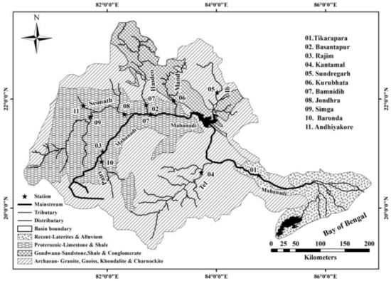
Figure 1.
Location map of the MRB with eleven gauging stations.

Table 1.
Sub-basins and tributaries of the MRB with catchment areas.
3. Methodology
A specific kind of AI model is the ANN which is widely used. The ANN is capable of learning complex nonlinear correlations among variables. The ANN’s goal is to create pattern recognition as a learning approach so that it can learn from data and predict output [39,40,41]. The ANN may represent any arbitrarily complicated nonlinear process that associates SSY with real-time hydro-geo-climatic factors [42]. The ANN is a flexible mathematical framework that resembles the biological brain in many ways [43]. It is based on the concept of a biological brain and the neurological system that surrounds it [43]. ANN-based models have grown in popularity for the modeling of hydrological processes over the last two decades [44]. The ANN is capable of handling high-speed and high-accuracy simulations of hydrological processes. There are certain ANNs, such as the general regression neural network and the feedforward backpropagation neural network (FBNN) [45]. The FBNN is the most commonly employed since it is computationally efficient for multi-layer perceptual training (MLP). The major aim of this research is to assess the effectiveness of ANN in estimating SSY in the MRB using 20 years of monthly temporal data (RF, T, SSY, and WD) as well as spatial data (RT, R, and CA) from 1990 to 2010. To develop a robust model, data are normalized between 0 and 1 and separated into three categories: 15% validation, 15% testing, and 70% training. The primary goal of the data normalization is used to remove the various ranges and dimensions of the parameters in the data set. The normalization was performed for all inputs and output variables used in this study. The normalization process of the data in the range of a and b is conducted using the following equations:
where is the ith original value, is the normalized value of , is the maximum value and is the minimum value of the data set. All of the output and input variables employed in this study were normalized between 0 and 1. In Equation (1), and are the maximum and minimum values within which data are to be normalized. Thus, and are assigned as the value of 0 and 1, respectively, for normalizing the data.
Generally, SSY is determined by taking samples of water-sediment mixtures. Bottle samples can be collected using either point-integrated or depth-integrated methods, which are the conventional method for collecting suspended sediment samples. Depth-integrated sampling, which involves lowering sediment samples from the river surface to the channel bed at a uniform rate while a bottle within the sampler collects an incremental volume of the water-sediment mixture from all points along the sampled depth, is commonly used. Table 2 contains the list of abbreviations with meanings.
Table 2.
List of abbreviations with meaning.
The MLP is an FBNN with output, hidden, and input layers. Each layer has a fixed number of neurons that can be activated. Theoretical studies have shown that ANNs may approximate any complicated nonlinear function with just one hidden layer [46,47]. To keep the network’s complexity from growing, only one hidden layer is used [48]. Each layer’s neuron transfers the total weighted input into an activation level, and the activation level is controlled by the activation function. The hidden layer nodes were modified from 1 to 32 to lower the network’s processing time and complexity [49,50]. The machine learning model’s interpretability is easier to understand as the model’s complexity decreases [51]. The activation function should be differentiable and rise monotonically. This study made use of the tan-sigmoid function in the hidden layer and the pure linear transfer function at the output layer for obtaining the optimum structure of the ANN [25,52]. Figure 2 shows a schematic representation of the MLP-based ANN model for SSY prediction. “I” represents the input layer nodes (neurons), “H” denotes hidden layer nodes, and “O” represents output layer neurons in this diagram. The connection weight between the input layer and the hidden layer is represented by the blue line. The connection weight between the output and hidden layers is shown by the red line. In this study, the Levenberg–Marquardt (LM) algorithm was applied to train the ANN models using feed-forward back-propagation training algorithms [30]. Because of its quick response, the LM is utilized to construct the robust MLP-based ANN model. The inputs, outputs, and neurons of the LM-based MLP ANN models were built with a single hidden layer. The weights, transfer functions, and hidden nodes all play an important role in the error of the ANN model [53]. The error is transferred backward across the network to each neuron’s bias weights and connection weights. The Jacobean matrix is the most important stage in this approach. The LM approach is the standard technique for minimizing the RMSE due to its quick convergence properties and high reliability [54]. The weight update rule of the LM-based ANN algorithm is presented as [25,30]:
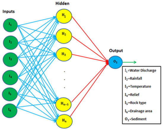
Figure 2.
Architecture of MLP-based ANN.
The weight (W) of the LM in ANN depends on the Jacobian matrix (), identity matrix (), iteration number (), error matrix (), and combinational coefficient of LM () during the learning processes. Figure 3 shows the overall layout of the proposed ANN method.
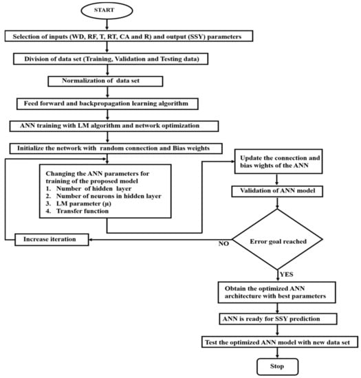
Figure 3.
The flowchart of the proposed ANN model with heuristic parameters selection processes for SSY prediction.
Unlike other temporal variables, spatial input variables, such as RT, R, and CA, are fixed for each gauging station and do not change (WD, RF, T, and SSY) in ANN model development. The RT value was mapped between 0 and 1. The RT value is 0 if any gauge station has a very hard rock with the lowest weatherability. If the RT is soft, such as clay, limestone, or other materials that dissolve and weather quickly, the RT value was set to 1. Similarly, the values of R and CA are mapped between 0 and 1. The highest R-value in a gauge station inside the river basin is 1, and the lowest R-value in a gauge station is 0, with the values in between linearly interpolated between 0 and 1. To obtain values between 0 and 1, the catchment region was also coded similarly to R. The ANN prediction model is developed using these data. The performance of the ANN model is evaluated with other existing regression-based methods, such as SRC and MLR.
The relationship between SSY and WD is given by the SRC method as a power function that is nonlinear [5,24]:
where and indicate the coefficients of the SRC regression method. The generalized least square method was used to perform linear regression between the (WD) and log (SSY) data to determine the values of and . The direct relationship between SSY and WD is examined using the SRC method. In place of the original data, normalized data is used for the SRC method. The performance evaluation of the SRC method is compared with ANN and MLR models on the same test data set.
The MLR method is the widely known regression method to predict SSY through a linear combination of the input and output variables. The MLR model involves the fitting of a linear equation between two or more dependent variables and independent variables. SSY prediction has been conducted in past research using a conventional MLR approach [20,21]. The MLR model is developed using hydro-geo-climatically data (WD, RF, T, CA, RT, R, and SSY) from 11 gauging stations. The MLR method is considered for the prediction of the SSY linearly using the input variables. The MLR formula can be expressed as
where is the regression intercept; , , , and are the coefficients of the input variables WD, RF, T, CA, RT, and R, respectively. The MLR represents the dependent predicted output, through the independent input variables at time (). The least square regression method was applied to calculate the values of , , , , , , and coefficients of the MLR using input and observed output data.
4. Results and Discussion
Analysis of variance (ANOVA) was used to select the inputs. The ANOVA test is used to determine whether all input parameters (WD, RF, T, and CA) are statistically different or not. Figure 4 shows the box plots results of the ANOVA test. It was noticed that all of the input parameters have different distributions because of differences in the central lines of the individual boxes which represent the mean value of individual boxes of each input. As a result, it was decided to consider all of these input parameters when predicting SSY in the MRB. In past research, some researchers have used ANOVA analysis for input parameter selections in modeling which are well described in various literature [25,55,56,57]. Bastia and Equeenuddin [37] demonstrated that water discharge, rainfall, catchment area, etc. affect the sediment yield in the Mahanadi River basin. Temperature also plays an important role in the erosion rate or sediment yield, which are the dominant driving forces of sediment transportation and sediment generation [20,58]. Temperature influences sediment yield in many indirect ways. Temperature changes may affect sediment discharge by altering runoff and changing the rate of erosion due to their effects on vegetation, evapotranspiration, and weathering [20,59]. However, several studies show that temperature is exponentially related to sediment load and erosion rate [60,61]. Therefore, in this study, the temperature was included as one of the inputs in the sediment yield model. In the ANOVA boxplot, the red color plus (+) of the water discharge and rainfall represents outliers, which are data values that are far away from other data values which can strongly affect the results. Often outliers are easiest to identify on an ANOVA boxplot. Water discharge and rainfall data are skewed. The majority of the data in the ANOVA plot are located on the high or low side of the graph. The data set may be left-skewed or right-skewed. Skewed data indicates that the data might not be normally distributed. It has been found that a high value of the skewness coefficient has a considerable negative influence on the performance of the artificial neural network (ANN) [62]. Analysis of Variance (ANOVA) test results of the hydro climatical data set are shown in Table 3.
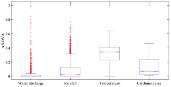
Figure 4.
ANOVA test result of the input data.
Table 3.
Analysis of Variance (ANOVA) test results of the hydro climatical data set.
The ANOVA results show the between-groups variation (Columns) and within-groups variation (Error). In the ANOVA test, the values of sum of squared error (SS), degree of freedom (Df), mean squared error (MS), F-statistics, and error are given in Table 3. MS is the ratio between the SS and Df for each source of variation. The total degrees of freedom are the total number of observations minus one. The between-groups degree of freedom is the number of groups minus one. The within-groups degree of freedom is the total degrees of freedom minus the between-groups degree of freedom. The F-statistic is the ratio of the mean squared errors. The p-value is the probability that the test statistic can take a value greater than the value of the computed test statistic which is equal to 0.001. The small p-value of 0.001 indicates that differences between column means are significant.
Yadav et al. [24] and Yadav et al. [25] demonstrated that suspended sediment yield is very closely related to water discharge in comparison to rainfall and temperature. Temperature has a stronger relationship with rainfall, which has a stronger relationship with suspended sediment yield. Temperature is related to suspended sediment yield in a secondary way. Thus, temperature influences sediment yield in a variety of indirect ways. Temperature has the lowest impact on sediment yield as compared to rainfall and water discharge. It was found that water discharge, rainfall, catchment area, and temperature etc. are the most dominant controlling factors of the suspended sediment yield in the Mahanadi River [24,25,26,27]. The variation in WD, T, RF, and SSY at different locations with different periods (months) is shown in Figure 5. There is exhibit significant fluctuation in WD and SSY among all temporal variables in the MRB across time without any cyclic pattern.
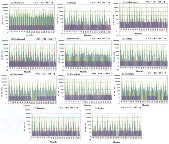
Figure 5.
Monthly variations in WD, RF, T, and SSY at different locations (a) Tikarapara (b) Simga (c) Andhiyarakhore (d) Sundargarh (e) Bamnidih (f) Jondhra (g) Kantamal (h) Kurubhata (i) Basantpur (j) Baronda (k) Rajim.
The inputs, outputs, and neurons with a hidden layer are used for developing the ANN model using temporal and spatial data for SSY prediction. The combination coefficient of LM (µ) value was kept flexible throughout this ANN modeling process which ranged from 0.001 to 10 × 109, and the value was incremented and reduced by a factor of ten and 0.1, respectively. The model began with a random connection and bias weights values that were initialized and then updated every epoch to optimize performance. In this study, the maximum number of hidden neurons was restricted to 32, in view of computational time and model complexity [25,49,50]. The lower the complexity of the model, the easier it is to understand the interpretability of the artificial intelligence model [63]. Figure 6 shows the RMSE variation values with neurons an µ of the ANN using grid search techniques. This figure shows that when the optimum neurons in the hidden layer and µ are 31 and 0.06, respectively, then the ANN model produced the lowest RMSE value (0.00460) in the training phase. As a result, it was considered the best ANN model. To examine the effectiveness of the models, the error variance (VAR), RMSE, mean absolute error (MAE), coefficient of efficiency (CE), mean square error (MSE), and correlation coefficient () are often utilized as statistical performance measures.
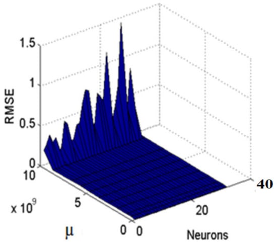
Figure 6.
Effect of Neurons and µ on RMSE during the training of the ANN model.
Table 4 indicates the error statistics of the ANN model’s training, validation, and testing data sets. If the model is ideal, RMSE, MSE, VAR, and MAE should be around zero, while CE and r should be near one. For all three data sets, the RMSE is extremely low (0.00457–0.01096) and r is significantly higher (0.7414–0.9757). According to the RMSE and r value, it can be inferred that this ANN model predicts SSY with higher accuracy. The error statistics data revealed that RMSE and MAE exhibit comparable tendencies. According to the results, these are in direct proportion to one another. The SSY significantly strongly correlated at all gauging stations except Andhiyarakhore, Sundargarh, and Bamnidih. Tikarapara gauging station had the highest r (0.9675) value among all stations. The Pearson correlation coefficient (r) should be justified as being strong if the r value is greater than 0.7, moderate if it is between 0.5 and 0.7, and poor if it is less than 0.5 [9]. According to Legates and McCame [64], the Pearson correlation coefficient (r) is not necessarily appropriate for evaluating hydrological models. As a “goodness-of-fit” measure, the CE is a good substitute for r.
Table 4.
Error statistics during the testing, training, and validation phases of the ANN model of 11 gauge stations of the MRB.
The value of the coefficient of efficiency (CE) fluctuated between −29.4624 and 0.9518. At Andhiyarakhore, Simga, and Bamnidih, the CE value was negative, indicating that the model’s performance was worse than the observed mean value. Kurubhata (0.160) had small positive values of CE, which were near zero. The CE value of 0 shows that the model is unable to predict the actual values, as measured by the observed mean [65]. The CE at Tikarapara was 0.901 which is almost 1 and the greatest among all the stations that demonstrate the proposed model provided superior performance at Tikarapara.
The ANN model appears to have reasonable accuracy in estimating SSY for all other stations, with CE ranging from 0.4116 to 0.7849. Negative CE values were reported at Bamnidih (−29.46), Simga (−0.196), and Andhiyarakhore (−14.88) which indicates poor performance. Aside from quantitative assessment using statistical measures, the efficiency of the ANN in predicting SSY at 11 gauging stations was evaluated using diagrammatical indicators. Figure 6 and Figure 7 depict the hydrograph and scatter graph between estimated ANN and observed SSY with time (months). Except for Simga, Bamnidih, Kurubhata, and Andhiyarakhore, the hydrographs show that the predicted SSY follow the variation of the observed data. Similarly, in the scatter plot of the ANN, except for the above-mentioned gauging stations, the points of data were scattered around the 45-degree line (1:1 line). This line is a bisector line that has the same predicted and observed values. If the scatter points are close together along this line, the predicted and observed values are approximately the same. If all scatter values fall along this line, this is a perfect model.
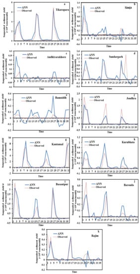
Figure 7.
Hydrograph between predicted SSY and actual SSY of testing data of the ANN prediction model.
The modeled SSY in both Andhiyarakhore and Bamnidih stations showed wide variations in all peaks and corresponded to a low value of observed SSY when compared to other gauging stations. The ANN estimated SSY values were nearest to the actual data values at Tikarapara among all stations, as seen in both plots. Furthermore, the model provides accurate estimates in Jondhra, Sundargarh, Kantamal, Baronda and Basantpur. The scatter plot between both the estimated and actual values (Figure 8a) of the ANN model also shows that the majority of the scatter points are near the bisector line. The ANN model did not perform well in predicting SSY at Bamnidih, Andhiyarakhore, Kurubhata, and Rajim stations.
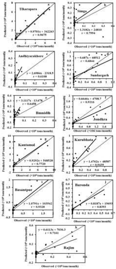
Figure 8.
Scatter plots between predicted SSY and actual SSY of testing data of the ANN prediction model.
In comparison to other gauge stations, a large number of negative estimated values were produced by the model at Bamnidih and Andhiyarakhore; although, SSY cannot be negative in actuality. SSY at these sites was found to be highly non-linear. At Bamnidih, a considerable discrepancy between the bisector line and the linear regression line can also be seen from the scatter plot. The hydrograph also shows that at these sites, the observed and model SSY did not match up. It could be because of the big Minimata Bango dam before this station. The hydrologic graph and scatter plots reveal that the proposed model did not produce satisfactory results in Andhiyarakhore. It could be because of the low CA. The poor performance of the proposed ANN model for predicting suspended sediment at Andhiyarakhore, Bamnidih, Rajim, and Kurubhata stations can be attributed to the highly complicated interaction of several suspended sediment yield controlling factors. Kurubhata and Andhiyarakhore are two small tributaries with relatively small catchment areas; however, these carry relatively high suspended sediment yield. It is because of the inability of relatively small basins to store sediments and allow all eroded material to be removed [66]. The presence of a large Minimata Bango dam at Bamnidih is the primary cause of modeled output deviation. Simga has a relatively large catchment area, but its topography is very flat and dominated by limestone. As a result, the sediment yield and water discharge are low in comparison to other tributaries–Seonath and Tel that have a small catchment area. The hydrograph and scatter plots show that the ANN model provided the highest accuracy at Tikarapara station and the lowest accuracy at Andhiyarakhore and Bamnidih gauging stations (Figure 7 and Figure 8). The ANN model also provided satisfactory performances and the best result at Tikarapara gauging station among all gauging stations which may be due to the highest WD, CA, SSY, and RF among all gauging stations at this gauging station.
After the development of a reliable ANN model, the model’s performance was evaluated using the same testing data that was not utilized during the training phase. The ANN models at Tikarapara (ANN-1) were developed using just the data from this station and the same ANN model methods with temporal data (WD, RF, and T) as inputs. The comparison has been based on the test data’s estimated values and the same actual testing data for both models. Table 5 displays the error statistics obtained in the testing phase, such as MSE, MAE, RMSE, VAR, and values of all models.
Table 5.
Performance comparisons in testing data error statistics of the ANN model and ANN-1 model of Tikarapara Station of the MRB.
According to this table, the ANN model has a lower RMSE than the ANN-1, SRC, and MLR models. As a result, the ANN model outperformed the ANN-1 model. Based on the result, it was realized that the ANN model has greater generalization capability than that of the individual models of different gauging stations. It provided a superior result than the ANN-1 of Tikarapara station because the ANN model used combined inputs (WD, RF, T, RT, R, and CA) data from 11 gauging stations. The ANN model of Tikarapara (ANN-1) was also developed by considering these inputs but it is less capable than the ANN model of all stations because it was developed by considering a single station so it has a decreased generalization capability. It is observed from the hydrograph and scatter plots of the ANN model that the predicted and observed sediment was closer than the ANN-1 model (Figure 7, Figure 8 and Figure 9).
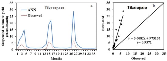
Figure 9.
(a) Hydrograph between the predicted and actual SSY at Tikarapara using the ANN-1 model; (b) Scatter plot between the predicted SSY and actual at Tikarapara using the ANN model.
The hydrographs in Figure 7 and Figure 9a indicate that the proposed and observed SSY of the ANN model are closer than in the ANN-1 model. The scatter plots of Figure 7b and Figure 9b also show that the ANN-1 model has a larger deviation between the bisector and regression line than the ANN model. The ANN model’s superiority may be due to the development of this model using the combined data of 11 gauging stations as training by taking inputs, such as (WD, RF, T, RT, R, and CA) instead of considering Tikarapara data only and the inclusion of spatial data (RT, R, and CA) also. This ANN model has a greater generalization capability compared to the ANN-1 model.
The MLR, ANN, and SRC model performance assessments were conducted for all 11 stations during the test period (Table 5). In comparison to MLR (RMSE-0.00896; r-0.843) and SRC (RMSE-0.01010; r-0.792), ANN models had the lowest RMSE (0.00892) and greatest r (0.867). As a result, based on these error statistics, the ANN model performed better than MLR and SRC. The ANN method’s efficiency in estimating SSY at 11 gauging stations also can be evaluated using graphical indications.
Particularly at high sediment values, it can be seen in the hydrographs that the estimated SSY by the ANN model is closer to the actual observations than the SRC and MLR (Figure 7, Figure 10, Figure 11 and Figure 12). The SRC model produced poor performances, which significantly underestimated the peaks and failed to catch the abnormally high SSY. Thus, it provided the worst performance among all models. The actual and estimated SSY values in the ANN model are closer than the SRC model (Figure 7 and Figure 12). In the scatter plots (Figure 8, Figure 11 and Figure 13), it is seen that the MLR model estimated more negative SSY at a low value as compare to other ANN and SRC models. It indicates the complex non-linear behavior of sedimentation at low sediment yields which are not captured by the model. However, the ANN model provided a high number of positive sediment values as compared to ANN-1, MLR, and SRC even when the SSY was low (Figure 7, Figure 8, Figure 9, Figure 10, Figure 11, Figure 12 and Figure 13). These results reveal that the ANN approach provides better performance and generalization capability than other comparative methods. In the hydrographs, it is also noticed that the estimated SSY by the ANN model is nearest to the actual SSY as compared to ANN-1, MLR, and SRC at Tikarapara (Figure 7a, Figure 8a, Figure 9a, Figure 10a, Figure 11a, Figure 12a and Figure 13a). As seen in the scatter plots of all models, the ANN-based linear regression line is much closer to the 45-degree line than the SRC, ANN-1, and MLR-based models. Thus, particularly in comparison to other ANN-1, MLR, and SRC models, the ANN model was found to be the most capable (Figure 7b, Figure 8b, Figure 9b, Figure 10b, Figure 11b, Figure 12b and Figure 13b).
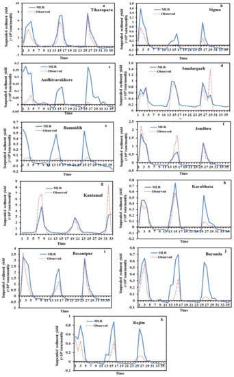
Figure 10.
Hydrograph between the predicted and actual SSY of testing data of the MLR model.
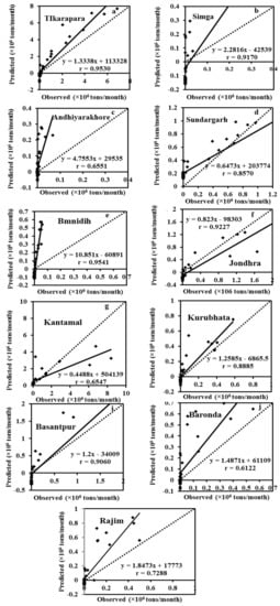
Figure 11.
Scatter plots between predicted and actual SSY of testing data of the MLR model.
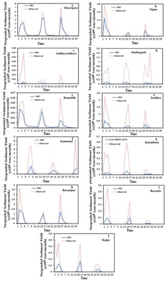
Figure 12.
Hydrograph between predicted and actual SSY of testing data of the SRC model.
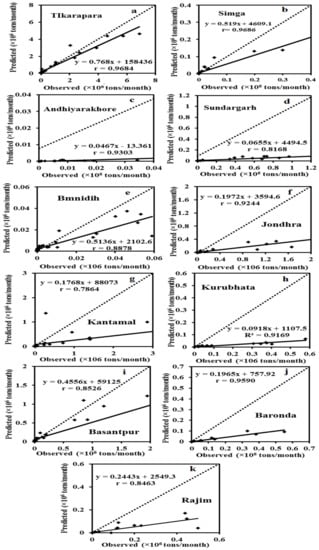
Figure 13.
Scatter between the predicted and actual SSY of testing data of the SRC model.
5. Conclusions and Future Scope
It may be concluded that the SSY patterns in the MRB are largely controlled by RF, WD, T, RT, R, and CA. It was found that the MRB’s WD and SSY show large oscillations, whereas T and RF show little variance among gauge stations in the basin. Furthermore, Tikarapara has the highest WD, RF, CA, and SSY, whereas Andhiyarakhore has the lowest SSY, WD, RF, and CA. In comparison to other hydro-climatic variables (WD, RF, and T), SSY has more non-linear complex processes. The far downstream Tikarapara station of the MRB had the highest WD, RF, CA, and SSY, whereas the upstream Andhiyarakhore station had the lowest WD and SSY. The models cannot estimate SSY with high accuracy at gauge stations that have extremely very small CAs but perform well at moderate to large CA sites. At Tikarapara, the gauge station far downstream with the highest CA, the models produced the best results. If there are no SSY measurements available in any river, the modeling approach can be used to estimate SSY at gauged or ungagged places. Hydro-climatic variables (WD, T, RF, RT, R, and CA) were found to be the most important governing parameters of SSY in the MRB. Thirty-one hidden neurons were found to be the most suitable for the ANN model for obtaining satisfactory results. A greater proportion of negative values were produced by the proposed ANN model at Bamnidih and Andhiyarakhore among all gauging stations, which do not exist in reality. The modeled SSY indicates significant fluctuation in all peaks and during low SSY at both Bamnidih and Andhiyarakhore stations. High nonlinearity was found in Bamnidih and Andhiyarakhore stations. Among all gauging stations, the developed model was particularly effective at estimating SSY at Tikarapara station. It has been concluded that the ANN model, which is based on data from 11 stations, is the most suitable substitute and has a greater generalization capacity than the ANN-1 model, which is based on data from only the WD, RF, and T of Tikarapara station. It was also noticed that the ANN performed better than ANN-1, MLR, and SRC models. The study used rainfall data instead of rainfall intensity. It is also obvious that rainfall intensity would be much more significant than quantity because the detachment of the soil is more influenced by intensity than quantity of rain. The rainfall intensity factor was not incorporated into this research for the improvement of modeling performance due to its unavailability at gauging stations in the MRB but will be addressed in future research. Anthropogenic activities are not included in this study, but these factors are critical for SSY prediction. As a result, these variables will be considered in future studies.
Author Contributions
Conceptualization, D.J., P.C. and A.Y.; methodology, A.Y., P.C. and A.S.; software, A.Y., P.C. and D.H.E.; validation, A.Y., P.C. and C.M.P.-O.; analysis, D.J., P.C. and A.S.; investigation, D.A.; resources, A.S. and D.H.E.; writing—original draft preparation, D.J. and P.C.; writing—review and editing, D.J., P.C., A.S. and A.Y.; supervision, A.S. and D.A.; project administration, C.M.P.-O. All authors have read and agreed to the published version of the manuscript.
Funding
The research was funded by Princess Nourah bint Abdulrahman University Researchers Supporting Project number (PNURSP2022R238), Princess Nourah bint Abdulrahman University, Riyadh, Saudi Arabia.
Data Availability Statement
The authors would like to express their thanks to the Central Water Commission, Odisha for provided the data. The author honorable thanks to the National Institute of Technology, Rourkela, India, for offering the necessary facilities for this research.
Acknowledgments
The authors acknowledge Princess Nourah bint Abdulrahman University Researchers Supporting Project number (PNURSP2022R238), Princess Nourah bint Abdulrahman University, Riyadh, Saudi Arabia.
Conflicts of Interest
The authors declare that they have no conflict of interest.
References
- Hasnain, S.I.; Thayyen, R.J. Discharge and suspended-sediment concentration of meltwaters, draining from the Dokriani glacier, Garhwal Himalaya, India. J. Hydrol. 1999, 218, 191–198. [Google Scholar] [CrossRef]
- Kisi, O.; Yaseen, Z.M. The potential of hybrid evolutionary fuzzy intelligence model for suspended sediment concentration prediction. Catena 2019, 174, 11–23. [Google Scholar] [CrossRef]
- Chang, H.H. Case Study of Fluvial Modeling of River Responses to Dam Removal. J. Hydraul. Eng. 2008, 134, 295–302. [Google Scholar] [CrossRef]
- Kisi, O. Constructing neural network sediment estimation models using a data-driven algorithm. Math. Comput. Simul. 2008, 79, 94–103. [Google Scholar] [CrossRef]
- Yadav, A.; Prasad, B.B.V.S.V.; Mojjada, R.K.; Kothamasu, K.K.; Joshi, D. Application of Artificial Neural Network and Genetic Algorithm Based Artificial Neural Network Models for River Flow Prediction. Rev. Intell. Artif. 2020, 34, 745–751. [Google Scholar] [CrossRef]
- Safari, M.J.S.; Mohammadi, B.; Kargar, K. Invasive weed optimization-based adaptive neuro-fuzzy inference system hybrid model for sediment transport with a bed deposit. J. Clean. Prod. 2020, 276, 124267. [Google Scholar] [CrossRef]
- ASCE. Task Committee on Application of Artificial neural networks in Hydrology, Artificial neural networks in hydrology. I: Preliminary concepts. J. Hydrol. Eng. 2020, 5, 115–123. [Google Scholar]
- Maier, H.R.; Dandy, G.C. Neural network for the prediction and forecasting of water resources variables: A review of modeling issues and applications. Environ. Model. Softw. 2000, 15, 101–124. [Google Scholar] [CrossRef]
- Sahoo, S.; Jha, M.K. Groundwater-level prediction using multiple linear regression and artificial neural network techniques: A comparative assessment. Hydrogeol. J. 2013, 21, 1865–1887. [Google Scholar] [CrossRef]
- Shamseldin, A.Y. Application of a neural network technique to RF-runoff modeling. J. Hydrol. 1997, 199, 272–294. [Google Scholar] [CrossRef]
- Zealand, C.; Burn, D.H.; Simonovic, S.P. Short term streamflow forecasting using artificial neural networks. J. Hydrol. 1999, 214, 32–48. [Google Scholar] [CrossRef]
- Imrie, C.E.; Durucan, S.; Korre, A. River flow prediction using artificial neural networks: Generalization beyond the calibration range. J. Hydrol. 2000, 233, 138–153. [Google Scholar] [CrossRef]
- Melesse, A.M.; Wang, X. Multi-temporal scale hydrograph prediction using artificial neural networks. J. Am. Water Resour. Assoc. 2006, 42, 1647–1657. [Google Scholar] [CrossRef]
- Ahmad, S.; Simonovic, S.P. An artificial neural network model for generating hydrograph from hydro-meteorological parameters. J. Hydrol. 2005, 315, 236–251. [Google Scholar] [CrossRef]
- Zhang, Q.; Stanley, S.J. Forecasting raw-water quality parameters for the North Saskatchewan River by neural network modeling. Water Res. 1997, 31, 2340–2350. [Google Scholar] [CrossRef]
- Melesse, A.; Jayachandran, K.; Zhang, K. Modeling coastal eutrophication at Florida Bay using neural networks. J. Coast. Res. 2008, 24, 190–196. [Google Scholar] [CrossRef]
- Solomatine, D.P.; Torres, L.A. Neural network approximation of a hydrodynamic model in optimizing reservoir operation. In Proceedings of the 2nd International Conference on Hydroinformatics, Zurich, Switzerland, 9–13 September 1996; pp. 201–206. [Google Scholar]
- Wen, C.G.; Lee, C.S. A neural network approach to multi-objective optimization for water quality management in a river basin. Water Resour. Res. 1998, 34, 427–436. [Google Scholar] [CrossRef]
- Brion, G.M.; Lingireddy, S. A neural network approach to identifying non-point sources of microbial contamination. Water Res. 1999, 33, 3099–3106. [Google Scholar] [CrossRef]
- Zhu, Y.M.; Lu, X.X.; Zhou, Y. Suspended sediment flux modeling with artificial neural network: An example of the Longchuanjiang River in the Upper Yangtze Catchment, China. Geomorphology 2007, 84, 111–125. [Google Scholar] [CrossRef]
- Rajaee, T.; Mirbagheri, S.A.; Zounemat-Kermani, M.; Nourani, V. Daily suspended sediment concentration simulation using artificial neural network and neuro-fuzzy models. Sci. Total Environ. 2009, 407, 4916–4927. [Google Scholar] [CrossRef]
- Melesse, A.M.; Ahmad, S.; McClain, M.E.; Wang, X.; Lim, Y.H. Suspended Sediment Load Prediction of River Systems: An artificial neural network approach. Agric. Water Manag. 2011, 98, 855–866. [Google Scholar] [CrossRef]
- Sharma, N.; Zakaullah, M.; Tiwari, H.; Kumar, D. Runoff and sediment yield modeling using artificial neural network and support vector machines: A case study from Nepal watershed, Model. Earth Syst. Environ. 2015, 1, 23. [Google Scholar] [CrossRef]
- Yadav, A.; Chatterjee, S.; Equeenuddin, S.M. Suspended sediment yield Estimation using Genetic Algorithm-based Artificial Intelligence Models in Mahanadi River basin. Hydrol. Sci. J. 2018, 63, 1162–1182. [Google Scholar] [CrossRef]
- Yadav, A.; Chatterjee, S.; Equeenuddin, S.M. Prediction of Suspended Sediment Yield by ANN and Traditional Mathematical Model in MRB, India. Sustain. Water Resour. Manag. 2017, 4, 745–759. [Google Scholar] [CrossRef]
- Yadav, A.; Satyannarayana, P. Multi-objective genetic algorithm optimization of artificial neural network for estimating suspended sediment yield in Mahanadi River basin, India. Int. J. River Basin Manag. 2020, 18, 207–215. [Google Scholar] [CrossRef]
- Yadav, A. Estimation and Forecasting of Suspended Sediment Yield in Mahanadi River Basin: Application of Artificial Intelligence Algorithms; NIT Rourkela: Orissa, India, 2019. [Google Scholar]
- Yadav, A.; Joshi, D.; Kumar, V.; Mohapatra, H.; Iwendi, C.; Gadekallu, T.R. Capability and Robustness of Novel Hybridized Artificial Intelligence Technique for Sediment Yield Modeling in Godavari River, India. Water 2022, 14, 1917. [Google Scholar] [CrossRef]
- Yadav, A.; Chatterjee, S.; Equeenuddin, S.M. Suspended sediment yield modeling in Mahanadi River basin, India by multi-objective optimization hybridizing artificial intelligence algorithms. Int. J. Sediment Res. 2021, 36, 76–91. [Google Scholar] [CrossRef]
- Pramanik, N.; Panda, R.K. Application of neural network and adaptive neuro-fuzzy inference systems for river flow prediction. Hydrol. Sci. J. 2009, 54, 247–260. [Google Scholar] [CrossRef]
- Kar, A.K.; Lohani, A.K.; Goel, N.K.; Roy, G.P. Development of Flood Forecasting System Using Statistical and artificial neural network Techniques in the Downstream Catchment of Mahanadi Basin, India. Water Resour. Prot. 2010, 2, 880–887. [Google Scholar]
- Meher, J. RF and Runoff Estimation Using Hydrological Models and ANN Techniques. Ph.D. Thesis, National Institute of Technology, Rourkela, India, 2014. [Google Scholar]
- Samantaray, S.; Ghose, D.K. Evaluation of suspended sediment concentration using descent neural networks. Procedia Comput. Sci. 2018, 132, 1824–1831. [Google Scholar] [CrossRef]
- Kant, A.; Suman, P.K.; Giri, B.K.; Tiwari, M.K.; Chatterjee, C.; Nayak, P.C.; Kumar, S. Comparison of multi-objective evolutionary neural network, adaptive neuro-inference system and bootstrap-based neural network for flood forecasting. Neural. Comput. Appl. 2013, 23, 231–246. [Google Scholar] [CrossRef]
- Asokan, S.; Dutta, D. Analysis of water resources in the Mahanadi River basin, India under projected climate conditions. Hydrol. Process 2008, 22, 3589–3603. [Google Scholar] [CrossRef]
- India-WRIS, Water Resources Information System of India. 2015. Available online: http://india-wris.nrsc.gov.in/wrpinfo/index.php?title=Mahanadi (accessed on 8 August 2016).
- Bastia, F.; Equeenuddin, S.M. Spatio-temporal variation of water flow and sediment discharge in the MRB, India. Glob. Planet. Chang. 2016, 144, 51–66. [Google Scholar] [CrossRef]
- Chakrapani, G.J.; Subramanian, V. Heavy metals distribution and fractionation in sediments of the Mahanadi River basin, India. Environ. Geol. 1993, 22, 80–87. [Google Scholar] [CrossRef]
- Bhattacharya, B.; Lobbrecht, A.H.; Solomatine, D.P. Neural networks and reinforcement learning in control of water systems. J. Water Resour. 2003, 129, 458–465. [Google Scholar] [CrossRef]
- Kumar, V. Evaluation of computationally intelligent techniques for breast cancer diagnosis. Neural Comput. Applic. 2021, 33, 3195–3208. [Google Scholar] [CrossRef]
- Kumar, V.; Lalotra, G.S. Predictive Model Based on Supervised Machine Learning for Heart Disease Diagnosis. In Proceedings of the IEEE International Conference on Technology, Research, and Innovation for Betterment of Society (TRIBES), Raipur, India, 17–19 December 2021; pp. 1–6. [Google Scholar] [CrossRef]
- Wang, Y.M.; Traore, S. Time-lagged recurrent network for forecasting episodic event suspended sediment load in typhoon prone area. Int. J. Phys. Sci. 2009, 4, 519–528. [Google Scholar]
- Haghizade, A.; Shui, L.T.; Goudarzi, E. Estimation of yield sediment using artificial neural network at basin scale. Aust. J. Basic Appl. Sci 2010, 4, 1668–1675. [Google Scholar]
- Singh, G.; Panda, R. Daily sediment yield modeling with artificial neural network using 10-fold cross validation method: A small agricultural watershed, Kapgari, India. Int. J. Earth Sci. Eng. 2011, 6, 443–450. [Google Scholar]
- Karayiannis, N.B.; Venetsanopoulos, A.N. ALADIN: Algorithms for learning and architecture determination. In Artificial Neural Networks; Springer: Berlin/Heidelberg, Germany, 1993; pp. 195–218. [Google Scholar]
- Cybenko, G. Approximation by superpositions of a sigmoidal function. Math. Control Signals Syst. 1989, 2, 303–314. [Google Scholar] [CrossRef]
- Hornik, K.; Stinchcombe, M.; White, H. Multilayer feed forward networks are universal approximators. Neural Netw. 1989, 2, 359–366. [Google Scholar] [CrossRef]
- Tang, Z.; Almeida, D.C.; Fishwick, P.A. Time series forecasting using neural networks vs. Box-Jenkins methodology. J. Simul. 1991, 57, 303–310. [Google Scholar]
- Chatterjee, S.; Bandopadhyay, S. Global neural network learning using genetic algorithm for ore grade prediction of iron ore deposit. Min. Resour. Eng. 2007, 12, 258–269. [Google Scholar]
- Chatterjee, S.; Bandopadhyay, S. Reliability estimation using a genetic algorithm-based artificial neural network: An application to a laud-haul-dump machine. Expert Syst. Appl. 2012, 39, 10943–10951. [Google Scholar] [CrossRef]
- Jin, L.; Whitehead, P.G.; Rodda, H.; Macadam, I.; Sarkar, S. Simulating climate change and socio-economic change impacts on flows and water quality in the Mahanadi River basin system, India. Sci. Total Environ. 2018, 637, 907–917. [Google Scholar] [CrossRef] [PubMed]
- Boukhrissa, Z.A.; Khanchoul, K.; le Bissonnais, Y.; Tourki, M. Compare the Ann and Sediment rating curve model for prediction of suspended sediment load in EI Kebir catchment, Algeria. J. Earth Syst. Sci. 2013, 122, 1303–1312. [Google Scholar] [CrossRef]
- Samarasinghe, S. Neural Networks for Applied Sciences and Engineering: From Fundamentals to Complex Pattern Recognition; CRC Press: Boca Raton, FL, USA, 2016; p. 555. [Google Scholar]
- Demuth, H.B.; Beale, M. Neural Network Toolbox for Use with MATLAB, Users Guide; The Mathworks Inc.: Natick, MA, USA, 1998. [Google Scholar]
- Bachiller, A.R.; Rodríguez, J.L.G.; Sánchez, J.C.R.; Gómez, D.L. Specific sediment yield model for reservoirs with medium-sized basins in Spain: An empirical and statistical approach. Sci. Total Environ. 2019, 681, 82–101. [Google Scholar] [CrossRef]
- Faraway, J. Practical Regression and ANOVA in R. 2002. Available online: http://cran.r-project.org/doc/contrib/Faraway-PRA.pdf (accessed on 18 October 2022).
- Patel, A.K.; Chatterjee, S. Computer vision-based limestone rock-type classification using probabilistic neural network. Geosci. Front. 2016, 7, 53–60. [Google Scholar] [CrossRef]
- Ghose, D.K.; Swain, D.P.C.; Panda, D.S.S. Sediment load analysis using ANN and GA. In Applied Mechanics and Materials; Trans Tech Publications Ltd.: Bach, Switzerland, 2012; Volume 110–116, pp. 2693–2698. [Google Scholar]
- Zhu, Y.M.; Lu, X.X.; Zhou, Y. Sediment flux sensitivity to climate change: A case study in the Longchuanjiang catchment of the upper Yangtze River, China. Glob. Planet. Change 2008, 60, 429–442. [Google Scholar] [CrossRef]
- Harrison, C.G.A. What factors control mechanical erosion rates? Int. J. Earth Sci. 2000, 88, 752–763. [Google Scholar] [CrossRef]
- Syvitski, J.P.M.; Peckham, S.D.; Hilberman, R.; Mulder, T. Predicting the Terrestrial Flux of Sediment to the Global Ocean: A Planetary Perspective. Sediment. Geol. 2003, 162, 5–24. [Google Scholar] [CrossRef]
- Altun, H.; Bilgil, A.; Fidan, B.C. Treatment of multidimensional data to enhance neural network estimators in regression problems. Expert Syst. Appl. 2007, 32, 599–605. [Google Scholar] [CrossRef]
- Jin, Y.; Sendhoff, B.; Korner, E. Evolutionary multi-objective optimization for simultaneous generation of signal-type and symbol-type representations. In Proceedings of the 3rd International Conference on Evolutionary Multi-Criterion Optimization, Guanajuato, Mexico, 9–11 March 2005; pp. 752–766. [Google Scholar]
- Legates, D.R.; McCabe, G.J. Evaluating the use of goodness-of-fit measures in hydrology and hydroclimatic model validation. Water Resour. Res. 1999, 35, 233–241. [Google Scholar] [CrossRef]
- Legates, D.R.; McCabe, G.J. A refined index of model performance: A rejoinder. Int. J. Climatol. 2013, 33, 1053–1056. [Google Scholar] [CrossRef]
- Chakrapani, G.J.; Subramanian, V. Factors controlling sediment discharge in the Mahanadi River Basin. India. J. Hydrol. 1990, 117, 169–185. [Google Scholar] [CrossRef]
Publisher’s Note: MDPI stays neutral with regard to jurisdictional claims in published maps and institutional affiliations. |
© 2022 by the authors. Licensee MDPI, Basel, Switzerland. This article is an open access article distributed under the terms and conditions of the Creative Commons Attribution (CC BY) license (https://creativecommons.org/licenses/by/4.0/).