Effects of Dynamic Land Use/Land Cover Change on Flow and Sediment Yield in a Monsoon-Dominated Tropical Watershed

Abstract

It is widely known that land use/land cover (LULC) changes significantly alter watershed hydrology and sediment yields. The impact, especially on erosion and sedimentation, is likely to be exacerbated in regions dominated by high rainfall patterns such as monsoons. This study analyzed the hydrological responses of LULC changes in terms of streamflow (SF) and sediment yield (SY) in a monsoon-dominated tropical watershed, the Periyar River Watershed (PRW) in Kerala, India. This watershed drains an area of 4793 km² characterized by an average monsoon rainfall of 2900 mm from June to November. The watershed hydrology and sediment dynamics were simulated using the Soil and Water Assessment Tool (SWAT) model for the impact assessment at the watershed outlet and the sub-watershed level. Historical LULC data were analyzed for 1988, 1992, 2002, and 2016 using the maximum likelihood method, and future LULC changes were projected for 2030, 2050, 2075, and 2100 using the Markov chain–cellular automata technique. Between 1988 and 2016, the urban area increased by 4.13 percent, while plantation and forest coverage decreased by 1.5 percent. At this rate, by 2100, the urban area is expected to grow by 16.45% while plantations and forest area will shrink by 13.7% compared to 1988. The effects of these changes on SF and SY were found to be minimal at the watershed outlet; however, at the spatial scale of sub-watersheds, the changes varied up to 70% for surface runoff and 200% for SY. These findings highlight the potential impacts of LULC changes in a monsoon-dominated watershed and may contribute to the development of successful LULC-based watershed management strategies for prevention of flooding and sediment loss.

1. Introduction

Changes in land use/land cover (LULC) cause a significant impact on flow processes and sedimentation [1,2,3,4,5,6,7,8]. Monitoring the effects of LULC changes on hydrology is crucial for managing watersheds and restoring their ecological balance. In recent years, hydrologists have been primarily concerned with quantifying the effect of changes in land use on the dynamics of streamflow in river basins. Moreover, as the scarcity of available water increases, the hydrologic community has focused considerable attention on the hydrologic effects of changes in LULC [9,10,11,12]. Changes in land use types, including farmlands, forests, and urban areas, have varying hydrological effects [13,14,15,16]. Compared to grassland, agricultural, and urban land uses, forest cover typically reduces streamflow [17]. In contrast, an increase in urbanization typically increases high streamflow and decreases low streamflow because infiltration decreases as the impervious surface increases [18]. Changes in particular vegetation types and species coverage have a substantial impact on the sediment load dynamics in river basins [19]. Evaluation of land use changes as a major sediment loading factor is essential for sediment routing management and the development of appropriate remedial measures [20]. Reductions in forest area and the expansion of agricultural land increase sediment yield [19,21].

The effect of LULC changes on hydrology and sediment yield varies across regions with different geological settings and climatic conditions. For example, in a humid tropical region, the change in streamflow is very high during wet seasons and relatively low during dry seasons [14,22]. In high-altitude regions such as the Himalayas, due to excessive deforestation, severe erosion and landslides are observed during intense thunderstorms, resulting in increased sediment load into water bodies. In urbanized areas, LULC changes trigger significant increases in runoff. In regions dominated by heavy rainfall in shorter periods of time (monsoon), rains often lead to flash floods, high runoff, and sedimentation losses due to the high intensity of the precipitation [15,18,23]. Due to this complex interconnection between LULC changes and watershed response, it is important to understand the dynamic change effect. Thus, strategically implementing LULC changes could play a vital role in successful watershed management, including preventing flooding and sediment loss.

Past studies have analyzed the role of LULC changes on flow, runoff, sediment yield, evapotranspiration, and other hydrological parameters [16,24,25,26,27,28,29]. These past studies used hydrological models such as the Soil and Water Assessment Tool (SWAT) for impact assessment analysis. [1,30,31]. In this study, the Periyar River Watershed (PRW), a monsoon-dominated watershed in the humid tropical Western Ghats of India, was selected to analyze the effect on streamflow and sediment yield due to historical and future projected changes in LULC. SWAT was used to develop a hydrologic model of the watershed. Historical LULC changes were analyzed using the maximum likelihood method, which forms the basis for future projections (near and far) of LULC using the Markov chain–cellular automata technique. The projected LULC changes were simulated using the calibrated model to analyze the changes in streamflow and sediment yield at the watershed outlet and the spatial changes in surface runoff generation and sediment yield at the sub-watershed level.

2. Materials and Methods

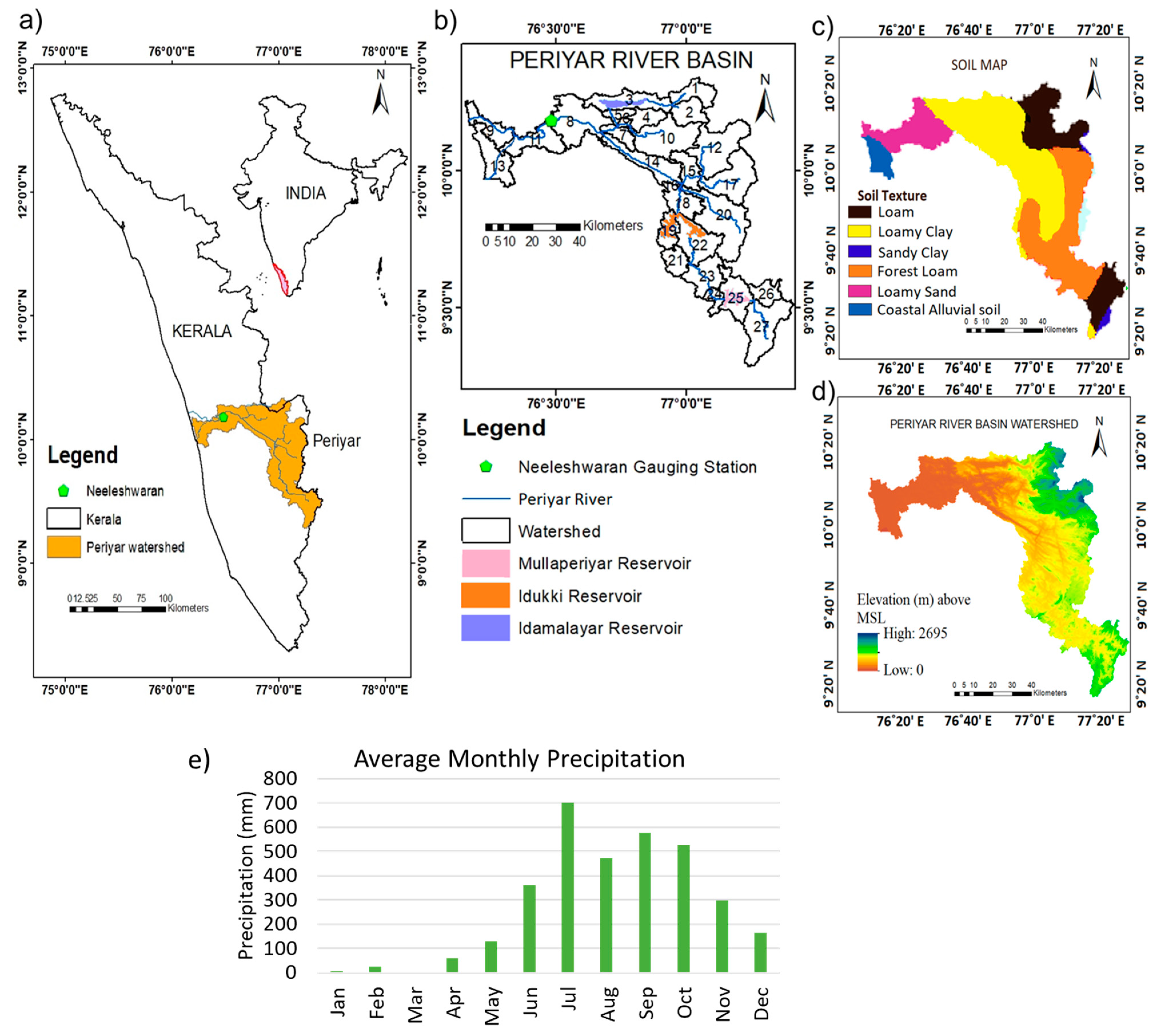
2.1. Study Area and Data Inputs

The Periyar River Watershed (PRW) is located in the central part of the state of Kerala, India (longitude 76°–77°30′ E and latitude 9°16′–10°20′ N, Figure 1). It is one of the largest river watersheds in Kerala state with a river length of 244 km and a total catchment area of 4792.83 km² (excluding the Chalakudy River catchment, which joins it near the Arabian Sea). According to the Köppen climate classification [32,33], the watershed belongs to the category of tropical monsoon climate with an average annual rainfall of 3200 mm [34]. The minimum and maximum temperature in PRW varies from 14 °C to 19 °C and 25 °C to 32 °C, respectively [35]. In PRW, approx. 90% of the annual precipitation is received during the two monsoon seasons, spanning six months: the southwest monsoon (June–mid September) and the northeast monsoon (October–November) (Figure 1e). Heavy precipitation concentration over a short time span leads to high flow and sedimentation losses in the watershed. To reduce such losses, several major and minor dams have been built across the river channel. The three major dams in PRW are Idamalayar Dam (capacity: 1089 million cubic meters (MCMs)), Idukki Dam(capacity: 5550 MCM), and Mullaperiyar Dam (capacity: 443.23 MCM) ( https://www.kseb.in/, (accessed on 15 February 2019) [36]). Sedimentation in these reservoirs is reducing their capacity and resulting in problems related to irrigation, hydropower generation, and flood control. There are certain flow restrictions from the Idukki and Mullaperiyar dams as water is transported outside the watershed due to water allocation policies increasing the complexity of the watershed. The major soil types are sandy/silty loams, alluvial, and forest loams (Figure 1c), as per National Bureau of Soil Survey and Land Use Planning (NBSS & LUP) soil classification (http://www.bhoomigeoportal-nbsslup.in (accessed on 1 February 2019)). The NBSS & LUP provides reliable soil data that have been used in various studies [27,37,38].

For the present study, the meteorological inputs required included precipitation, minimum and maximum temperature, wind speed, solar radiation, and relative humidity. These datasets were available in a gridded format at a daily scale from the India Meteorological Department (IMD) and Climate Forecast System Reanalysis (CFSR). Precipitation was available at 0.25° resolution [39], whereas temperature was available at 1° resolution [40]; these values were developed by the IMD from 395 quality control stations across the country. Wind and solar radiation were available at 0.5° resolution each from CFSR. All these datasets were re-gridded to 0.25° resolution using the linear interpolation technique. Other SWAT model inputs required were the digital elevation model (DEM), soil properties, land cover data, and slope data. The digital elevation model (DEM) at 30 m resolution was derived from CartoSAT satellite data, and the slope map was derived from the DEM (Figure 1d). The details of data availability, resolution, and sources are provided in

Table 1. Data Sources.

S. No.	Data Type	Resolution	Post Processing	Time Period	Source
1.	Topographic Input
	Digital Elevation Model	30 m × 30 m	-	2005	CartoDEM (bhvan.nrsc.gov.in)
	Soil Texture	30 arc second	-	2012	NBSS & LUP
2.	LULC	30 m × 30 m	-	1988, 1992, 2002, 2016	LandSAT (Earthexplorer.usgs)
3.	Gauge Discharge	Daily	-	1991–2004	Central Water Commission (CWC)
4.	Meteorological Data
	Precipitation	0.25° × 0.25°	0.25° × 0.25°	1991–2004	IMD
	Temperature	1.0° × 1.0°	0.25° × 0.25°	1991–2004	IMD
	Wind Speed	0.5° × 0.5°	0.25° × 0.25°	1991–2004	CFSR
	Solar radiation	0.5° × 0.5°	0.25° × 0.25°	1991–2004	CFSR

Note: NBSS & LUP: National Bureau of Soil Survey and Land Use Planning. IMD: India Meteorological Department. CFSR: Climate Forecast System Reanalysis (CFSR) data https://rda.ucar.edu/ (accessed on 1 February 2019).

.

2.2. Methods

2.2.1. LULC Classification and Markov Chain Projections

LISS-III LandSAT images were procured for the years 1988, 1992, 2002, and 2016 for the land use classification. These years were selected to show decadal change in watershed characteristics with varying LULC and based on the availability of data. Images were selected between the months of October and January) to obtain a clear representation of wetlands and vegetation as during this period the rainfall is reduced, and images are cloud-free. The maximum likelihood technique was used to classify the land use classes due to its advantages over other methods [41]. This technique has been readily applied in various studies to generate reliable LULC data [21,42,43,44]. In PRW, seven land use classes were identified, namely: water, urban, plantation (habitat plantation), mixed plantation–forest, thick forest, agriculture, and scrubland (wasteland). One hundred sample points for each land use class were selected for supervised classification and accuracy assessment. The overall accuracy and the kappa coefficient (κ) of the classified images varied between 84% and 93% and 0.81 and 0.87, respectively.

Future LULC maps were projected for the years 2030, 2050, 2075, and 2100. The Markov chain–cellular automata (MC-CA) technique was used to project the future LULC patterns due to its good ability to capture the trends [1,42,45,46,47]. The Land Change Modeler (LCM) developed by TerrSET software (https://clarklabs.org/terrset/land-change-modeler (accessed on 1 June 2019)) was used to apply the MC-CA algorithm on the LULC data for the years 1988 and 2002 to project LULC for the year 2016. The working principle of MC involves considering two images and identifying the transition trend from one class to another. A multi-layer perceptron artificial neural network (MLP-ANN) was fitted along with the driver variables (influencing elements) to develop a transition potential. These transition potential maps were used to project the future images. The projected LULC of 2016 was compared with the classified LULC of 2016 to validate the model and fix the driver variables. The same combination was used to project LULC for 2030, 2050, 2075, and 2100. The mathematical representation of the Markov model algorithm for the prediction of future land cover can be represented as follows [45]:

$$I_{t+1}=M_{mn}\ast I_t$$

(1)

where $I_t$ and $I_{t+1}$ are land cover maps at times t and t+1, respectively. $M_{mn}$ is the transition probability matrix from state m to n. $M_{mn}$ is represented as

$$M_{mn}=\left[\begin{array}{cccc}{M}_{11}& M_{12}& \dots & M_{1n}\\ M_{21}& M_1& \dots & M_{2n}\\ \dots & \dots & \dots & \dots \\ M_{m1}& M_{m2}& \dots & M_{mn}\end{array}\right]$$

(2)

Here, $M_{mn}$ should satisfy the following two conditions: $\sum _{m=1 n=1}^{m=i n=j}{M}_{mn}=1$ and $0<M_{mn}<1$.

2.2.2. Hydrological Model and Modeling Setup

The Soil and Water Assessment Tool (SWAT) is used for hydrological modeling with the ArcSWAT interface extension in the ArcMap GIS interface. SWAT is a physically based semi-distributed model developed by the U.S. Department of Agriculture (USDA) Agricultural Research Service [48]. The inputs used in SWAT include DEM, LULC, soil type, and weather parameters consisting of precipitation, temperature (minimum and maximum), relative humidity, wind speed, and solar radiation. SWAT is an efficient model for analyzing and predicting the behavior of hydrological changes in a watershed at the sub-watershed scale. The model can predict the impact of land management practices on sediment, water, and agriculture chemical yields in large watersheds [49]. It works on the water balance equation (Equation (3)) and covers all the components of the hydrological cycle of a region.

$$S{W}_t=S{W}_0+{\displaystyle \sum }_{i=1}^t\left(P_{day}-Q_{surf}-E_0-w_{seep}-Q_{gw}\right)$$

(3)

where $P_{day}$ is the amount of precipitation (mm), $E_0$ is evapotranspiration, $w_{seep}$ is the water entering the soil above the groundwater level (mm), $Q_{gw}$ is the return flow (m³/s) for t days, $Q_{surf}$ is the surface runoff (m³/s), $S{W}_0$ is the initial water content, and $S{W}_t$ is the final water content on the ith day. The Penman–Monteith equation, which uses the provided precipitation, temperature, wind, and relative humidity data as input, was used in this study to estimate potential evapotranspiration.

The model divides the watershed into sub-watersheds based on the information from the DEM. These sub-watersheds are further divided into homogeneous combinations of LULC, soil type, slope, etc. Based on these combinations, hydrologic response units (HRUs) are created [50]. Runoff is calculated using the SCS curve number method (USDA Soil Conservation Service, 1972) and channel routing via various storage methods. For sediment yield estimation, SWAT uses the modified universal soil loss equation (MUSLE) [48]. The modified universal soil loss equation is given by:

$$S_y=\alpha {\left(Q_{surf}\ast q_{peak}\ast A_{HRU}\right)}^{\beta }\ast K_{USLE}\ast C_{USLE}\ast P_{USLE}\ast L{S}_{USLE}\ast C$$

(4)

where $S_y$ is HRU-based sediment yield (tons/day); $q_{peak}$ is runoff peak discharge (m³/s); $Q_{surf}$ is daily surface runoff volume (mm water/ha); $A_{HRU}$ is HRU area (ha); $K_{USLE}$ is the USLE soil erodibility factor (metric ton m² ha/(m³ metric ton cm); $C_{USLE}$, $P_{USLE}$, and $L{S}_{USLE}$ are dimensionless factors accounting for HRU crop cover, soil protection, and topography; and $C$ is a unitless factor that accounts for coarse fragment cover [51].

The SWAT model was set up for the PRW based on topographic, hydrologic, and meteorological input with LULC data for the year 1992. The watershed after delineation was sub-divided into 27 sub-watersheds using the threshold drainage area method. The procedure used to obtain the optimum number of sub-basins was guided by the literature [52]. For monthly calibration and validation, the selected reference period was between 1991 and 2004 based on the availability of gauged discharge and sediment data at the watershed outlet (Neeleshwaram site) obtained from the Central Water Commission (CWC). The calibrated model was then analyzed for variation in streamflow and sediment yield with varying LULC between 1988 to 2100 (considering 1988 as the baseline). The model was executed with fixed meteorological, topographical, and hydrological parameters and changing LULC for 1988, 1992, 2002, 2016, 2030, 2050, 2075, and 2100.

3. Result and Analysis

3.1. LULC Change Analysis

Based on historical LULC and future projections, the LULC change analysis was carried out at the watershed and sub-watershed scales.

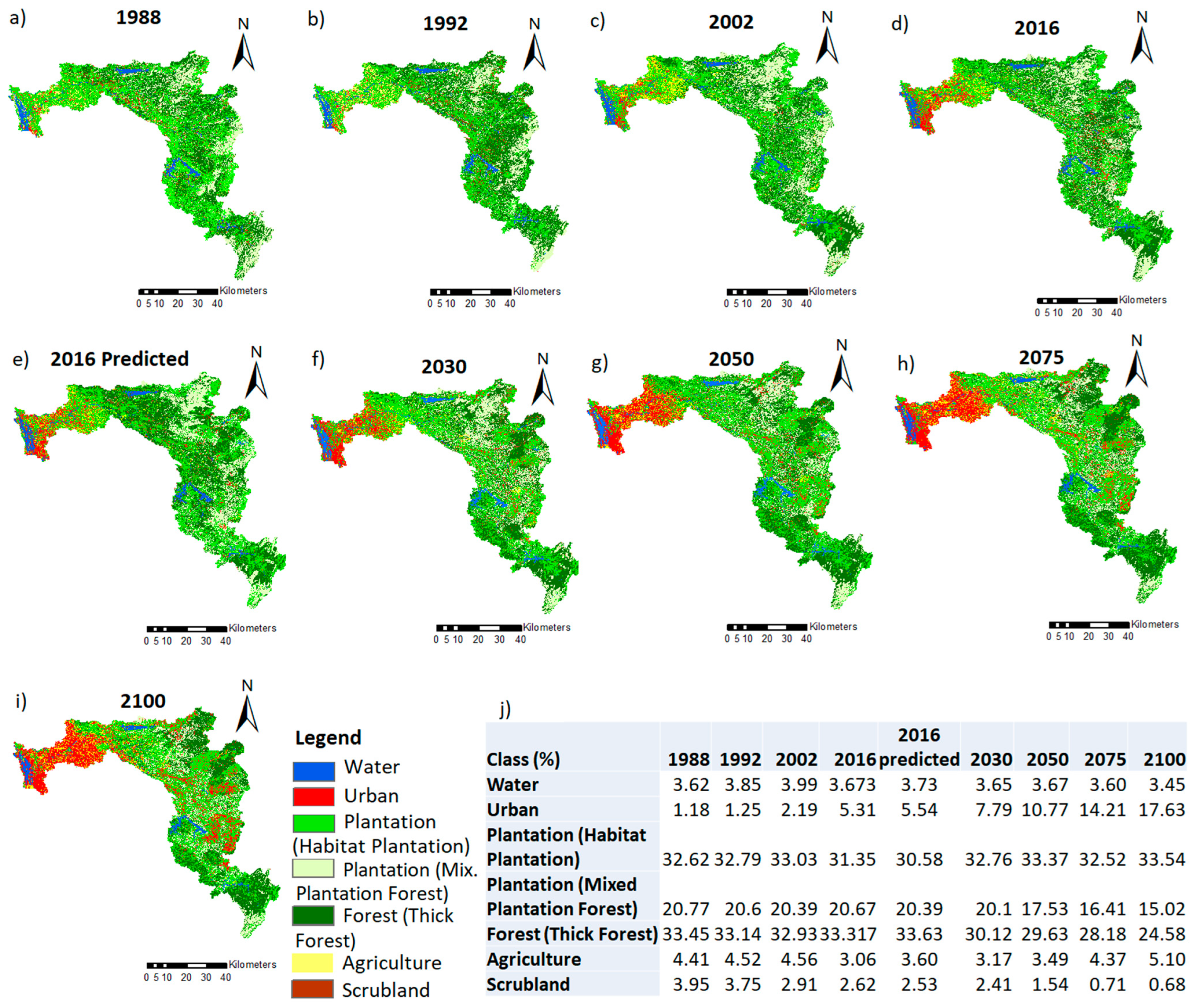
3.1.1. LULC Change at the Watershed Scale

In the year 1988, the PRW watershed was dominated by plantations (36.25%), followed by thick forests (31.82%) and mixed plantation–forest (18.77%) cover majorly distributed in the upstream and middle part. Water and urban areas accounted for 3.62%, and 1.18% of the watershed in 1988. The urban settlement was concentrated near the river channels and the downstream end. Agriculture area covered 4.41% and accumulated near the urban settlement. Small patches of scrubland (wasteland) were distributed in high-elevation areas and at the boundaries of water bodies (Figure 2a,j). The spatial distributions of the major LULC classes in 1988, 1992, 2002, and 2016 are shown in Figure 2a–d,j. Comparing the LULC data for the years 1988, 1992, 2002, and 2016, the most significant LULC changes occurred in the urban, plantation, and agricultural areas. From 1988 to 2016, the spatial coverage of urban areas increased to 4.36% of the watershed area (209 km²), which is an average increase of about 7.2 km²/year. As Figure 2a–d show, plantation and agricultural land were mainly converted to urban areas, whereas some spatial transition from plantation to agricultural land was also noticed. Around 60% of the area converted to urban spaces comprised plantations in 2016 (125.4 km²), and 20.2% comprised agricultural areas (42.22 km²). Furthermore, 85% of forest cover was retained, and the percentage of plantation area transitioning into forest area was 12.02%, while mixed plantation–forest comprised 8%. Agricultural land, scrubland, and mixed plantation–forest showed an overall decrease of 1.35% (64.7 km²), 1.33% (63.75 km²), and 0.10% (47.92 km²), respectively. The water area of the watershed was approximately the same with a nominal change of 0.05%.

For future projections, as discussed in Section 2.2.1, the LULC data for the years 1988, 1992, and 2002 were used to project the LULC in 2016 and compared with the classified LULC in 2016. With an accuracy above 86%, the driver variables were identified as the DEM, slope, distance from the road, built-up area, cropland, plantation, forest, and population density. Further, using this historical LULC transition, the future LULC was projected for the years 2030, 2050, 2075, and 2100, as shown in Figure 2f–i. For the future projections, the same trend was observed for urban area expansion, showing increases of 7.79%, 10.77%, 14.21%, and 17.63% for the years 2030, 2050, 2075, and 2100, respectively (Figure 2j). Agricultural land also followed the same increasing trend with an increase of 3.17% (151.93 km²) in 2030 to 5.10% (244.43 km²) in 2100. However, not much change was observed in overall plantation cover (varying between 32.5 and 33.5%) throughout the period of 2030 to 2100 (Figure 2j). Scrubland, water, and mixed plantation–forest showed reductions from 2.41 to 0.68%, 3.65 to 3.45%, and 20.1 to 15.02%, respectively, between 2030 and 2100.

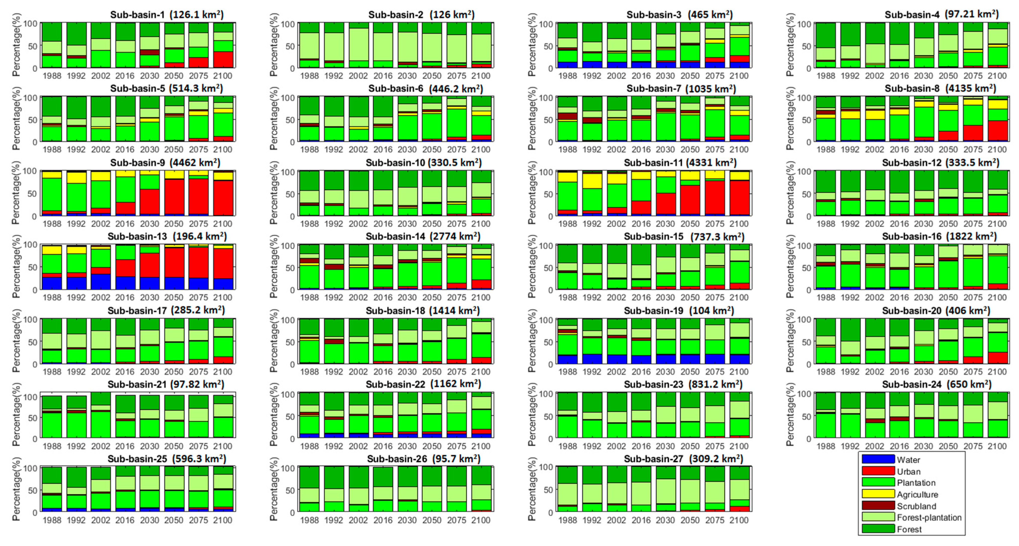
3.1.2. LULC Change at the Sub-Watershed Scale

Changes in LULC significantly alter the hydrological characteristics of the local region. Thus, it is important to study the changes in LULC at the sub-watershed scale in correlation with changes in variation in local hydrology. The PRW watershed is divided into 27 sub-watersheds based on topography. The variation in the LULC for each sub-watershed from 1988 to 2100 is represented in Figure 3. It can be noticed that in 1988, the urban concentration was limited to a few sub-watersheds, including sub-watersheds 8, 9, and 13.

Drastic urban growth was noticed in these sub-watersheds in 2016 with increases of 1.95% (2.57 km²), 9.66% (5.14 km²), and 27.65% (21.97 km²) in sub-watersheds 8, 9, and 13, respectively. Similarly, water bodies were limited to sub-watersheds 3, 9, 11, 13, 19, 22, and 25, and not much change was observed till 2016. Agricultural land was present in sub-watersheds 8, 9, 11, and 13. In 2016, the agricultural land comprised 13.13% (17.53 km²), 7.44% (3.96 km²), 18.6% (14.72 km²), and 2.31% (1.83 km²) of the area in sub-watersheds 8, 9, 11, and 13, respectively. The remaining sub-watersheds had major plantation and forest cover.

The future projections show that urban growth is expected to rise significantly and is not limited to just sub-watersheds 8, 9, and 13 but will also expand in sub-watersheds 1, 2, 3, 5, 6, 7, 11, 14, 15, 16, 17, 18, 20, 22, and 27 by the end of 2100. The agricultural area is expected to rise to 20.41% (26.91 km²), 9.02% (48.05 km²), 19.09% (15.11 km²), and 7.06% (5.61 km²) in sub-watersheds 8, 9, 11, and 13, respectively (Figure 3). Certain sub-watersheds, such as 23, 25, and 26, show minimal or no change in LULC area (Figure 3). These are the areas with no urban or agricultural area present and are mostly covered with forest and plantations.

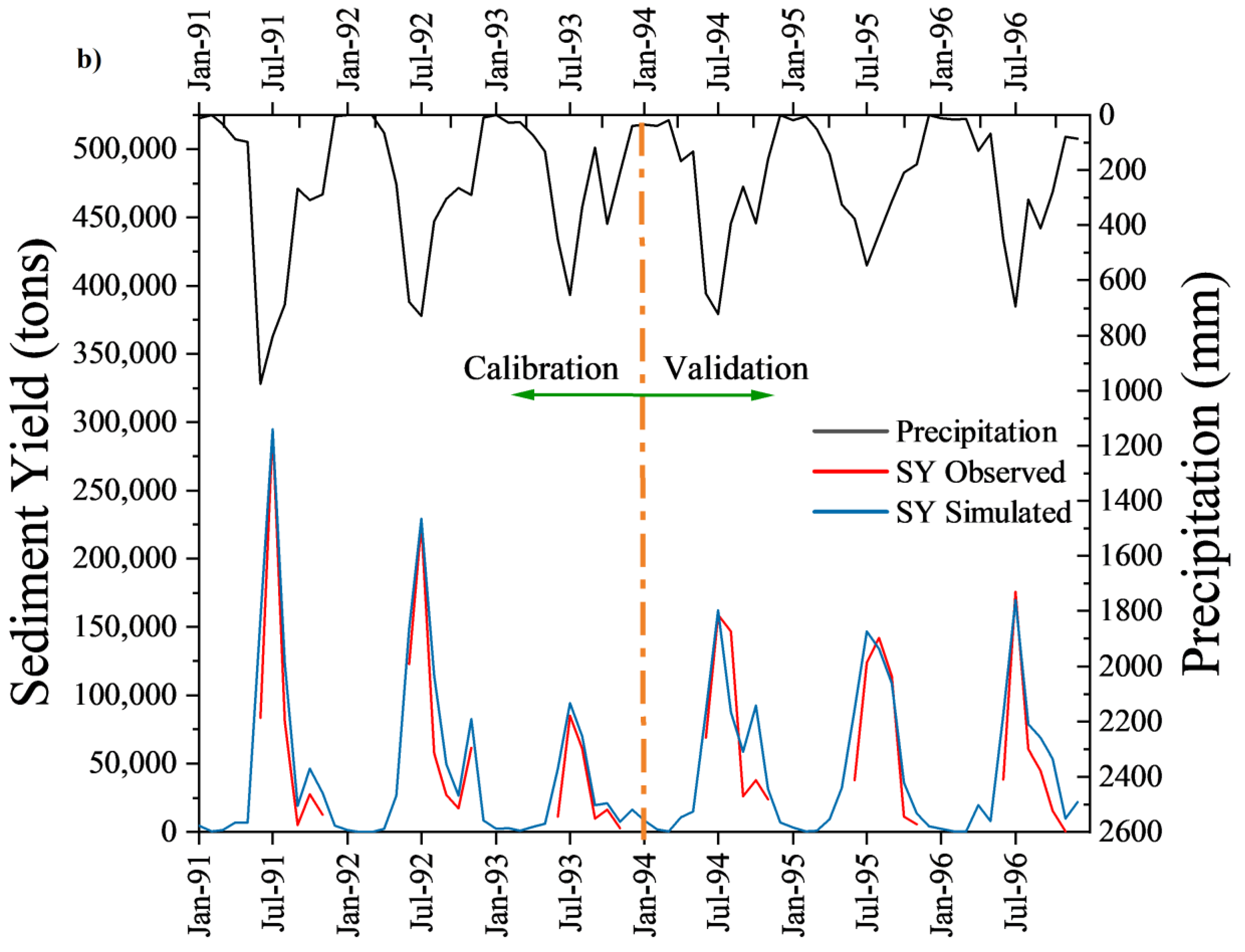
3.2. Calibration and Validation of the PRW SWAT Model

The SWAT model set up for PRW divided the watershed into 27 sub-watersheds (Figure 1b). The model was calibrated for streamflow and sediment yield at the watershed outlet (Neeleshwaram gauging station; outlet of sub-watershed #8)) for the years 1991–2004. The model performance was evaluated by comparing the model outputs with observed streamflow and sediment data. The calibrated SWAT model parameters and their adjusted values for PRW are shown in

Table 2. Sensitivity analysis of streamflow and sediment yield calibration parameters for PRW.

	Parameter	Description	Process	Fitted Value	Rank
Surface runoff	CN2.mgt	initial SCS-CN II value	Surface runoff	−0.010 (r)	1
	ALPHA_BNK.rte	baseflow alpha factor for bank storage	Channel	0.063 (v)	2
	SOL_AWC.sol	available water capacity of the soil layer	Soil water	0.274 (v)	3
	ESCO.hru	soil evaporation compensation factors	Evapotranspiration	−0.062 (r)	4
	ALPHA_BF.gw	base flow alpha factor (day)	Groundwater	0.0049 (v)	5
	GW_DELAY.gw	groundwater delay (days)	Groundwater	125.04 (v)	6
	SURLAG.bsn	surface runoff lag time (days)	Surface runoff	19.067 (v)	7
	GW_REVAP.gw	groundwater revap coefficient	Groundwater	0.029 (v)	8
Sedimentation	LAT_SED.hru	sediment concentration in lateral and groundwater flow	erosion	12.57 (v)	1
	USLE_P.sol	USLE support practice factor	Management parameter	0.32 (r)	2
	USLE_K.sol	USLE soil erodibility factor	Management parameter	−0.574 (r)	3
	SLSSUBBSN.hru	average slope length	Topographic character-istics	0.0056 (r)	4

. For streamflow, the most sensitive parameters, in order, were SCS-CN II value (CN2), baseflow alpha factor for bank storage (ALPHA_BNK), the available water capacity of the soil layer for plant uptake (SOL_AWC), soil evaporation compensation factors (ESCO), base flow recession constant (ALPHA_BF), groundwater delay (GW_DELAY), surface runoff lag time (SURLAG), and groundwater revap (percolation) coefficient (GW_REVAP). The sensitivity analysis shows that CN2 and ALPHA_BNK were the most sensitive parameters. CN2 varies in accordance with land cover, soil permeability, and antecedent moisture conditions. It controls the runoff (directly proportional) simulated after precipitation, and this runoff significantly controls the streamflow in the river channel. ALPHA_BNK controls the bank storage in a sub-basin, which contributes to river flow and reaches within the sub-basin. Return flow from bank storage is an important process that contributes significant proportions of baseflow to large rivers [53]. SOL_AWC varies with soil type (more for loam and clay) and strongly influences the percolation, evaporation, and lateral flow [50]. ESCO controls the soil evaporation demand from the soil layer. Evaporation demand directly influences runoff and flow rate. ALPHA_BF is a direct indicator of groundwater flow (base flow) response to changes in recharge. GW_DELAY controls the delay time in aquifer recharge after water moves from the soil to the main channel. This significantly increases the flow rates. In large sub-basins, with the time of concentration of more than 1 day, only a portion of surface runoff reaches the main channel on the day of generation. SURLAG contributes to managing this lag in surface runoff and sedimentation. GW_REVAP controls the movement of water into overlying unsaturated layers as a function of evaporation water demand. This process is significant in watersheds where the saturated zone is near the surface or where deep-rooted plants are growing [50].

For calibration of soil erosion and sedimentation, the most sensitive parameters were the sediment concentration in lateral and groundwater flow (LAT_SED), universal soil loss equation (USLE), soil erodibility factor (USLE_K), USLE support practice factor (USLE_P), and average slope length (SLSSUBBSN). Similar results are identified for sensitivity analysis in other studies in the literature [11,22,54].

The goodness of fit was tested using the coefficient of determination (R²), Nash–Sutcliffe efficiency (NSE) [55], percent bias (PBIAS) [56], and RMSE-observations-to-standard-deviation ratio (RSR) [57]. Streamflow calibration efforts achieved an R² and NSE of 0.86 and 0.81 during the calibration period (1991–1998), and 0.84 and 0.80 during the validation period (1999–2004), respectively. Additionally, PBIAS and RSR values were +6.5% and 0.38 for the calibration period (1991–1998) and +8.7% and 0.46 for the validation period (1999–2004), respectively. Although the observed streamflow data for the dry season (December through May) were unavailable for comparison with the simulated outputs from 1991 to 1998, they showed a good correlation in later years (Figure 4a).

For sediment yield analysis, due to limited data availability, the calibration and validation periods used were 1991–1993 and 1994–1996, respectively (Figure 4b). During calibration, the R² and NSE were 0.79 and 0.57, whereas during the validation period, these were 0.69 and 0.51, respectively. Additionally, PBIAS and RSR values were −3.6% and 0.41 during calibration and −7.0% and 0.59 during the validation period, respectively. The resulting values of the performance indicators fall within the satisfactory range as suggested by Moriasi et al. 2007 [57], and thus the model can be considered well-calibrated for flow generation and sediment yield for scenario analyses.

3.3. LULC Change Impact on Streamflow and Sediment Yield

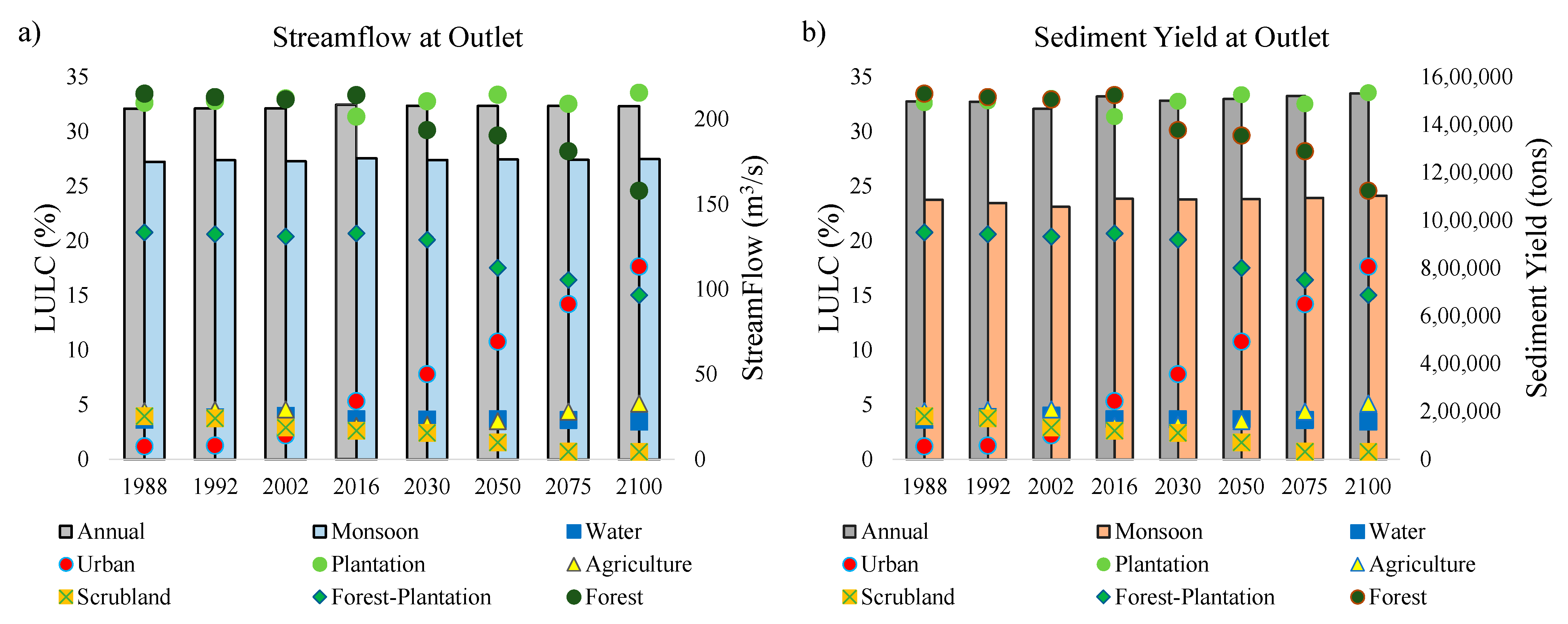
3.3.1. Effect of LULC Change at Watershed Outlet

The calibrated PRW SWAT model was executed with varying LULC scenarios to analyze the effects of LULC change on flow and sediment yield.

Table 3. Annual and monsoon SF and SY at the watershed outlet with varying LULC between 1988 and 2100.

			LULC
		1988	1992	2002	2016	2030	2050	2075	2100
Streamflow	Annual	206.21	206.33	206.54	208.61	207.98	207.96	208.06	207.81
(m3/s)	Monsoon	175.02	175.87	175.38	176.97	175.98	176.41	176.13	176.59
Sediment	Annual	14.97	14.95	14.67	15.18	14.99	15.07	15.19	15.31
Yield (×105 tons)	Monsoon	10.86	10.72	10.56	10.91	10.87	10.83	10.88	11.03

and Figure 5 show the annual and monsoon seasonal variation in SF and SY due to changes in LULC between 1988 and 2100. The year 1988 was selected as a baseline for which the average annual streamflow at the outlet was 206.21 m³/s. The results are depicted in Table 3 and Figure 5. There was no significant change in streamflow at the watershed outlet; only a minimal effect was observed, which ranged from an increase of 0.05% to 2.0% from the baseline between all LULC scenarios.

The effect of LULC change on the average annual sediment yield (SY) at the outlet was examined using 1988 as a baseline, which was 1497,111 tons. This LULC change for 1992, 2002, and 2016 resulted in minor changes in overall SY ranging from −2.05% to +1.38% from the baseline, respectively. Similarly, for LULC in 2030, 2050, 2075, and 2100, the SY at the outlet increased from 0.189% to 2.27%. The impact only during monsoon season followed a similar pattern (see Figure 5). Overall, the impact at the outlet was found to be insignificant due to the heterogeneous nature of the watershed.

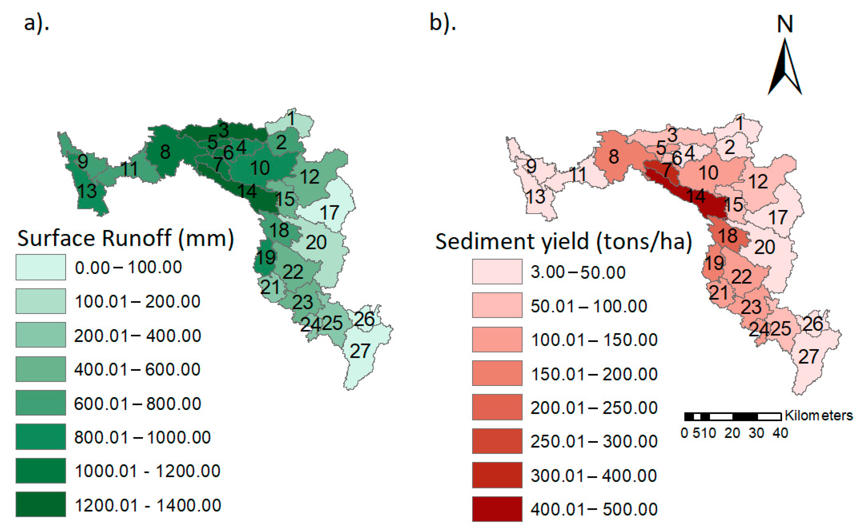
3.3.2. Effect of LULC Change at Sub-Watershed Level

The average annual and monsoon data for the years 1991–2004 were considered as the baseline (Figure 6). LULC significantly affects the runoff in a region and runoff is a major component of streamflow. Thus, the effect of LULC change on surface runoff was analyzed at the individual sub-watershed level. The spatial variation in surface runoff and sediment yield (SY) due to LULC change across the PRW for each sub-watershed is depicted in Figure 7. The average annual surface runoff values ranged from 71.26 mm (sub-watershed 26) to 1338.72 mm (sub-watershed 16). The next highest surface runoff value was 1241.08 mm for sub-watershed 3. Regions with high surface runoff (>1000 mm) included sub-watersheds 14, 8, 7, 6, and 5, whereas regions with low surface runoff (<200 mm) included sub-watersheds 27, 17, 20, and 1. Similarly, for SY, the average annual SY ranged between 3 tons/ha (sub-watershed 9) and 462.72 tons/ha (sub-watershed 16). The next highest SY was 424.95 tons/ha in sub-watershed 14. Regions with a high SY (>200 tons/ha) were sub-watersheds 16, 14, 7, and 18, whereas regions with a low SY (<50 tons/ha) were watersheds 4, 2, 1, 20, 26, 11, 27, 17, 19, and 9. It was observed that there was a positive correlation between surface runoff and SY in sub-watersheds 14, 8, 7, 6, and 18. However, it was interesting to note that sub-watersheds 2, 9, 13, and 4 showed otherwise. Two reasons were identified for such behavior, namely, high forest and plantation cover (predominantly >70%) and low slope (<8%). Sub-watersheds 2, 9, and 4 had the above combination except in the case of sub-watershed 13 (Figure 3). In sub-watershed 13, the forest and plantation cover were less than 40%, but the reason for the low SY was high water cover (>35%). For high SY, it was observed that these regions had significant scrubland cover, which contributed to sedimentation along with a high slope (>8%). Although it was noticed that some of the sub-watersheds (14, 7, 6, and 18) with a high SY had higher forest and plant cover, greater slope and scrubland presence were still the dominant factors. Additionally, it was observed that sub-watersheds at the central region and downstream end had high flows, and upstream sub-watersheds experienced low flows. The central region had the highest sediment yield.

The maximum increase in surface runoff was observed as 56.6% for 2100 at sub-watershed 3 (from 836.8 mm to 1310 mm), whereas the maximum decrease of 14.56% was seen for 2100 at sub-watershed 23 (from 404.03 mm to 345.19 mm). From 1988 to 2100, an increase was observed in surface runoff in most of the sub-watersheds (Figure 7). This can be attributed to the decrease in forest and plantation cover and increase in urban area (Figure 3). Similarly, for SY, most of the sub-watersheds showed a decrease in SY. The main reason attributed to this is the reduction in scrubland area, which is identified as the primary contributor to SY. However, a major part of this scrubland was converted into urban area, which led to an increase in surface runoff but a negative effect of SY as no free soil was available to erode. The sub-watersheds showing a high increase in SY were either near the downstream end (sub-watershed 9) or at high elevation (sub-watersheds 2 and 4). Thus, it becomes interesting to discuss certain specific sub-watershed changes for their unique variations. For instance, sub-watershed 9 is predicted to see an increase in surface runoff and SY from 1988 to 2100 (Figure 7). The increase in urban cover and reduction in plantation cover accounts for the increased surface runoff, whereas an increase in agriculture augmented with flash flow due to urbanization explains the high SY (Figure 3). Similar to sub-watershed 9, sub-watershed 8 also had a similar combination of LULC changes, but the difference observed here was a reduction in scrubland, which results in low SY, whereas high surface runoff was still observed. This clearly indicates that SY is more dependent on the availability of scrubland than other LULC transitions. Sub-watershed 11 also showed similar changes to those of sub-watershed 9.

Sub-watershed 13 also showed its unique combination of LULC variations where despite the increase in surface runoff, there was a reduction in SY till 2100 (Figure 7). Here, no scrubland was available to alter the changes in SY. However, the reduction in plantation and agricultural area suggests it is a significant reason for SY reduction (Figure 3). However, these LULC classes were converted into urban spaces, which resulted in the reduction in loose surfaces for erosion. Similar indications were learned from observations in the case of sub-watersheds 8 and 9. In addition to this, the presence of water bodies (>35%) in sub-watershed 13 contributed to low SY. Sub-watershed 19 was also similar to 13, but here no urban transition was present. Instead, changes in scrubland dominated over other changes and controlled the SY (Figure 3 and Figure 7).

Other than this, several watershed combinations (1,2, 4, and 5) and (19, 21 21, 22, and 23) followed the same trend in changes in surface runoff and SY. The common outcome of all these transitions was, in the case of surface runoff, an increase in urbanization that dominated over a reduction in forest/plantation cover and then a reduction in agriculture area, leading to high surface runoff. In the case of SY, a reduction in scrubland followed by a reduction in agriculture followed by the transition to urban cover followed by the presence of a water body led to reduced SY. Further, in the case of nominal change (<1%) in LULC, no/insignificant change was observed in surface runoff or SY, as observed in sub-watersheds 24 (2050 to 2100), 25 (2050 to 2100), 26 (2050 to 2100), and 27(2002 to 2030).

4. Discussion

Human activities are the primary drivers of dynamic changes in land use and land cover. The expansion of settlements and the population will necessitate more living space, which may result in a decrease in vegetated areas. The continuous demand for space and other natural resources may lead to people shifting to and settling in forested areas, resulting in forest degradation and increased surface runoff. It is a well-recognized fact that the effects of a change in LULC are minimal when viewed as a whole across space and time [9,10], whereas at the sub-basin scale, the impact of dynamic land use change on the hydrological response became more apparent [11]. In a monsoon-dominated region, flow and sediment yield are the factors most significantly affected by LULC changes, and the study of these characteristics at the sub-watershed scale provides more insights about these effects.

The results for LULC change impact on streamflow (SF), surface runoff, and sediment yield (SY) in the Periyar River Watershed (PRW) provide so many insights into the governing factors that control the flow properties in a monsoon-dominated watershed. Different combinations of LULC transition affect the watershed hydrology differently and can result in small widespread changes in the watershed [9,10,54]. Thus, in this study, special focus was given to analysis at the sub-watershed scale along with identifying changes at watersheds. The analysis of the monthly time step at the watershed scale indicates that the streamflow and sediment yield at the outlet were very low despite the high increase in urbanization, change in agriculture area, and change in plantation and/or forest cover leading up to 2100. However, greater insights were gained regarding the various combinations of LULC changes that affect surface runoff and SY when studied at the sub-catchment scale. Urbanization is identified as a major reason for increases in surface runoff. Other factors include a reduction in plantation/forest cover and high slope, which result in higher surface runoff. These results are in consensus with studies conducted in other regions [11,12,22,27,54]. For example, Aghsaei et al. (2020) [11] found that urbanization reduced evapotranspiration (ET) and increased surface runoff in the Anzali Wetland, Iran. Dynamic LULC change had a minimal effect on sediment yield for the entire catchment. Additionally, Kundu et al. (2017) [27] suggested that increasing agricultural land increases water demand, which decreases ET. Similar trends are also observed in the PRW. However, the prioritization of each transition was identified by comparing the changes at the sub-watershed scale. Similarly, for SY, scrubland cover, agricultural land, and water body cover were identified as major factors. For instance, higher slope [22,58], high precipitation and/or streamflow [21,22,54], and the presence of agricultural area [12,22] lead to high sediment yield in specific conditions.

The analysis and results for each individual sub-watershed were very useful in identifying the key factors controlling flow in consideration of LULC. In this context, an understanding of how LULC affects streamflow, surface runoff, and sediment output at watershed and sub-watershed scales in a monsoon-dominated humid tropical region of India is highly useful. Furthermore, the LULC change trend showed that there was an increase in urbanization. The urban growth was concentrated in a few sub-watersheds (8, 9, 11, and 13, refer to Figure 2). These are the areas in close proximity to the water bodies. This indicates that there is a chance of increasing water stress in the future, and special attention must be given to these areas.

5. Conclusions

The present study focused on identifying the role of LULC change on the streamflow (SF) and sediment yield (SY) in a monsoon-dominated region at watershed and sub-watershed scales. To achieve this, the SWAT hydrological model was set up for the Periyar River Watershed, and the model was run with varying LULC data from 1988 to 2100. The trend of classified historical maps was used for projecting the future LULC. Between 1988 and 2016, the urban area increased by 4.13%, while plantation and forest coverage decreased by 1.5%. At this rate, by 2100, urban areas are expected to grow by 16.45% while plantations and forest will shrink by 13.7%. The effects of these changes on SF and SY were found to be minimal at the watershed outlet; however, at the spatial scale of sub-watersheds, the changes varied by up to 70% for surface runoff and 200% for SY. The analysis at the sub-watershed scale provided insights that show the variation in surface runoff and SY is not only governed by LULC change but is a combination of several other parameters, such as slope, elevation, and soil properties. The analysis at the sub-watershed scale highlighted the effect of various combinations of LULC change on surface runoff and SY. Scrubland’s significant contribution to high SY was noticed in all sub-watersheds. Further, areas with high agricultural cover are expected to show greater SY, although this might not be true in the case of flat terrain. Thus, these factors, along with several other combinations, were the highlights of this study. The analysis shows the importance of considering detailed LULC analysis in watershed management practices for sustainable development. These results will be beneficial in designing watershed management policies. It is recommended that the proposed approach be used in other watersheds with variable climatic conditions (e.g., arid, semi-arid, mountainous, etc.) to analyze the effect of LULC change on the hydrological regime at the sub-watershed scale in different climatic complexities.

References

1. Anand, J.; Gosain, A.K.; Khosa, R. Prediction of land use changes based on Land Change Modeler and attribution of changes in the water balance of Ganga basin to land use change using the SWAT model. Sci. Total Environ. 2018, 644, 503–519. [Google Scholar] [CrossRef] [PubMed]
2. Stonestrom, D.A.; Scanlon, B.R.; Zhang, L. Introduction to special section on Impacts of Land Use Change on Water Resources. Water Resour. Res. 2009, 45, 2–4. [Google Scholar] [CrossRef] [Green Version]
3. Shi, P.-J.; Yuan, Y.; Zheng, J.; Wang, J.-A.; Ge, Y.; Qiu, G.-Y. The effect of land use/cover change on surface runoff in Shenzhen region, China. CATENA 2007, 69, 31–35. [Google Scholar] [CrossRef]
4. Hwang, S.-A.; Hwang, S.-J.; Park, S.-R.; Lee, S.-W. Examining the Relationships between Watershed Urban Land Use and Stream Water Quality Using Linear and Generalized Additive Models. Water 2016, 8, 155. [Google Scholar] [CrossRef] [Green Version]
5. Li, P.; Li, H.; Yang, G.; Zhang, Q.; Diao, Y. Assessing the Hydrologic Impacts of Land Use Change in the Taihu Lake Basin of China from 1985 to 2010. Water 2018, 10, 1512. [Google Scholar] [CrossRef] [Green Version]
6. Dwarakish, G.S.; Ganasri, B.P. Impact of land use change on hydrological systems: A review of current modeling approaches. Cogent Geosci. 2015, 1, 1115691. [Google Scholar] [CrossRef]
7. Elfert, S.; Bormann, H. Simulated impact of past and possible future land use changes on the hydrological response of the Northern German lowland ‘Hunte’ catchment. J. Hydrol. 2010, 383, 245–255. [Google Scholar] [CrossRef]
8. Mao, D.; Cherkauer, K.A. Impacts of land-use change on hydrologic responses in the Great Lakes region. J. Hydrol. 2009, 374, 71–82. [Google Scholar] [CrossRef]
9. Wagner, P.D.; Kumar, S.; Fiener, P.; Schneider, K. Technical Note: Hydrological Modeling with SWAT in a Monsoon-Driven Environment: Experience from the Western Ghats, India. Trans. ASABE 2011, 54, 1783–1790. [Google Scholar] [CrossRef]
10. Fohrer, N.; Haverkamp, S.; Eckhardt, K.; Frede, H.-G. Hydrologic Response to land use changes on the catchment scale. Phys. Chem. Earth Part B Hydrol. Ocean. Atmos. 2001, 26, 577–582. [Google Scholar] [CrossRef]
11. Aghsaei, H.; Dinan, N.M.; Moridi, A.; Asadolahi, Z.; Delavar, M.; Fohrer, N.; Wagner, P.D. Effects of dynamic land use/land cover change on water resources and sediment yield in the Anzali wetland catchment, Gilan, Iran. Sci. Total Environ. 2020, 712, 136449. [Google Scholar] [CrossRef] [PubMed]
12. Schilling, K.E.; Jha, M.K.; Zhang, Y.K.; Gassman, P.W.; Wolter, C.F. Impact of land use and land cover change on the water balance of a large agricultural watershed: Historical effects and future directions. Water Resour. Res. 2008, 44, 1–12. [Google Scholar] [CrossRef]
13. Samal, D.R.; Gedam, S. Assessing the impacts of land use and land cover change on water resources in the Upper Bhima river basin, India. Environ. Chall. 2021, 5, 100251. [Google Scholar] [CrossRef]
14. Leta, M.K.; Demissie, T.A.; Tränckner, J. Hydrological Responses of Watershed to Historical and Future Land Use Land Cover Change Dynamics of Nashe Watershed, Ethiopia. Water 2021, 13, 2372. [Google Scholar] [CrossRef]
15. Dixon, B.; Earls, J. Effects of urbanization on streamflow using SWAT with real and simulated meteorological data. Appl. Geogr. 2012, 35, 174–190. [Google Scholar] [CrossRef]
16. Lin, B.; Chen, X.; Yao, H.; Chen, Y.; Liu, M.; Gao, L.; James, A. Analyses of landuse change impacts on catchment runoff using different time indicators based on SWAT model. Ecol. Indic. 2015, 58, 55–63. [Google Scholar] [CrossRef]
17. Öztürk, M.; Copty, N.K.; Saysel, A.K. Modeling the impact of land use change on the hydrology of a rural watershed. J. Hydrol. 2013, 497, 97–109. [Google Scholar] [CrossRef]
18. Aichele, S.S. Effects of Urban Land-Use Change on Streamflow and Water Quality in Oakland County, Michigan, 1970–2003, as Inferred from Urban Gradient and Temporal Analysis: U.S. Geological Survey Scientific Investigations Report 2005–5016. 22p. Available online: https://pubs.usgs.gov/sir/2005/5016/pdf/SIR2005-5016.pdf (accessed on 13 October 2022).
19. Miao, C.Y.; Yang, L.; Chen, X.H.; Gao, Y. The vegetation cover dynamics (1982-2006) in different erosion regions of the Yellow River Basin, China. L. Degrad. Dev. 2012, 23, 62–71. [Google Scholar] [CrossRef]
20. Babel, M.S.; Gunathilake, M.B.; Jha, M.K. Evaluation of Ecosystem-Based Adaptation Measures for Sediment Yield in a Tropical Watershed in Thailand. Water 2021, 13, 2767. [Google Scholar] [CrossRef]
21. Sinha, R.K.; Eldho, T.I. Effects of historical and projected land use/cover change on runoff and sediment yield in the Netravati river basin, Western Ghats, India. Environ. Earth Sci. 2018, 77, 111. [Google Scholar] [CrossRef]
22. de Oliveira Serrão, E.A.; Silva, M.T.; Ferreira, T.R.; de Ataide LC, P.; dos Santos, C.A.; de Lima AM, M.; da Silva, V.d.P.R.; de Sousa, E.d.A.S.; Gomes, D.J.C. Impacts of land use and land cover changes on hydrological processes and sediment yield determined using the SWAT model. Int. J. Sediment Res. 2022, 37, 54–69. [Google Scholar] [CrossRef]
23. Rogger, M.; Agnoletti, M.; Alaoui, A.; Bathurst, J.C.; Bodner, G.; Borga, M.; Chaplot, V.; Gallart, F.; Glatzel, G.; Hall, J.; et al. Land use change impacts on floods at the catchment scale: Challenges and opportunities for future research. Water Resour. Res. 2017, 53, 5209–5219. [Google Scholar] [CrossRef] [PubMed] [Green Version]
24. Chen, Q.; Chen, H.; Zhang, J.; Hou, Y.; Shen, M.; Chen, J.; Xu, C. Impacts of climate change and LULC change on runoff in the Jinsha River Basin. J. Geogr. Sci. 2020, 30, 85–102. [Google Scholar] [CrossRef] [Green Version]
25. Chang, H.; Franczyk, J. Climate change, land-use change, and floods: Toward an integrated assessment. Geogr. Compass 2008, 2, 1549–1579. [Google Scholar] [CrossRef]
26. Wheater, H.; Evans, E. Land use, water management and future flood risk. Land use policy 2009, 26, S251–S264. [Google Scholar] [CrossRef]
27. Kundu, S.; Khare, D.; Mondal, A. Past, present and future land use changes and their impact on water balance. J. Environ. Manage. 2017, 197, 582–596. [Google Scholar] [CrossRef]
28. Leta, O.; Bauwens, W. Assessment of the Impact of Climate Change on Daily Extreme Peak and Low Flows of Zenne Basin in Belgium. Hydrology 2018, 5, 38. [Google Scholar] [CrossRef] [Green Version]
29. Shahid, M.; Rahman, K.U.; Haider, S.; Gabriel, H.F.; Khan, A.J.; Pham, Q.B.; Pande, C.B.; Linh, N.T.; Anh, D.T. Quantitative assessment of regional land use and climate change impact on runoff across Gilgit watershed. Environ. Earth Sci. 2021, 80, 743. [Google Scholar] [CrossRef]
30. Kim, J.; Choi, J.; Choi, C.; Park, S. Science of the Total Environment Impacts of changes in climate and land use/land cover under IPCC RCP scenarios on stream fl ow in the Hoeya River Basin, Korea. Sci. Total Environ. 2013, 452, 181–195. [Google Scholar] [CrossRef] [PubMed]
31. Sinha, R.K.; Eldho, T.I.; Subimal, G. Assessing the impacts of land use/land cover and climate change on surface runoff of a humid tropical river basin in Western Ghats, India. Int. J. River Basin Manag. 2020, 1–12. [Google Scholar] [CrossRef]
32. Köppen, W. Grundriß der Klimakunde; De Gruyter: Berlin, Germany, 1931; Volume 20. [Google Scholar] [CrossRef]
33. Beck, H.E.; Zimmermann, N.E.; McVicar, T.R.; Vergopolan, N.; Berg, A.; Wood, E.F. Present and future Köppen-Geiger climate classification maps at 1-km resolution. Sci. Data 2018, 5, 180214. [Google Scholar] [CrossRef] [PubMed] [Green Version]
34. CWC. Kerala Floods of August 2018. Central Water Commission, New Delhi. 2018. Available online: https://sdma.kerala.gov.in/wp-content/uploads/2020/10/Kerala_28122018_CWC_December-2018.pdf (accessed on 1 March 2020).
35. Sudheer, K.P.; Bhallamudi, S.M.; Narasimhan, B.; Thomas, J.; Bindhu, V.M.; Vema, V.; Kurian, C. Role of dams on the floods of August 2018 in Periyar River Basin, Kerala. Curr. Sci. 2019, 116, 780–794. [Google Scholar] [CrossRef]
36. Mohanakrishnan, A.; Verma, C.V.J. History of the Periyar Dam with Century Long Performance; Central Board of Irrigation & Power: New Delhi, India, 1997. [Google Scholar]
37. Patil, A.; Ramsankaran, R.A.A.J. Improved streamflow simulations by coupling soil moisture analytical relationship in EnKF based hydrological data assimilation framework. Adv. Water Resour. 2018, 121, 173–188. [Google Scholar] [CrossRef]
38. Ganguli, P.; Singh, B.; Reddy, N.N.; Raut, A.; Mishra, D.; Das, B.S. Climate-catchment-soil control on hydrological droughts in peninsular India. Sci. Rep. 2022, 12, 8014. [Google Scholar] [CrossRef]
39. Pai, D.S.; Rajeevan, M.; Sreejith, O.P.; Mukhopadhyay, B.; Satbha, N.S. Development of a new high spatial resolution (0.25° × 0.25°) long period (1901–2010) daily gridded rainfall data set over India and its comparison with existing data sets over the region. MAUSAM 2014, 65, 1–18. [Google Scholar] [CrossRef]
40. Srivastava, A.K.; Rajeevan, M.; Kshirsagar, S.R. Development of a high resolution daily gridded temperature data set (1969-2005) for the Indian region. Atmos. Sci. Lett. 2009, 10, 249–254. [Google Scholar] [CrossRef]
41. Lu, D.; Weng, Q. A survey of image classification methods and techniques for improving classification performance. Int. J. Remote Sens. 2007, 28, 823–870. [Google Scholar] [CrossRef]
42. Liping, C.; Yujun, S.; Saeed, S. Monitoring and predicting land use and land cover changes using remote sensing and GIS techniques—A case study of a hilly area, Jiangle, China. PLoS ONE 2018, 13, e0200493. [Google Scholar] [CrossRef]
43. Ullah, K.; Zhang, J. GIS-based flood hazard mapping using relative frequency ratio method: A case study of panjkora river basin, eastern Hindu Kush, Pakistan. PLoS ONE 2020, 15, e0229153. [Google Scholar] [CrossRef]
44. Manandhar, R.; Odehi, I.O.A.; Ancevt, T. Improving the accuracy of land use and land cover classification of landsat data using post-classification enhancement. Remote Sens. 2009, 1, 330–344. [Google Scholar] [CrossRef] [Green Version]
45. Muller, M.R.; Middleton, J. A Markov model of land-use change dynamics in the Niagara Region, Ontario, Canada. Landsc. Ecol. 1994, 9, 151–157. [Google Scholar]
46. Adhikari, S.; Southworth, J. Simulating forest cover changes of bannerghatta national park based on a CA-Markov model: A remote sensing approach. Remote Sens. 2012, 4, 3215–3243. [Google Scholar] [CrossRef] [Green Version]
47. Marhaento, H.; Booij, M.J.; Hoekstra, A.Y. Attribution of changes in stream flow to land use change and climate change in a mesoscale tropical catchment in Java, Indonesia. Hydrol. Res. 2017, 48, 1143–1155. [Google Scholar] [CrossRef]
48. Arnold, J.G.; Srinivasan, R.; Muttiah, R.S.; Williams, J.R. Large area hydrologic modeling and assessment part i: Model development. J. Am. Water Resour. Assoc. 1998, 34, 73–89. [Google Scholar] [CrossRef]
49. Arnold, J.G.; Williams, J.R.; Maidment, D.R. Continuous-Time Water and Sediment-Routing Model for Large Basins. J. Hydraul. Eng. 1995, 121, 171–183. [Google Scholar] [CrossRef]
50. Neitsch, S.L.; Arnold, J.G.; Kiniry, J.R.; Williams, J.R. Soil and Water Assessment Tool Theoretical Documentation Version 2009; Texas Water Resources Institute: College Station, TX, USA, 2011.
51. Wannasin, C.; Brauer, C.C.; Uijlenhoet, R.; van Verseveld, W.J.; Weerts, A.H. Daily flow simulation in Thailand Part I: Testing a distributed hydrological model with seamless parameter maps based on global data. J. Hydrol. Reg. Stud. 2021, 34, 100794. [Google Scholar] [CrossRef]
52. Jha, M.; Gassman, P.W.; Secchi, S.; Gu, R.; Arnold, J. Effect of watershed subdivision on swat flow, sediment, and nutrient predictions. J. Am. Water Resour. Assoc. 2004, 40, 811–825. [Google Scholar] [CrossRef] [Green Version]
53. Duvert, C.; Lim, H.S.; Irvine, D.J.; Bird, M.I.; Bass, A.M.; Tweed, S.O.; Hutley, L.B.; Munksgaard, N.C. Hydrological processes in tropical Australia: Historical perspective and the need for a catchment observatory network to address future development. J. Hydrol. Reg. Stud. 2022, 43, 101194. [Google Scholar] [CrossRef]
54. Sinha, R.K.; Eldho, T.I.; Ghosh, S. Assessing the impacts of land cover and climate on runoff and sediment yield of a river basin. Hydrol. Sci. J. 2020, 65, 2097–2115. [Google Scholar] [CrossRef]
55. Legates, D.R.; McCabe, G.J. Evaluating the use of ‘goodness-of-fit’ measures in hydrologic and hydroclimatic model validation. Water Resour. Res. 1999, 35, 233–241. [Google Scholar] [CrossRef]
56. Gupta, H.V.; Sorooshian, S.; Yapo, P.O. Status of Automatic Calibration for Hydrologic Models: Comparison with Multilevel Expert Calibration. J. Hydrol. Eng. 1999, 4, 135–143. [Google Scholar] [CrossRef]
57. Moriasi, D.N.; Arnold, J.G.; van Liew, M.W.; Bingner, R.L.; Harmel, R.D.; Veith, T.L. Model Evaluation Guidelines for Systematic Quantification of Accuracy in Watershed Simulations. Trans. ASABE 2007, 50, 885–900. [Google Scholar] [CrossRef]
58. Kothyari, U.C. Erosion and sedimentation problems in India. IAHS-AISH Publ. 1996, 236, 531–540. [Google Scholar]
Figure 1. (a) Location, (b) delineated sub-watersheds (with sub-watersheds numbered from 1 to 27), (c) soil texture, (d) elevation map, and (e) average monthly precipitation (1991–2004) for PRW.
Water 14 03666 g001
Figure 2. Classified: (a) 1988, (b) 1992, (c) 2002, (d) 2016; projected: (e) 2016, (f) 2030, (g) 2050, (h) 2075; (i) 2100 LULC maps for PRW; (j) percentage change in LULC classes (1988–2100).
Water 14 03666 g002
Figure 3. LULC change (%) in sub-basins of PRW for the years 1988, 1992, 2002, 2016, 2030, 2050, 2075, and 2100.
Water 14 03666 g003
Figure 4. Calibration and validation for (a) streamflow (1991–2004) and (b) sediment yield (1991–1996) at Neeleshwaram gauging station of PRW. Note: the streamflow data during the dry months (December through May) were not available for 1991–1998.
Water 14 03666 g004aWater 14 03666 g004b
Figure 5. Annual and monsoon season (a) streamflow and (b) sediment yield at the outlet (sub-watershed 8) with varying LULC between 1988 and 2100. Note: most of the changes in urban area occurred in the region downstream of watershed #8, so a direct impact of urban on SF and SY is not visible.
Water 14 03666 g005
Figure 6. Spatial distribution of average annual (a) surface runoff and (b) sediment yield at sub-watershed (#1 to #27) for the period 1991–2004 with LULC 1988 (baseline). (Here, # indicates the sub-watershed ID.)
Water 14 03666 g006
Figure 7. Spatial variation of change (%) in the (a) surface runoff and (b) sediment yield at sub-watershed outlet with varying LULC between 1988 and 2100 across the sub-watersheds (#1 to #27): (i) 1992-1988; (ii) 2002-1988; (iii) 2016-1988; (iv) 2030-1988; (v) 2050-1988; (vi) 2075-1988; and (vii) 2100-1988.
Water 14 03666 g007