1. Introduction
Flood discharge probabilities and their relationship with extreme rainfall probabilities is not a well-addressed subject in the literature; hence, it is a very interesting subject from both theoretical and practical perspectives. Flood design is based on extreme value analysis of observed flood peak discharges at a site. However, the measurements of flood discharges are not often available, at least not in time series of adequate lengths. For this reason, hydrologists tend to estimate design floods based on design storms [
1,
2]. Observed rainfall is used for extracting extreme values (i.e., annual maxima series approach, peak over threshold method), estimating the design rainfall of a given return period, and then, the estimated rainfall is used as an input for a rainfall–runoff model. The aforementioned approach, called the design storm method, is widely applied and has prevailed in engineering practice (e.g., [
3]), especially in urban areas where runoff data are very rarely available. The assumption of equivalent (i.e., equal) return periods of rainfall and flood flow may hold true in the case of a block rainfall with fixed duration, invariant rainfall, invariant routing, invariant discharge and a runoff coefficient that remains constant over the rainfall duration. However, in real world basins this is not the case, and the return period of rainfall is not the same as the return period of peak discharge. As a result, researchers have raised concerns regarding the design storm method (e.g., [
4,
5]).
Pilgrim and Cordery [
6] addressed the problem, employing the rational method, by providing runoff coefficients for which the return periods of the design storm will produce flood peaks with the same return periods as the observed ones. Alfieri et al. [
7] provided correction factor(s) for the accurate estimation of design floods. Viglione and Blöschl [
8] stated that the relation between the storm return period and flood return period is not well understood. They concluded that for storms with varying duration, the return period of floods is always greater than that of the rainfall. Breinl et al. [
5] examined the relationship between flood and rainfall return periods and proposed a novel framework for comparing (elasticity of floods to rainfall extremes) annual maxima rainfall (in the form of intensity–duration–frequency curves) with annual maximum streamflow. The proposed approach was applied in 314 rain gauges and 428 streams in Austria. Sutcliffe [
9] reported that storms with return periods of 2, 8, 17, 35, 50, 81, 140, 300, 520 and 1000 years correspond to flood flows with return periods of 2.33, 5, 10, 20, 30, 50, 100, 250, 500 and 1000 years, respectively.
The Extreme Value Theory was introduced by Gumbel [
10] and mainly involves the following steps: (i) observed flood data ordering; (ii) fitting of a theoretical distribution function and parameter estimation; and (iii) extrapolation of the tails of the distribution to large return periods (low probabilities of occurrence). Various researchers have applied extreme value analysis to estimate the probabilities of extreme flood events, rainfall events, sea levels etc. (e.g., [
11,
12,
13,
14,
15,
16,
17,
18,
19]). A wide variety of theoretical distributions have been used for rainfall and flood frequency analysis (e.g., [
20]). The most widely used distributions are: Normal (e.g., [
21]), Log-normal (e.g., [
22]), Log-normal with three parameters (e.g., [
23]), Exponential (e.g., [
24]), Two-component exponential (e.g., [
25]); Gamma (e.g., [
8]), Pearson Type III (e.g., [
26]), Log-Pearson Type III (e.g., [
27]), Extreme Value Type I (Gumbel; e.g., [
28]), Extreme Value Type II (Fréchet; e.g., [
29]), Extreme Value Type III (Weibull; e.g., [
30]), Generalized Extreme Value (GEV; e.g., [
31]), Generalized Pareto (e.g., [
32]), Generalized logistic (e.g., [
33]) and Wakeby (e.g., [
23]). Countries have adopted different theoretical distributions as standard models for flood and/or rainfall frequency analysis [
20]. For example, in the United States of America and Australia, the Log-Pearson Type III is the standard model for flood frequency analysis, while in the United Kingdom, the Generalized logistic is the standard model for extreme value analysis of floods. In Greece, the GEV theoretical distribution is the standard model for rainfall frequency analysis. For a review of recent applications of frequency analysis in the field of hydrology, the interested reader is referred to WMO [
20], Grimaldi et al. [
34] and Madsen et al. [
35].
Different approaches have been presented in the literature for the estimation of the parameters of a theoretical distribution. The most widely used approaches are [
34]: the method of moments, the method of maximum likelihood and the L-moments approach. The method of L-moments constitutes a combination of the Probability weighted moments and was standardized by Hosking [
36]. In the present work, the GEV distribution was selected for rainfall extreme value analysis with parameters estimated employing the L-Moments method, as this is the proposed method by the technical specifications in Greece. For the flood frequency analysis, two distributions were examined, namely the Extreme Value Type I (Gumbel) and the GEV with parameters estimated using the L-Moments method [
37]. The L-Moments method was preferred as it is rather simple, it characterizes efficiently the sampled data and it is not affected by the variability of the sampling approach [
36].
The aim of this study was to first apply the two above-described approaches (i.e., the design storm approach, and continuous simulation and flood frequency analysis) using satellite rainfall data; then, to relate the rainfall return periods with flood return periods derived using hydrologic/hydraulic modeling; and finally, compare the results. Comparison was performed in terms of peak discharge at the outlet of the studied basin (i.e., design storm results vs. continuous simulation and flood frequency analysis results) and in terms of flood hazard (i.e., flood extent, inundation depths and flow velocities). Flood hazard was estimated based on the results of the hydrodynamic model. To the best of our knowledge, this is one of the very few attempts (e.g., [
9]) trying to relate rainfall and flood return periods.
4. Discussion
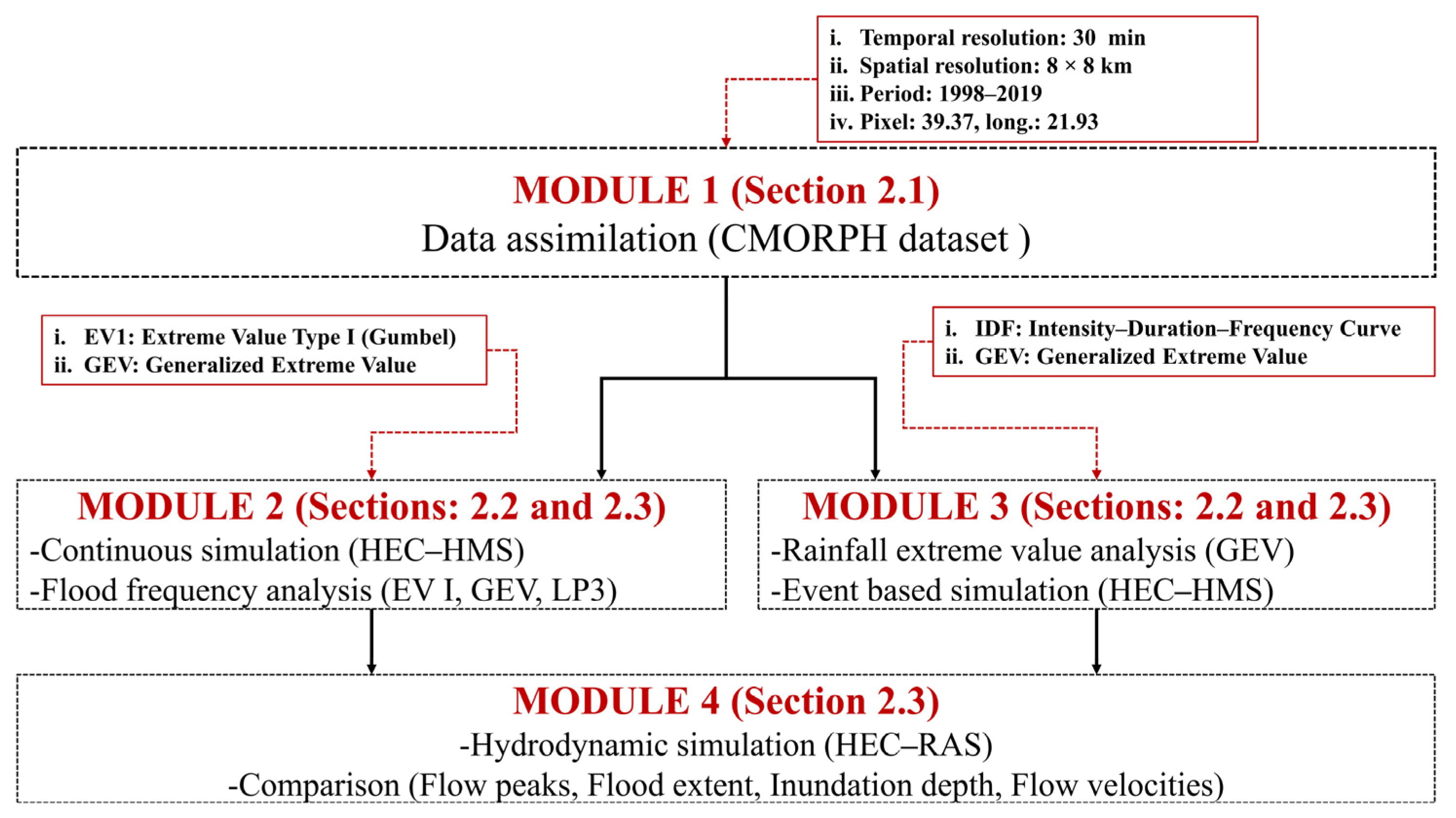
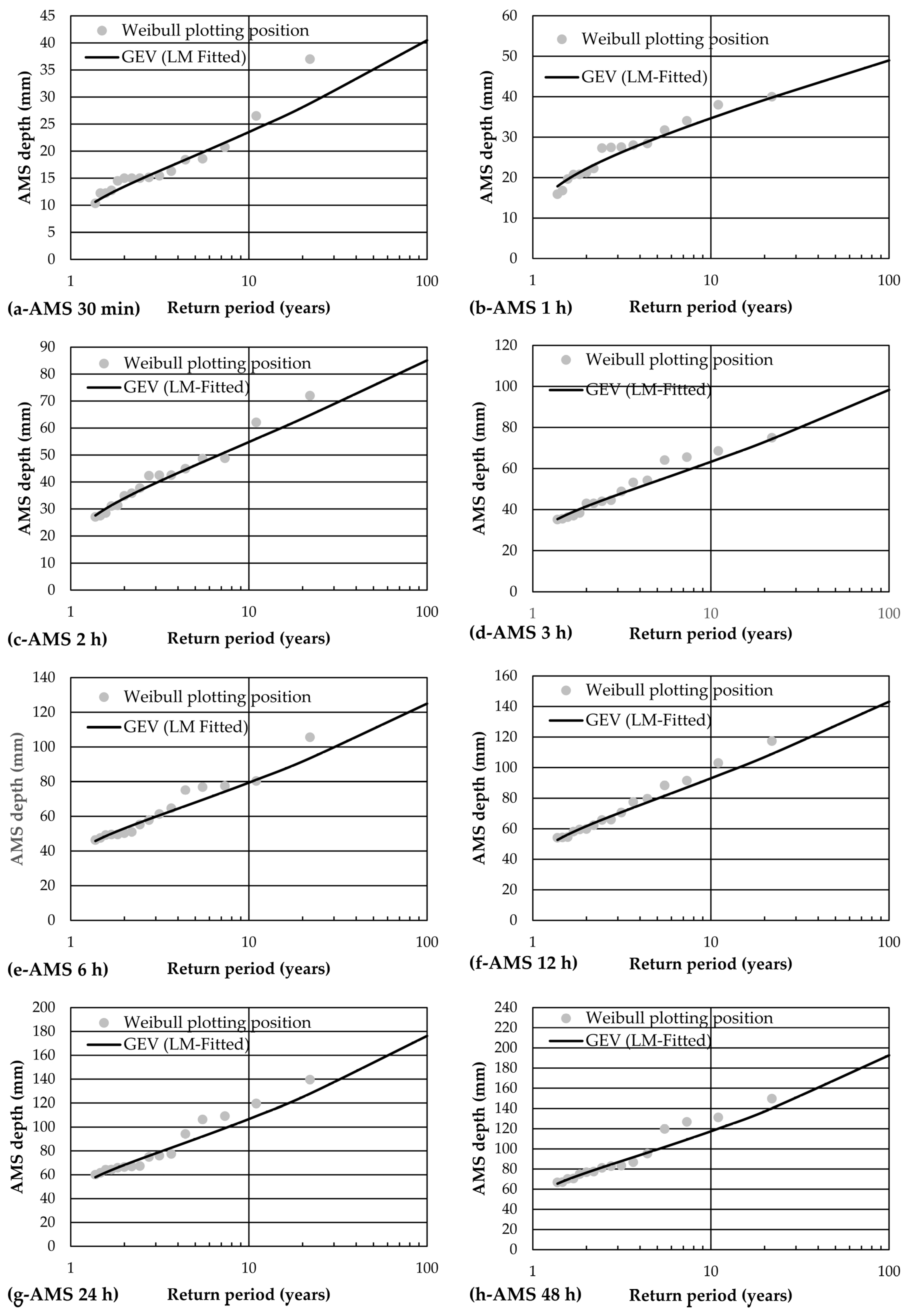
In this work, rainfall frequency analysis for developing Intensity–Duration–Frequency (IDF) curves was applied on the annual maxima rainfall using the GEV distribution, the method of L-moments for distribution fitting and the generalized approach for developing IDF curves proposed by Koutsoyiannis et al. [
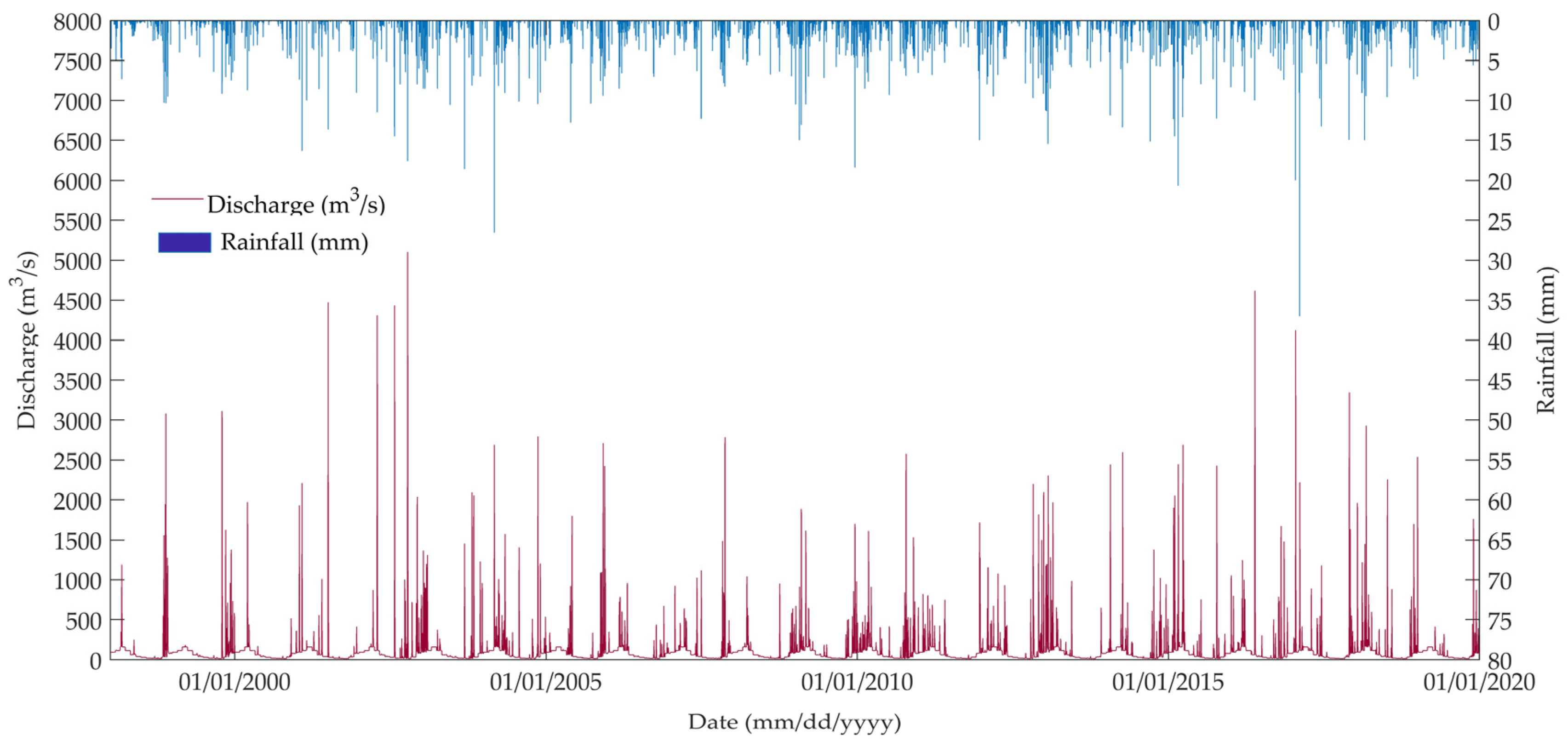
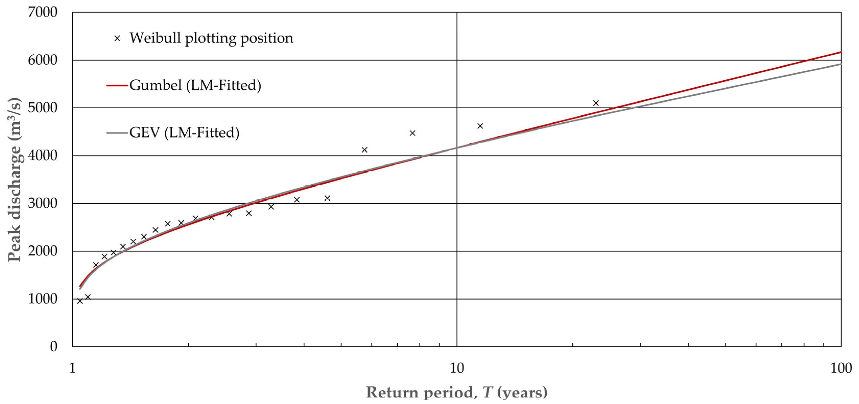
43]. The time of concentration for the basin is large (37.6 h), but to develop accurate IDF curves, data in sub-hourly time scales are needed. As a result, the CMORPH reanalysis data set was used instead of other reanalysis and/or satellite derived rainfall datasets (e.g., ERA5-Land). In addition, it must be mentioned that a study comparing the various or at least some of the existing global rainfall datasets in terms of rainfall–runoff modeling would be of great interest to the scientific community. Finally, flood frequency analysis for the annual maxima series of synthetic peak discharges (i.e., continuous simulation) took place using Gumbel and GEV probability distributions and the method of L-moments.
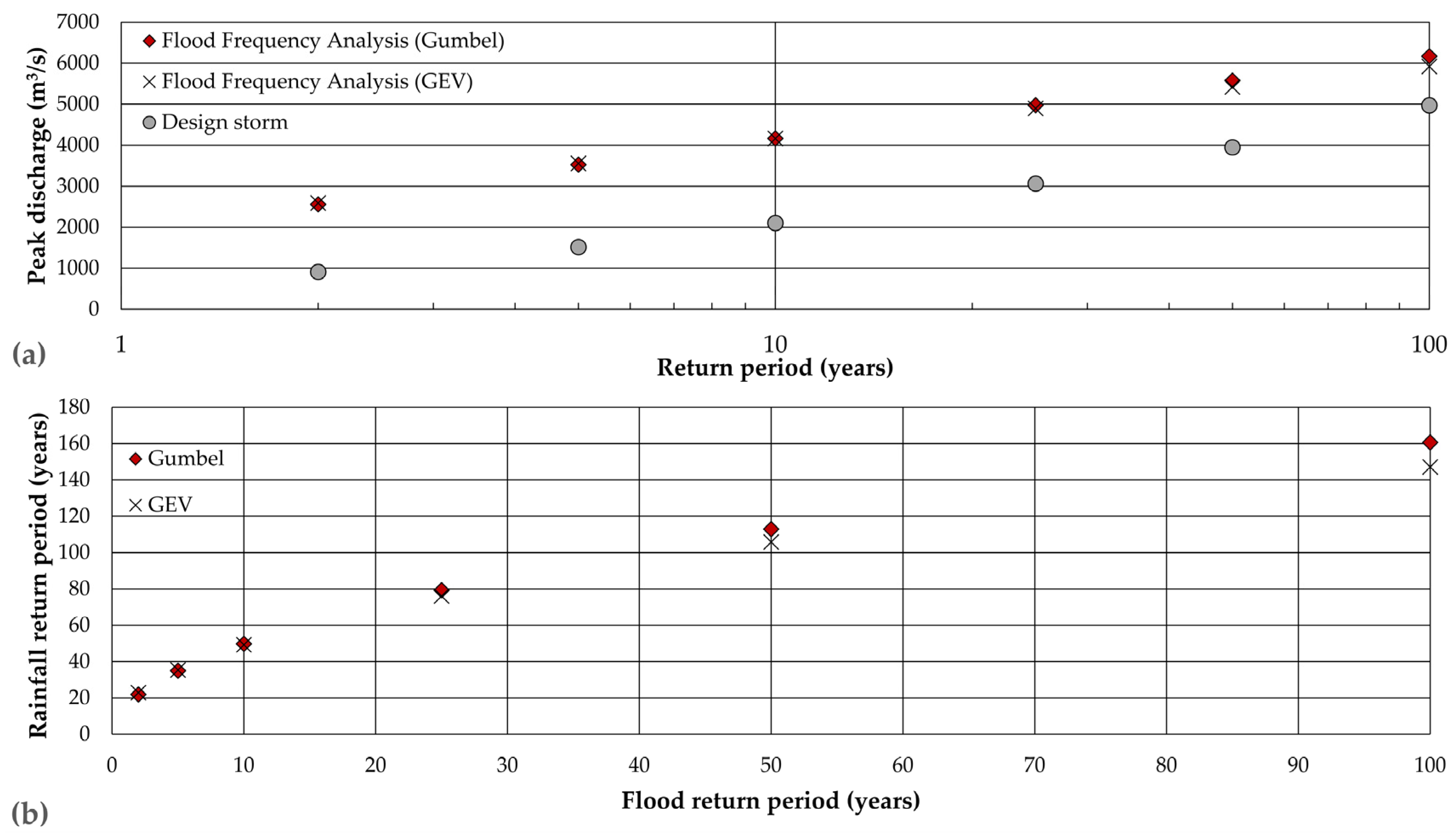
Our results suggested that a flood with a return period of 10 years corresponds to a rainfall with a return period of about 25 years and a flood with a 50-year return period corresponds to rainfall with a return period of about 110 years (
Figure 6b). According to Sutcliffe [
9], a flood with a 10-year return period corresponds to a rainfall with a return period of about 50 years and a flood with a return period of 50 years corresponds to a rainfall with a return period of approximately 110 years. As a result, it can be concluded that in all cases larger return periods of rainfall are needed for the design of hydraulic structures in the study area.
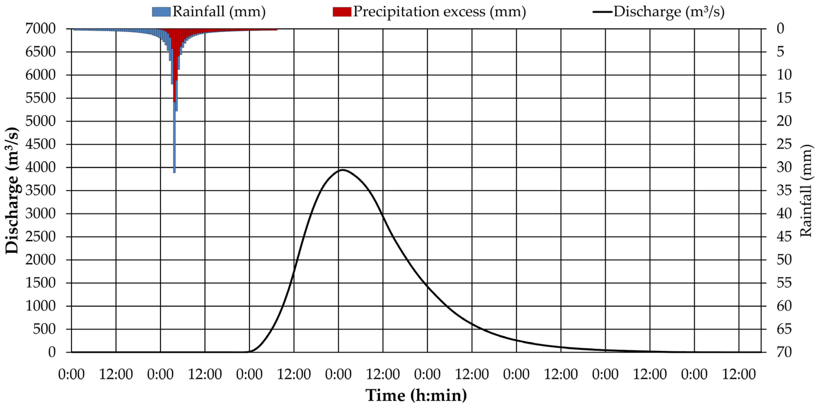
If we had available discharge measurements of an adequate length, we would be able to properly calibrate and validate both models (event-based model and continuous simulation model). However, we believe that our results would not differentiate much and probably the same conclusions could be drawn (i.e., flood return period calculated from the event-based rainfall–runoff model differs from the flood return period calculated based on the results of the continuous rainfall–runoff simulation model). The main reason is associated with the event-based approach. This approach is interrelated with many uncertainties and assumptions (fixed rainfall duration, pre-defined rainfall pattern, pre-determined initial conditions of the catchment, etc.). On the other hand, with the continuous simulation approach, the uncertainty is still present as a result of the simplifications of the real world, but to a lesser extent compared to the event-based approach. In order to account for the inherent uncertainty associated with the design storm approach, the use of different rainfall distribution approaches (e.g., Alternating Block Method, Chicago Design Storm approach, etc.) along with the uncertainty analysis of the model input parameters and the structural uncertainty of the models is proposed.
A different approach than the areal precipitation factor could be examined accounting for the non-uniformity of rainfall excess. In addition, areal factors generally can reduce precipitation depth compared to other approaches. However, since the goal of our study is not to conduct a detailed flood study, the rainfall input to the model is irrelevant. Overall, our research demonstrated that the return periods of rainfall and floods are not equivalent. Their relationship depends on various factors, such as climatological characteristics of the study site, rainfall spatial distribution, antecedent soil moisture conditions, storage capacity of the soil and climate modes, among others.
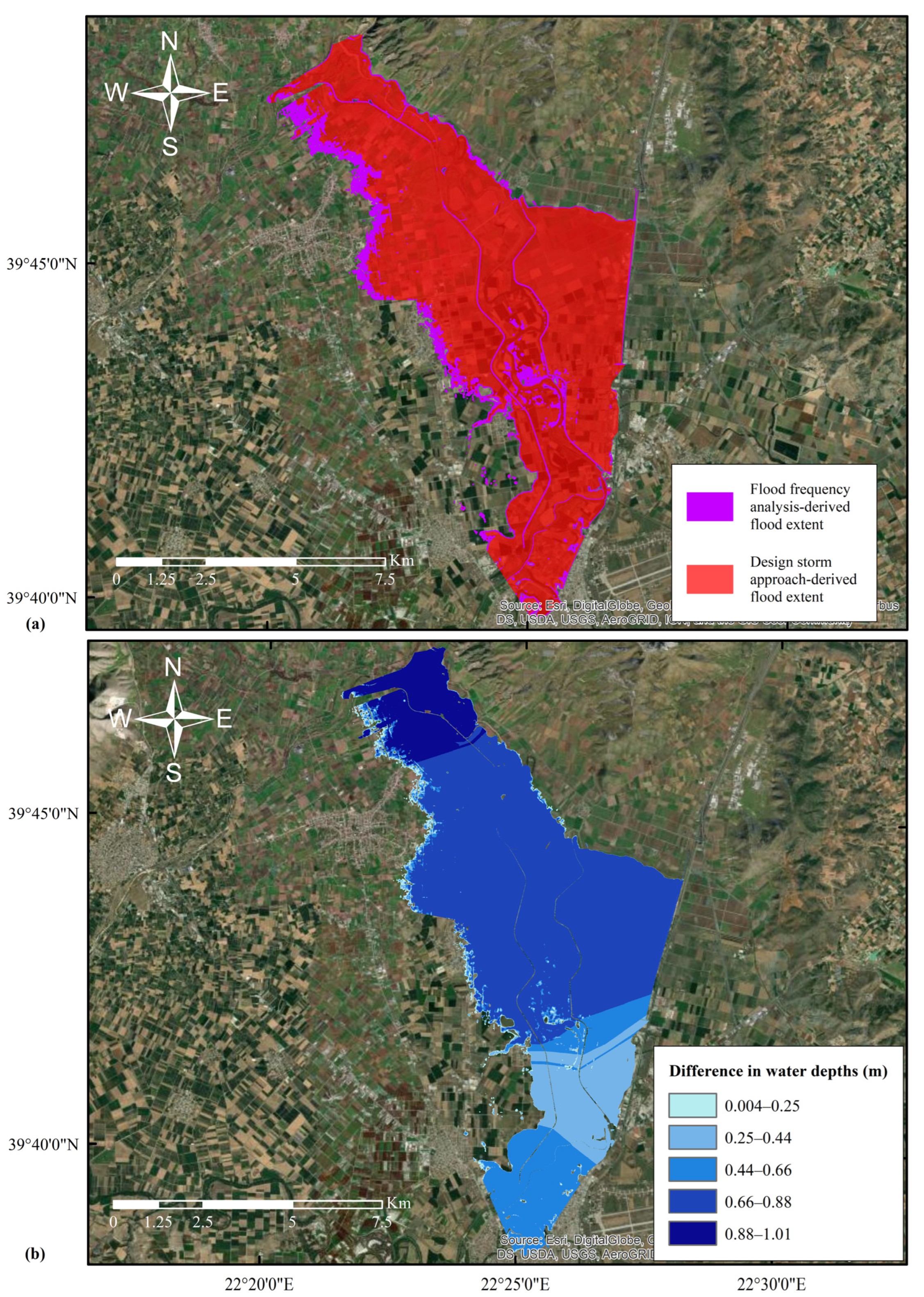
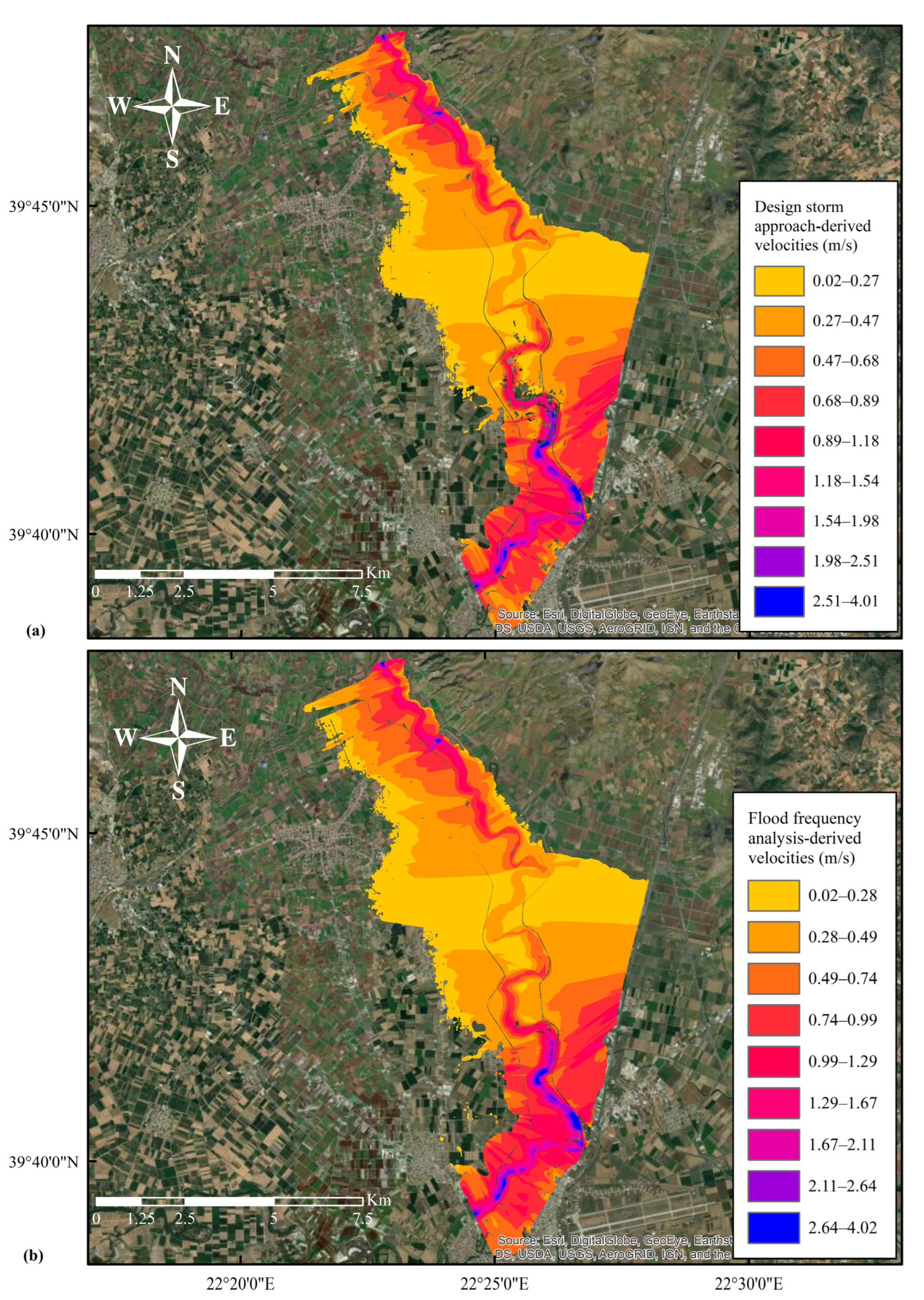
It can be concluded that rainfall return period is the same with the flood return period only under certain circumstances and only for very low probabilities of occurrence. For this reason, it is proposed that flood quantiles and flood hazard assessment should be estimated based on flood frequency analysis, either by means of observed flows or by means of synthetic flows developed by continuous simulation and not by using the design storm approach. However, as already stated, this is not always possible especially in data-scarce areas. Thus, the use of continuous simulation is proposed, in conjunction with re-analysis and/or satellite rainfall data sets. In addition, this study successfully demonstrated that the flood hazard estimated employing the design storm approach is significantly lower than the flood hazard estimated by the continuous simulation and flood frequency analysis approach. For example, the design storm approach underestimated flow velocities by up to 0.5 m/s and inundation depths by up to 1 m, which may be extremely crucial when estimating the subsequent flood damage. The main reason for those differences is associated with the difference between the return period of rainfall and the return period of floods as already discussed.
It must be stated that the hydrodynamic simulation was only performed for the 50-year return period, for both approaches (i.e., design storm and continuous simulation and flood frequency analysis). In addition, our sample data was rather limited to 22 years of rainfall. As a result, extrapolation to low probabilities of occurrence (high return periods) may result in large uncertainties and is not recommended.
The application of the same methodological framework in a different basin, in which high resolution rainfall–runoff measurements of sufficient length (>50 years) are available, is envisaged in the future. The same framework could also be used employing regional frequency analysis. Furthermore, different theoretical distributions could be assessed (e.g., Log-Pearson type III, Wakeby, etc.) and incorporated in the assessment exercise. In addition, the same approach should be applied in different basins with different topographical, physiographical and climatological characteristics. Moreover, the proposed assessment framework could be expanded to include in the analysis, the rainfall duration, the rainfall temporal distributions, the antecedent moisture conditions, etc. Finally, the uncertainty stemming from various sources (e.g., uncertainty of rainfall–runoff measurements, structural uncertainty of the models, parametric uncertainty, etc.) should be studied and quantified.
5. Summary and Conclusions
The prevailing approach (i.e., design storm approach) for the design of hydraulic structures is applied and compared with the continuous simulation and flood frequency analysis approach. The aim is to test the hypothesis if the rainfall return period is equivalent to the flood return period. Initially, rainfall frequency analysis for the design storm approach was undertaken. Then, the results of rainfall frequency analysis were used as an input to a hydrologic model (HEC-HMS; event-based simulation) and the estimated peak, for a given return period, was used as an input to a hydrodynamic model (HEC-RAS). On the other hand, rainfall was used an input to a hydrologic model (HEC-HMS; continuous simulation). Afterwards, the annual maxima series were extracted and flood frequency analysis was undertaken employing two widely used extreme value distributions (i.e., Gumbel and GEV). The estimated quantile (flood peak), for a given return period, was used as an input to a hydrodynamic model for estimating inundation depth, flow velocities and flood extent. Finally, the results of the two aforementioned approaches were compared in terms of estimated quantiles, inundation depths, flow velocities and flood extent.
The results revealed that, in all cases, the design storm approach significantly underestimated flood peaks and as a consequence, the inundation depths, flow velocities and flood extent were also underestimated. This is a crucial finding that shall be taken under consideration by practitioners and engineers working in the water related industry. A generalized relationship and the factors that are incorporated (e.g., size or morphology of the basin) between these two return periods is an open future challenge that should be addressed by the research community.
The main approach used today for estimating flood hazard is the design storm approach. Intensity–Duration–Frequency curves are developed using observed rainfall depths and then used as an input to a hydrologic model for estimating peak discharges. Finally, estimated discharges are used as an input to a hydraulic model for estimating flood hazard. The main drawback of the design storm approach is that it assumes that rainfall return period is equal to flood return period. Another alternative is the use of flow measurements and flood frequency analysis. In the present work, it is proposed to move from the design storm approach to the continuous simulation and flood frequency analysis approach for ungauged or partially gauged basins using satellite estimated rainfall. In order to successfully apply the continuous simulation and flood frequency analysis approach, the following steps should be followed: (i) acquisition of high resolution (e.g., 5 min or less) rainfall measurements; (ii) development of the hydrologic model; (iii) estimation of flood peaks; (iv) flood frequency analysis and estimation of return periods of flood events; and (v) development of the hydraulic model and estimation of flood hazard maps for different return periods. It must be mentioned that in cases where flow measurements are available, they can be used in calibrating/validating both models (hydrologic and hydraulic model). Overall, it can be concluded that the continuous simulation approach is more physically realistic as it does not entail as many assumptions and simplifications of the real world as the event-based approach.
The introduction of new or updated approaches in the design procedures is considered essential. Moreover, especially for data-scarce areas, new and/or emerging technologies such as reanalysis datasets, satellite datasets and/or radar measurements could be used.

 ,
, 


