Article

Relationship of Rainfall and Flood Return Periods through Hydrologic and Hydraulic Modeling

by
Harris Vangelis
1,
Ioanna Zotou
1,
Ioannis M. Kourtis
1,
Vasilis Bellos
2 and
Vassilios A. Tsihrintzis
1,*
1
Centre for the Assessment of Natural Hazards and Proactive Planning & Laboratory of Reclamation Works and Water Resources Management, School of Rural, Surveying and Geoinformatics Engineering, National Technical University of Athens, 9 Heroon Polytechniou St., Zographou, 15780 Athens, Greece
2
Laboratory of Ecological Engineering and Technology, Department of Environmental Engineering, Democritus University of Thrace, 67100 Xanthi, Greece
*
Author to whom correspondence should be addressed.
Water 2022, 14(22), 3618; https://doi.org/10.3390/w14223618
Submission received: 22 August 2022 / Revised: 5 November 2022 / Accepted: 7 November 2022 / Published: 10 November 2022

Abstract

:
In order to examine the relationship between rainfall return periods and flood return periods, the design storm approach is compared to the rainfall–runoff continuous simulation and flood frequency analysis approach. The former was based on rainfall frequency analysis and event-based hydrological simulations, while the latter was based on continuous hydrological simulations and flood frequency analysis. All hydrological simulations were undertaken employing the HEC-HMS software. For the rainfall frequency analysis, the Generalized Extreme Value (GEV) probability distribution was used. For the flood frequency analysis, both the Extreme Value Type I (Gumbel) and GEV theoretical distributions were used and compared to each other. Flood hazard (inundation depth, flow velocities and flood extent) was estimated based on hydrodynamic simulations employing the HEC-RAS software. The study area was the Pineios catchment, upstream of Larissa city, Greece. The results revealed that the assumption of equivalent return periods of rainfall and discharge is not valid for the study area. For instance, a 50-year return period flood corresponds to a rainfall return period of about 110 years. Even if flow measurements are not available, continuous simulation based on re-analysis datasets and flood frequency analysis may be alternatively used.

1. Introduction

Flood discharge probabilities and their relationship with extreme rainfall probabilities is not a well-addressed subject in the literature; hence, it is a very interesting subject from both theoretical and practical perspectives. Flood design is based on extreme value analysis of observed flood peak discharges at a site. However, the measurements of flood discharges are not often available, at least not in time series of adequate lengths. For this reason, hydrologists tend to estimate design floods based on design storms [1,2]. Observed rainfall is used for extracting extreme values (i.e., annual maxima series approach, peak over threshold method), estimating the design rainfall of a given return period, and then, the estimated rainfall is used as an input for a rainfall–runoff model. The aforementioned approach, called the design storm method, is widely applied and has prevailed in engineering practice (e.g., [3]), especially in urban areas where runoff data are very rarely available. The assumption of equivalent (i.e., equal) return periods of rainfall and flood flow may hold true in the case of a block rainfall with fixed duration, invariant rainfall, invariant routing, invariant discharge and a runoff coefficient that remains constant over the rainfall duration. However, in real world basins this is not the case, and the return period of rainfall is not the same as the return period of peak discharge. As a result, researchers have raised concerns regarding the design storm method (e.g., [4,5]).
Pilgrim and Cordery [6] addressed the problem, employing the rational method, by providing runoff coefficients for which the return periods of the design storm will produce flood peaks with the same return periods as the observed ones. Alfieri et al. [7] provided correction factor(s) for the accurate estimation of design floods. Viglione and Blöschl [8] stated that the relation between the storm return period and flood return period is not well understood. They concluded that for storms with varying duration, the return period of floods is always greater than that of the rainfall. Breinl et al. [5] examined the relationship between flood and rainfall return periods and proposed a novel framework for comparing (elasticity of floods to rainfall extremes) annual maxima rainfall (in the form of intensity–duration–frequency curves) with annual maximum streamflow. The proposed approach was applied in 314 rain gauges and 428 streams in Austria. Sutcliffe [9] reported that storms with return periods of 2, 8, 17, 35, 50, 81, 140, 300, 520 and 1000 years correspond to flood flows with return periods of 2.33, 5, 10, 20, 30, 50, 100, 250, 500 and 1000 years, respectively.
The Extreme Value Theory was introduced by Gumbel [10] and mainly involves the following steps: (i) observed flood data ordering; (ii) fitting of a theoretical distribution function and parameter estimation; and (iii) extrapolation of the tails of the distribution to large return periods (low probabilities of occurrence). Various researchers have applied extreme value analysis to estimate the probabilities of extreme flood events, rainfall events, sea levels etc. (e.g., [11,12,13,14,15,16,17,18,19]). A wide variety of theoretical distributions have been used for rainfall and flood frequency analysis (e.g., [20]). The most widely used distributions are: Normal (e.g., [21]), Log-normal (e.g., [22]), Log-normal with three parameters (e.g., [23]), Exponential (e.g., [24]), Two-component exponential (e.g., [25]); Gamma (e.g., [8]), Pearson Type III (e.g., [26]), Log-Pearson Type III (e.g., [27]), Extreme Value Type I (Gumbel; e.g., [28]), Extreme Value Type II (Fréchet; e.g., [29]), Extreme Value Type III (Weibull; e.g., [30]), Generalized Extreme Value (GEV; e.g., [31]), Generalized Pareto (e.g., [32]), Generalized logistic (e.g., [33]) and Wakeby (e.g., [23]). Countries have adopted different theoretical distributions as standard models for flood and/or rainfall frequency analysis [20]. For example, in the United States of America and Australia, the Log-Pearson Type III is the standard model for flood frequency analysis, while in the United Kingdom, the Generalized logistic is the standard model for extreme value analysis of floods. In Greece, the GEV theoretical distribution is the standard model for rainfall frequency analysis. For a review of recent applications of frequency analysis in the field of hydrology, the interested reader is referred to WMO [20], Grimaldi et al. [34] and Madsen et al. [35].
Different approaches have been presented in the literature for the estimation of the parameters of a theoretical distribution. The most widely used approaches are [34]: the method of moments, the method of maximum likelihood and the L-moments approach. The method of L-moments constitutes a combination of the Probability weighted moments and was standardized by Hosking [36]. In the present work, the GEV distribution was selected for rainfall extreme value analysis with parameters estimated employing the L-Moments method, as this is the proposed method by the technical specifications in Greece. For the flood frequency analysis, two distributions were examined, namely the Extreme Value Type I (Gumbel) and the GEV with parameters estimated using the L-Moments method [37]. The L-Moments method was preferred as it is rather simple, it characterizes efficiently the sampled data and it is not affected by the variability of the sampling approach [36].
The aim of this study was to first apply the two above-described approaches (i.e., the design storm approach, and continuous simulation and flood frequency analysis) using satellite rainfall data; then, to relate the rainfall return periods with flood return periods derived using hydrologic/hydraulic modeling; and finally, compare the results. Comparison was performed in terms of peak discharge at the outlet of the studied basin (i.e., design storm results vs. continuous simulation and flood frequency analysis results) and in terms of flood hazard (i.e., flood extent, inundation depths and flow velocities). Flood hazard was estimated based on the results of the hydrodynamic model. To the best of our knowledge, this is one of the very few attempts (e.g., [9]) trying to relate rainfall and flood return periods.

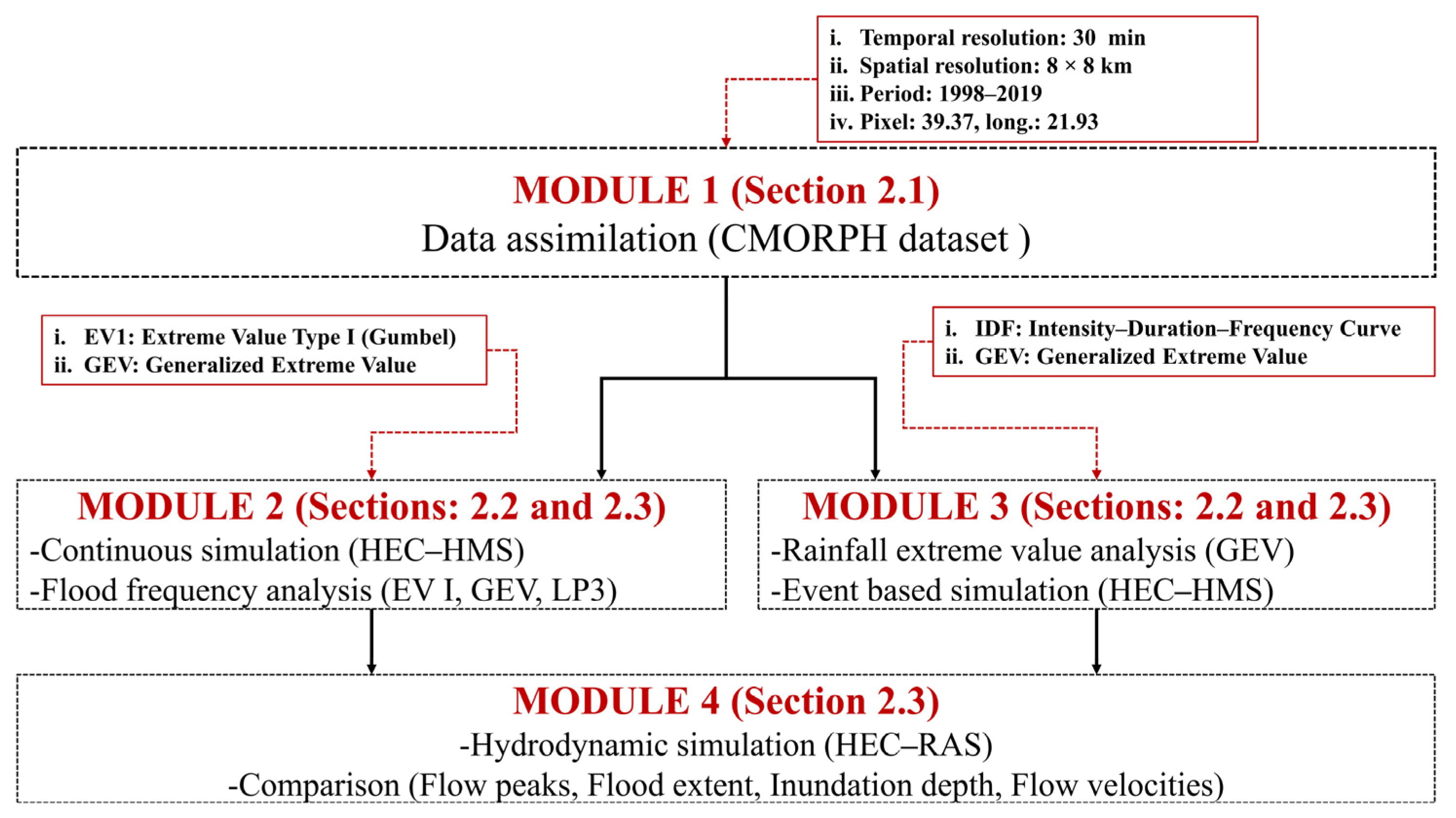
2. Materials and Methods

The proposed methodological approach is presented in Figure 1 and fully described in Section 2.1, Section 2.2 and Section 2.3. It consists of four modules. The first module is associated with the acquisition of data (digital elevation model, rainfall satellite data land uses, etc.). The second module includes continuous simulation employing the widely used hydrological model HEC-HMS [38] and frequency analysis of the synthetic peak discharges. Frequency analysis was based on one event per hydrological year (1 October to 30 September; Annual Maxima Series approach). The third module is associated with the use of rainfall satellite data and the development of Intensity–Duration–Frequency (IDF) curves employing the Generalized Extreme Value Distribution (GEV) and the hydrologic simulation (event-based simulation) of the basin. Finally, the fourth and final module of the proposed framework involves hydrodynamic simulation using HEC-RAS software (e.g., [38]) based on the two aforementioned approaches and the comparison of the results.

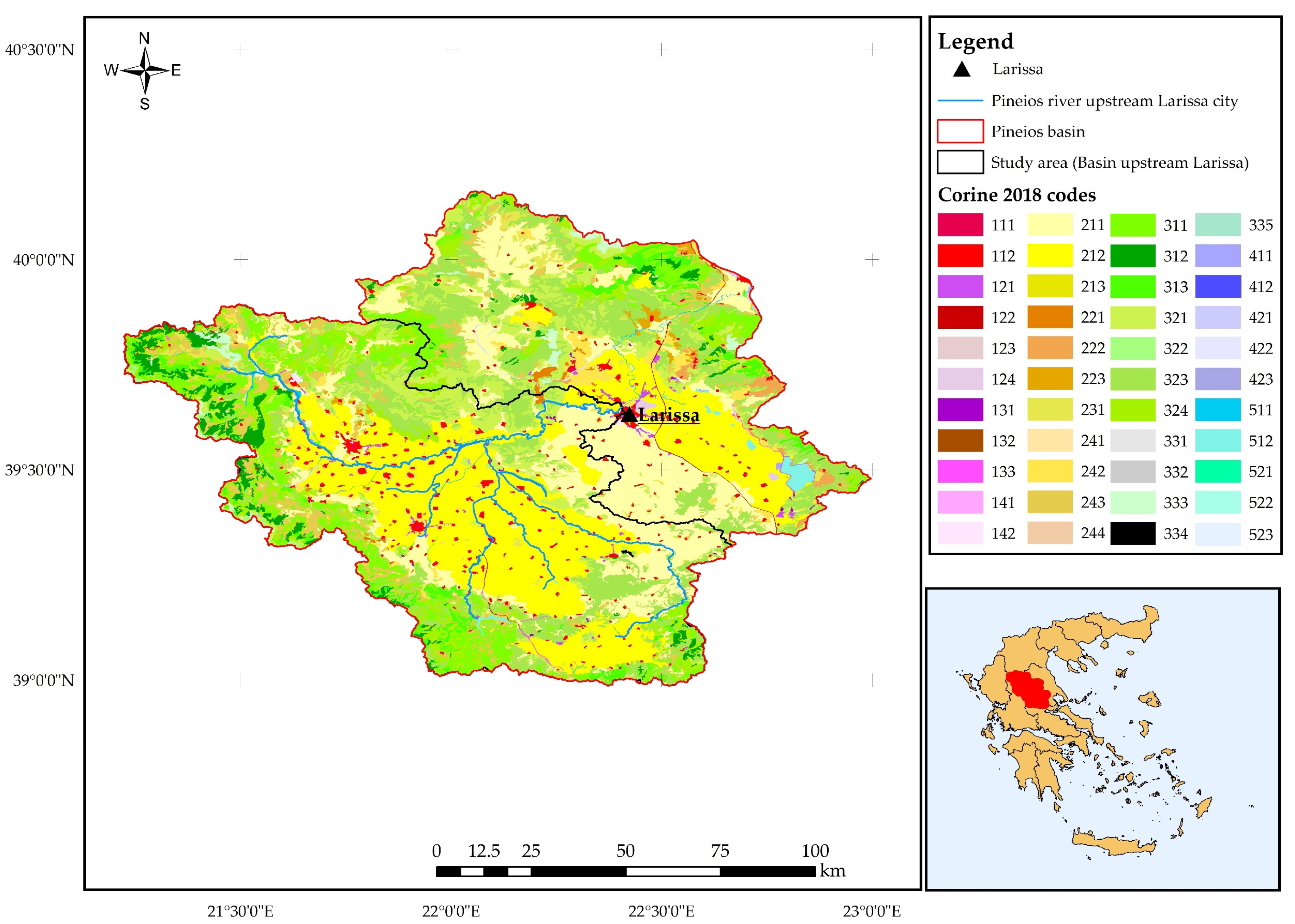
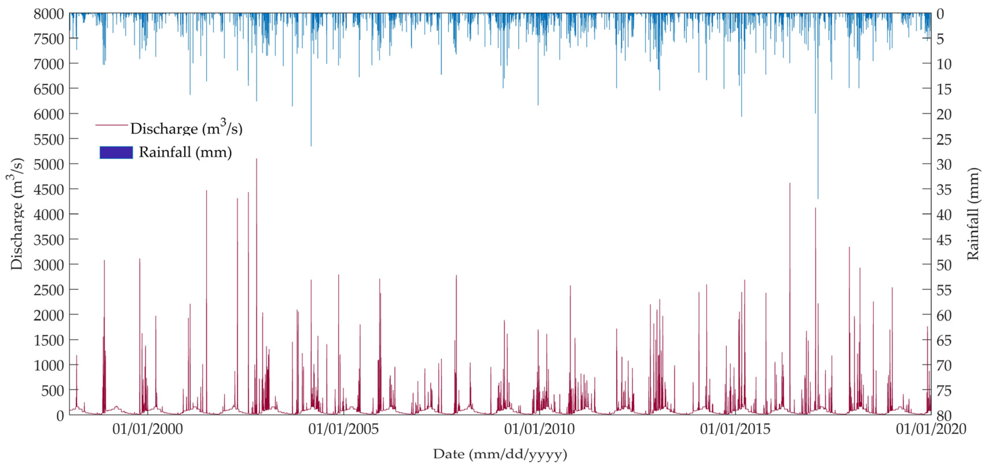
2.1. Study Area and Data

The above-described methodology was applied in part of Pineios River basin. The Pineios River is the third longest river in Greece; it discharges into the Aegean Sea after it crosses the eastern part of central Greece. The basin covers an area of about 11,000 km2 with a length of about 260 km. The wet period is from November to February with the rainiest months being November to December. On the other hand, during the summer months (June to August), the rainfall is almost zero. The mean annual flow for the Pineios River basin is estimated at about 3500 × 106 m3. According to Bathrellos et al. [39], the regime of the Pineios River flow, for the main tributary, can be characterized as perennial, with large differences between winter and summer. For instance, near its delta, the mean average discharge ranges from more than 150 m3/s in February and March to about 10 m3/s in August and September [39].
The study area is the Pineios catchment, upstream of Larissa city in Greece (Figure 2). It covers an area of approximately 6508 km2 [38]. The altitude ranges from 67 m a.s.l. to about 2700 m a.s.l. with the mean altitude estimated at about 421 m a.s.l. Figure 2 also presents the land uses in the study area, according to 2018 Corine Land Cover. These data were used for estimating different parameters (e.g., CN parameter) needed for the hydrologic simulation. The land use/land cover types are presented in detail in Table 1, i.e., Corine code, description and percent of the total study area covered per land use/land cover type.
The CMORPH rainfall reanalysis dataset [40] was utilized, as it has the highest spatial (8 km × 8 km) and temporal resolution (30 min) and the longest available record (1 January 1998–31 December 2019). Data were downloaded from the data server of the Climate Prediction Center (CPC) of the National Oceanic and Atmospheric Administration (NOAA; [41]) for the pixel closest to Karditsa station (lat.: 39.37, long.: 21.93, altitude: 103 m a.s.l.). The GEV distribution was used for modeling the rainfall annual maxima series. The parameters of GEV distribution were estimated based on the method of L-Moments [37]. Parameter estimation was undertaken for time scales ranging from 30 min to 48 h and for return periods ranging from 10 to 100 years. The Hydrognomon software was used for all the computations [42]. Table 2 presents the sample statistics for several time scales. The maximum rainfall depth for the different time scales ranges from 37 mm to 140 mm, while the minimum rainfall depth ranges from about 7 mm to about 38 mm. The coefficient of skewness was found to be positive for all time scales indicating tail on the right (positive skewed) and also that the data are not normally distributed. Moreover, it can be observed that for all time scales examined, the mean is greater than the median. As a result, it can be concluded that the empirical distribution is positively skewed.
It must be stated that we have chosen to apply this procedure in order to better understand the differences of the two approaches, assuming that:
  • Satellite rainfall is free of biases;
  • The rainfall distribution is produced based on the empirical Alternating Block Method [1] assuming specific time step and storm duration;
  • The rainfall losses are estimated using the SCS Curve Number (CN, land uses and soil in the study area);
  • Continuous simulation and flood flow frequency analysis was conducted using the peak discharges generated by the hydrological model;
  • One flood per hydrological year is selected so that the events are identically distributed and statistically independent.

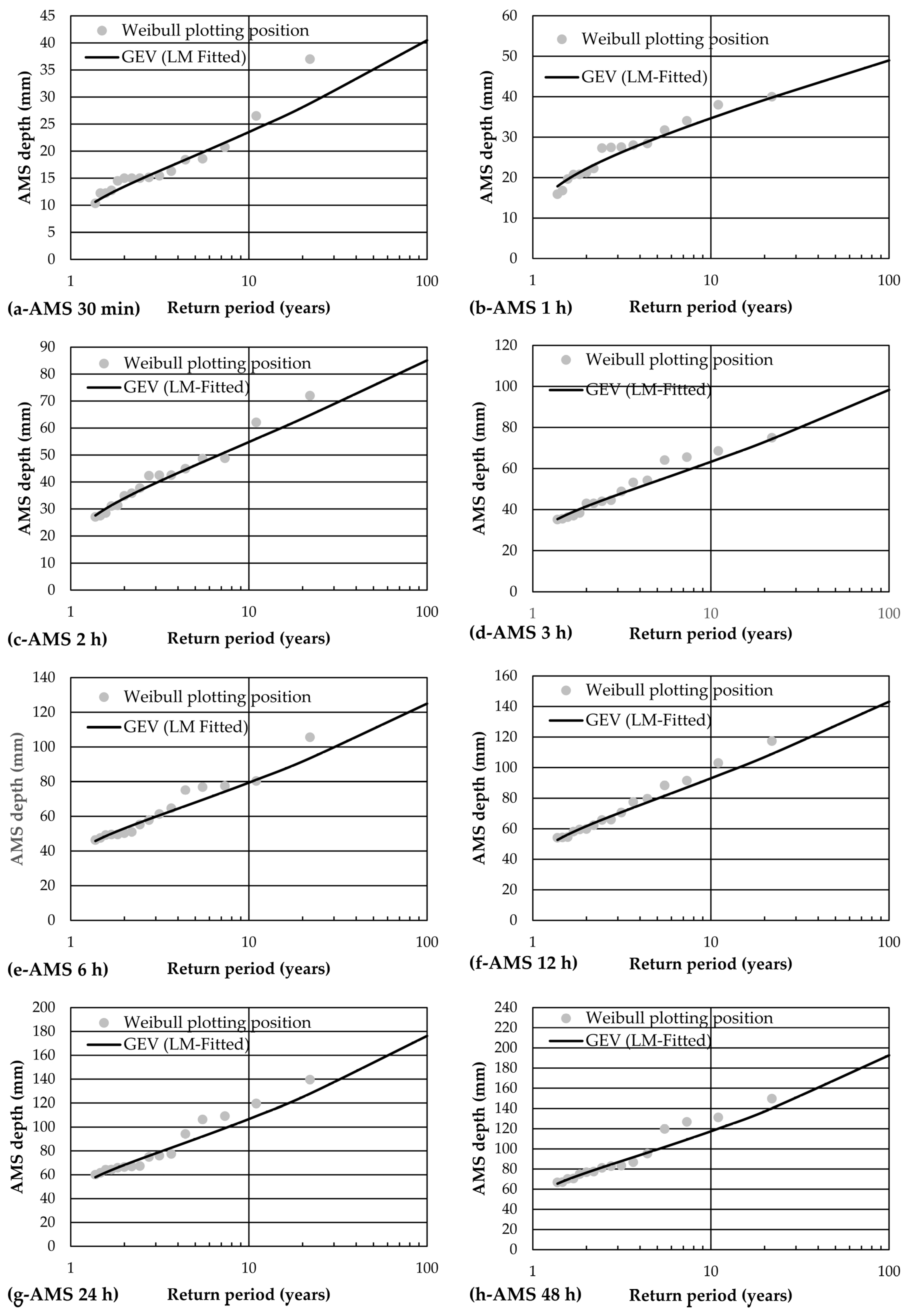
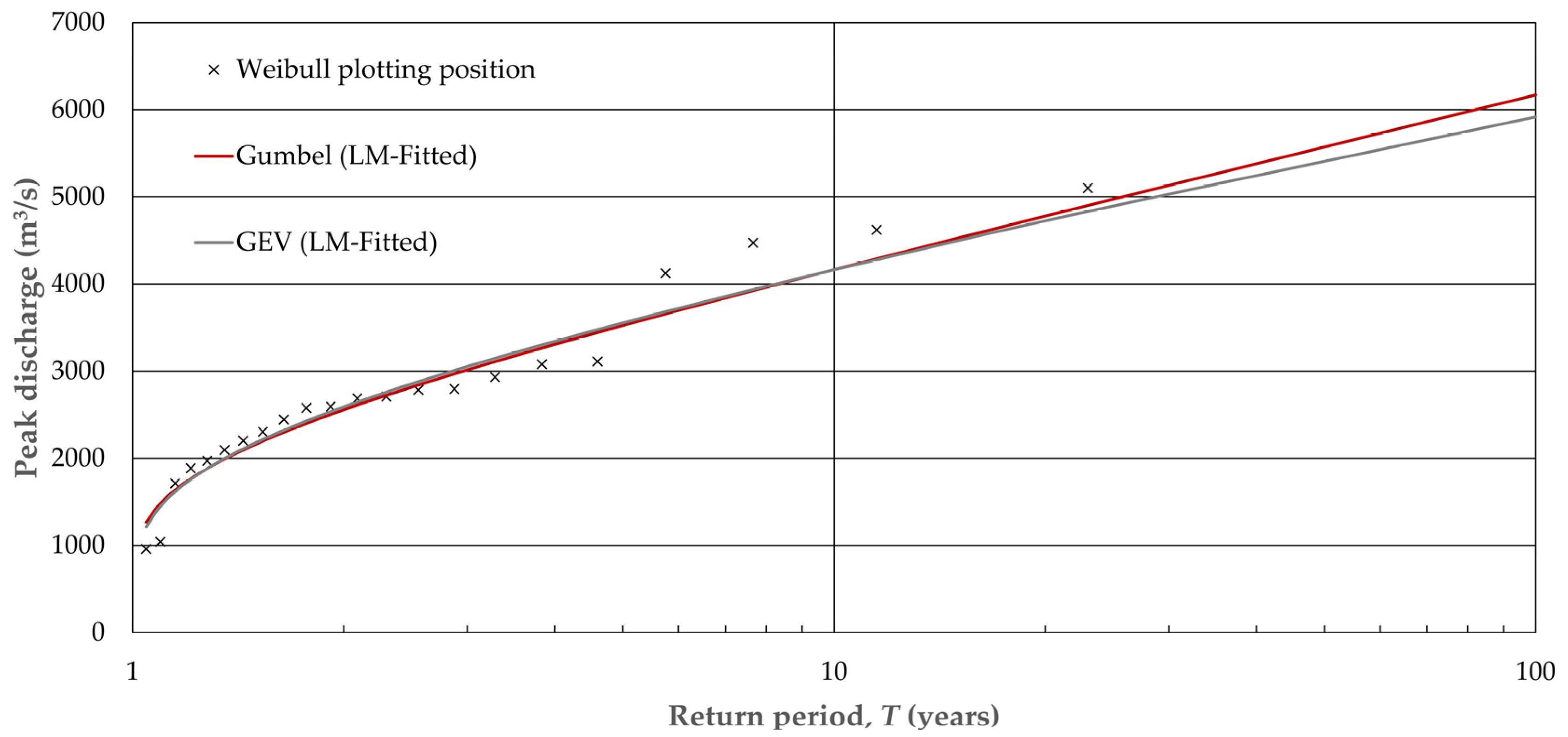
2.2. Extreme Value Analysis

The GEV distribution combines the three asymptotic extreme value distributions into a single distribution. The shape parameter (κ) determines the type of extreme value distribution. If κ is greater than zero, the Extreme Value Type III (Weibull) is indicated, if κ is lower than zero the Extreme Value Type II (Fréchet) is indicated, and if κ is zero the Extreme Value Type I (Gumbel) is indicated. The cumulative distribution function of GEV is:
F ( x ) = exp { [ 1 k α ( x μ ) ] 1 k }   f o r   k 0
F ( x ) = exp { exp [ 1 α ( x μ ) ] } }   f o r   k = 0
where: μ is the location parameter, α is the scale parameter and k is the shape parameter of the GEV distribution.
The inverse of Equations (1) and (2), quantile functions, are:
x ( T ) = μ + α { 1 ( logF ) } k / k ,     f o r   k   0
x ( T ) = μ α log ( log F ) ,       f o r   k = 0
where all the parameters have been already defined.
The cumulative distribution function of Gumbel distribution is:
F ( x ) = exp { exp [ 1 α ( x μ ) ] }  
where all the parameters have been already defined.
The quantile function, inverse of Equation (5), for Gumbel distribution is:
x ( T ) = μ α log ( F )
where all the parameters have been already defined. The parameters of both probability distributions were estimated based on the method of L-Moments [37].
Finally, generalized Intensity–Duration–Frequency (IDF) curves were developed, for the Karditsa pixel (extracted from the CMORPH rainfall satellite data), based on the approach proposed by Koutsoyiannis et al. [43]:
i = α ( T k μ ) ( 1 + t / θ ) η
where: i is rainfall intensity (mm/h), α′ = α/k, μ′ = 1 − , t is rainfall duration (h), θ and η are coefficients and all other parameters have been already defined.
The point rainfall derived from the IDF curve was transformed to the catchment IDF curve by employing the areal reduction factor (r) proposed by Leclerc and Schaake [44]:
r = 1 exp ( 1.1 t 1 / 4 ) + exp ( 1.1 t 1 / 4 0.004 A )
where: r is the areal reduction factor, t is rainfall duration (h) and A is the catchment area (km2). Point rainfall depth was transformed to areal rainfall depth by multiplying it with the aforementioned coefficient.

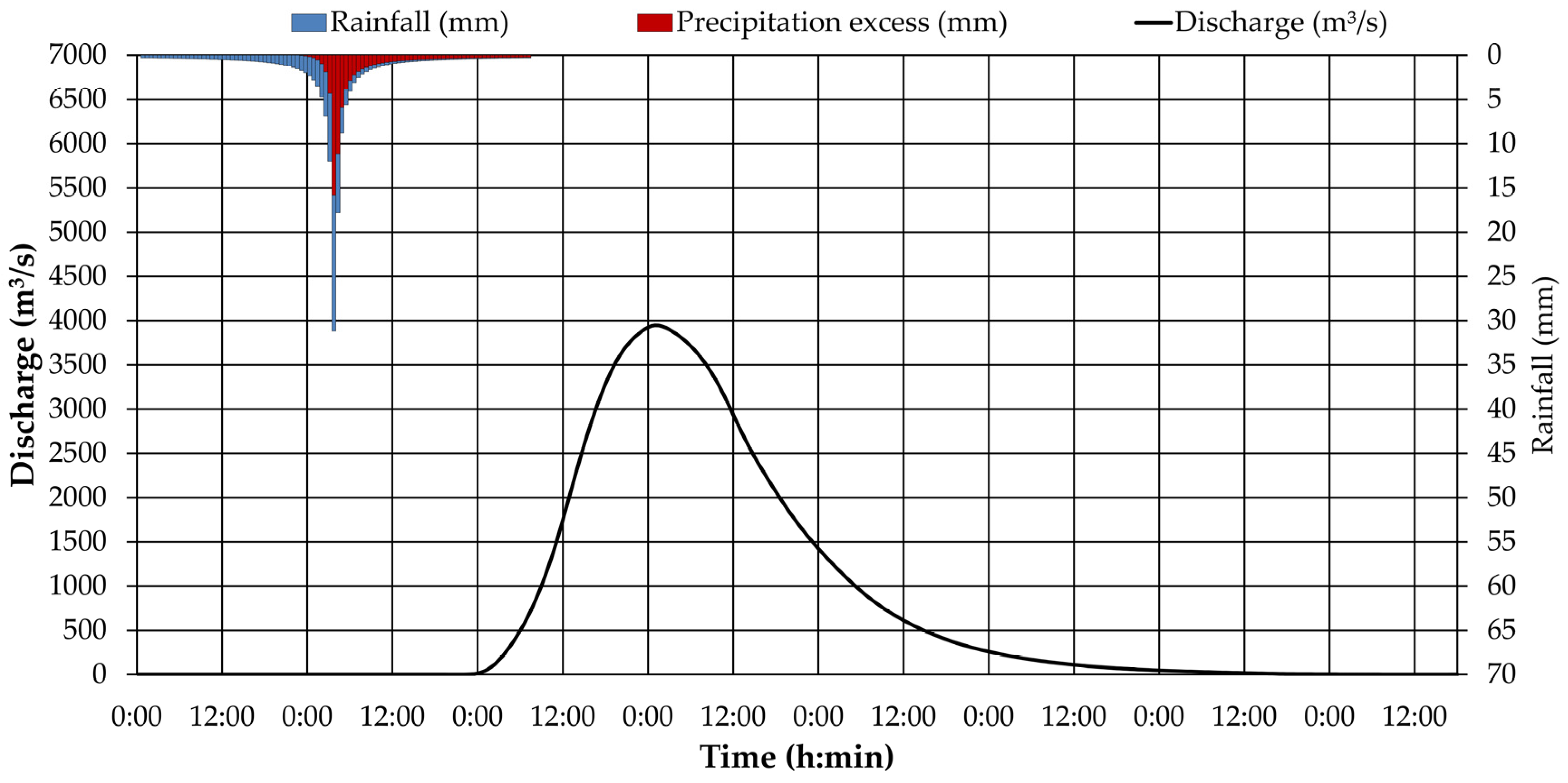
2.3. Hydrologic-Hydrodynamic Modeling

The basin was not divided into sub-catchments for neither the event-based nor the continuous simulation schemes. We chose to not delineate our catchment as our goal was to relate the rainfall return periods with flood return periods and compare the derived results. In addition, flow measurements were not available in our study area, and as a result, we decided not to delineate our catchment in sub-basins in order to not introduce uncertainty related to the estimation of routing (hydrologic or hydraulic) parameters. For the event-based simulation, the Soil Conservation Service (SCS) Curve Number (CN) approach was used to model the losses. Based on the land use/land cover data from 2018 Corine Land Cover and the soil data for the study area, the area weighted average CN was estimated at about 68. In addition, the Unitless SCS Unit Hydrograph was selected as the transform method. The time of concentration was estimated, employing the Giandotti empirical Equation [2,45], equal to 37.6 h.
For the continuous simulation, the following methods were employed: (a) the Simple Canopy method [46], to represent the precipitation intercepted by the plant canopy and used for evapotranspiration; (b) the Deficit and Constant loss method [46] in order to describe infiltration processes in the soil layer; (c) the SCS Unit Hydrograph transform method [1,2,46]; and (d) the constant monthly Baseflow method [46]. The Deficit and Constant loss method describes the changes in soil moisture content through a single soil layer and is suitable for continuous simulation. It employs four parameters, i.e., the initial and maximum deficits (mm), the constant rate (mm/h) and the percent of impervious area (%). The initial deficit parameter denotes the initial condition of the soil layer at the beginning of the simulation, in terms of the storage capacity that is not filled, and thus, is available for receiving precipitation either directly or indirectly through the canopy. Respectively, the maximum deficit stands for the maximum water capacity of the soil. The constant rate represents the infiltration/percolation rates after the soil layer reaches its maximum capacity and can be approximated with the saturated hydraulic conductivity [46]. The Deficit and Constant loss method should be combined with a Canopy method to simulate the interaction between canopy and soil layers. The plant canopy intercepts precipitation, as long as its maximum storage capacity is not exceeded, thus decreasing the total amount of rainfall reaching the soil layer. In addition, by means of the canopy layer, water is extracted from the soil through the plants according to their evapotranspiration demands. We decided to represent infiltration through the Deficit and Constant loss method, since it is suitable for performing continuous simulation, and also, consists of only one soil layer and, hence, has lower requirements in terms of input parameters compared to the rest of the methodologies available in the HEC-HMS software. Similarly, the Simple Canopy method was selected instead of the Dynamic one in an effort to not introduce uncertainty associated with the estimation of the input parameters. Initial values for the Deficit and Constant loss method parameters were estimated as weighted average values based on the predominant soil texture classes throughout the study area. Regarding the baseflow, the constant monthly method was selected, according to which a constant baseflow value is assumed for each month of the year. In this study, mean monthly baseflow data, acquired from Nalbantis and Koutsoyiannis [47], were utilized.
The continuous hydrologic model was plausibly checked based on the runoff coefficient reported by Nalbantis and Koutsoyiannis [47], who, based on rainfall–runoff measurements for 22 years, reported a mean annual runoff coefficient equal to 0.36. We used this reported value to adjust the most sensitive parameters of our model, i.e., the crop coefficient (kc) and the constant rate of the Deficit and Constant loss method, in a manual and empirical way. The parameters used and their range are presented in Table 3. Finally, flood frequency analysis was applied to the annual maxima series, which resulted from the continuous simulation, using Gumbel and GEV theoretical distributions, in order to estimate flood quantiles for various return periods (2 years to 100 years) as previously described.
The 1D steady state routine of the Hydrological Engineering Center-River Analysis System (HEC-RAS) hydraulic software of the United States Army Corps of Engineers was used to route flood peak discharges estimated from both approaches (e.g., [48,49]). Within HEC-RAS, steady flow calculations are based on the solution of the 1D energy equation, whereas the Momentum equation is exploited in cases of rapidly varied flow, e.g., hydraulic jumps and in river junctions [48].
The geometric representation of the simulated river was developed in HEC-RAS Mapper, upon a fine resolution Digital Elevation Model (5 m × 5 m) and consisted of 305 river cross-sections in total with an average distance spacing of approximately 90 m between the riverbank lines and the stream and flow path centerlines, respectively. Manning’s friction coefficient value was set equal to 0.03 for the main channel and 0.04 for the overbank areas [1,2].

3. Results

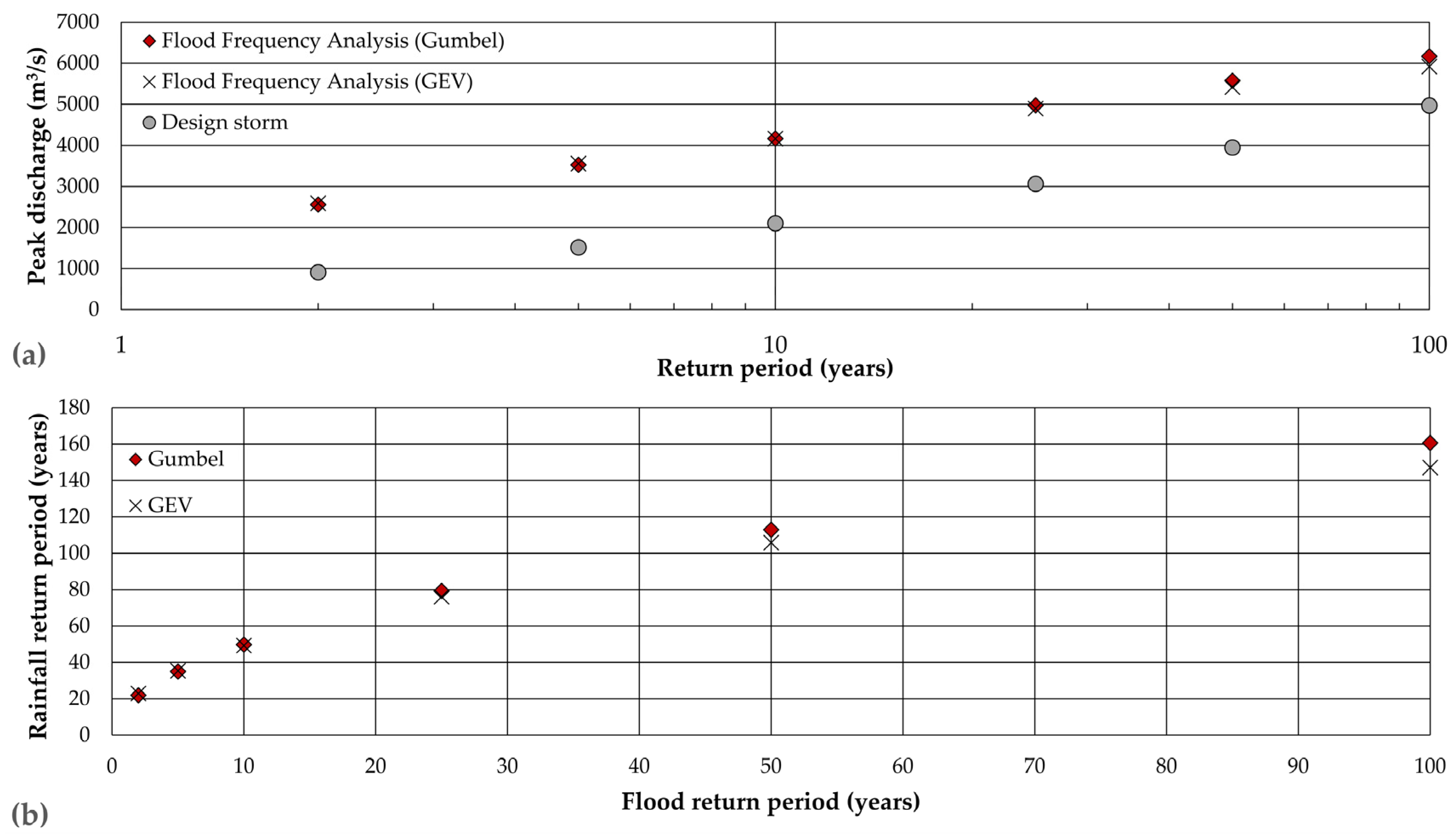
3.1. Design Storm Approach vs. Flood Frequency Analysis

Prior to frequency analysis, the Kolmogorov–Smirnov and chi-squared statistical tests were performed to test the null hypothesis that GEV probability distribution fits the data, for different significance levels (1%, 5% and 10%). In all cases, and for both statistical tests, it was concluded that the null hypothesis cannot be rejected. As a result, GEV distribution can be used to develop IDF curves for the different time scales examined. In addition, a graphical comparison by fitting the theoretical GEV distribution to the sample is depicted in Figure 3. The empirical plotting position was estimated by employing the Weibull unbiased plotting position [50]. The theoretical values using the GEV distribution are presented in Figure 3 as black lines. It can be observed that for low return periods, the GEV distribution describes the annual maxima series of rainfall very well for all the examined time scales (i.e., 30 min to 48 h).
As a result, it was concluded that the GEV distribution was consistent with the data. Equation (9) presents the IDF curve developed from CMORPH data for the pixel representing Karditsa station:
i = 68.73 ( T 0.15 0.45 ) ( 1 + t / 0.996 ) 0.836
where: i is the rainfall intensity (mm/h), t is the rainfall duration (h) and T is the return period (years).
Finally, Table 4 presents the estimated intensity (mm/h) for various rainfall durations (2 to 48 h) and for return periods ranging from 2 to 100 years. These intensities were transformed to areal intensity by applying Equation (8). Since the time of concentration, as mentioned, was estimated at about 37.6 h, the rainfall duration was chosen for the event-based simulation equal to 48 h.
Figure 4 presents the 48 h, 50-year hyetograph indicating that the rainfall used was not constant, and also, the results of the event-based simulation for the rainfall duration of 48 h and return period of 50 years. Peak discharge was estimated at about 4000 m3/s.
The results of the continuous simulation are presented in Figure 5. The simulation was undertaken from 1 January 1998 to 31 December 2019. According to Nalbantis and Koutsoyiannis [47], the mean monthly baseflow ranges from 14.8 m3/s to 156.1 m3/s. The maximum flow was estimated at about 5101 m3/s, while the minimum flow was 959.2 m3/s. The runoff coefficient was calculated equal to 0.36.
Flood frequency analysis was undertaken for the annual maxima series of synthetic peak discharges using Extreme Value Type I (Gumbel) and GEV probability distributions. For assessing the fitting of both probability distributions to the annual maxima series of synthetic peak discharges, the Kolmogorov–Smirnov and chi-squared statistical tests were performed for various significance levels (1%, 5% and 10%). For both distributions and for both statistical tests, it was concluded that both Gumbel and GEV probability distributions can be used for modeling annual maxima flood peaks. Table 5 presents the sample statistics for the annual maxima series of synthetic peak discharges.
Finally, Figure 6 presents the fitting of the theoretical distributions (Gumbel and GEV) to the empirical ones. The Weibull plotting position was used for estimating empirical quantiles. It can be observed that both Gumbel and GEV distributions describe the annual maxima series of synthetic peak discharges at the outlet of the basin very well. Therefore, both distributions are considered appropriate for modeling annual maxima series.
Table 6 and Figure 7 present the comparison between the results derived from the design storm approach and the continuous simulation and flood frequency analysis approach. It can be observed that the design storm approach constantly underestimates the estimated flood quantiles. According to the results, the percent increase for the Gumbel and GEV distributions ranges from about 180% to 25% and from about 185% to 20%, respectively. For instance, for a return period of 2 years, the flood peak estimated based on the results of the continuous simulation and the flood frequency analysis with GEV and Gumbel is 185% and 181%, respectively, greater than the flood peak estimated based on the design storm approach (Table 5 and Figure 6). In addition, it can be observed that flood frequency analysis based on Gumbel and GEV theoretical distributions yields similar results. The percent difference between the two distributions ranges between 1% (for a return period of 2 years) and −4% (for a return period of 100 years). Finally, it can be observed that as the return period increases, the percent difference decreases. This is expected since our sample (rainfall and peak discharges) is only 22 years. As a result, the estimation of large return periods (tails of the distributions) entails a high degree of uncertainty.

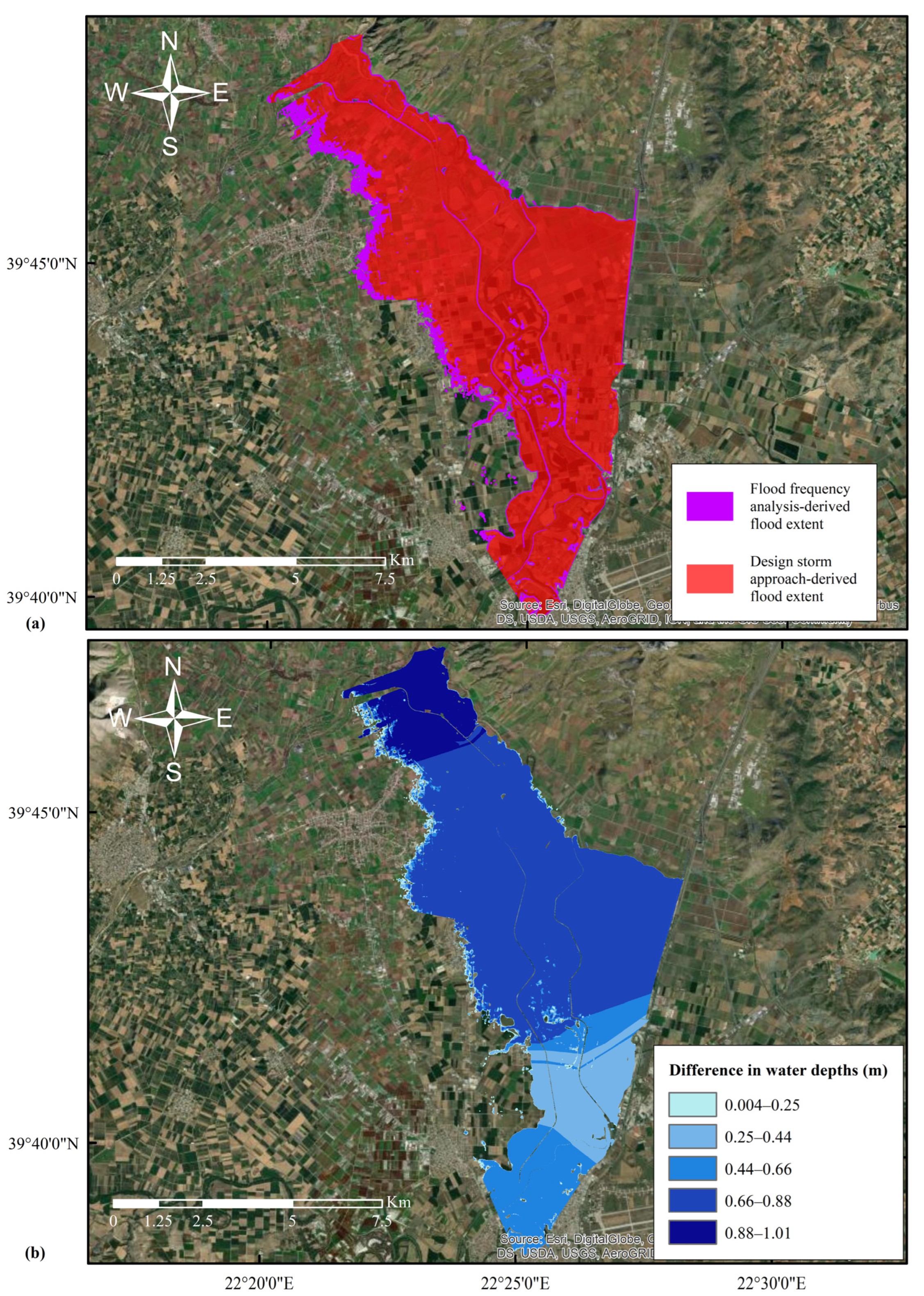
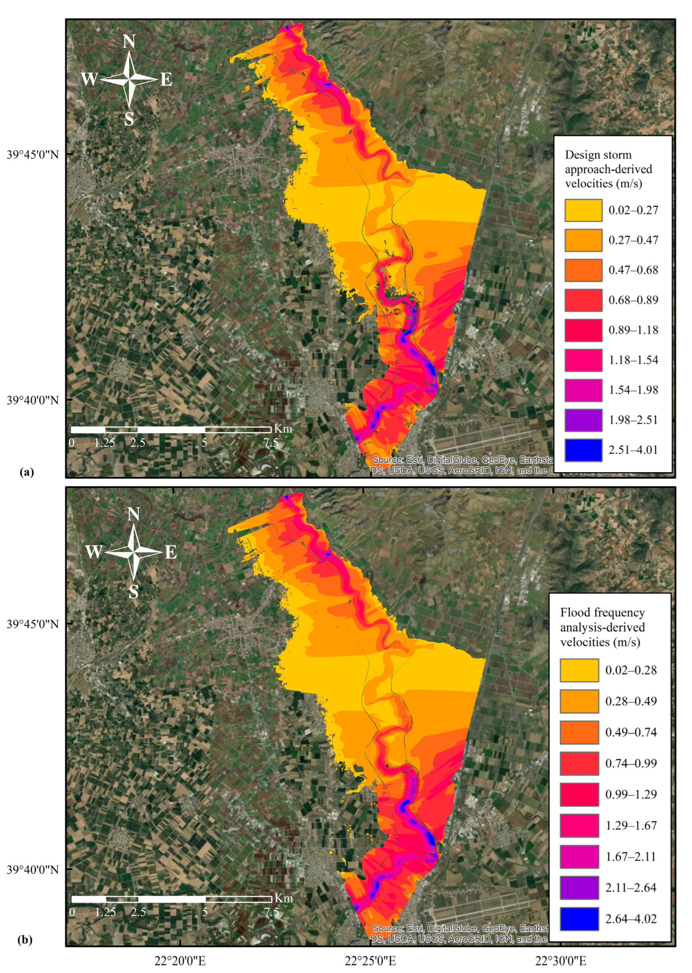
3.2. Hydrodynamic Simulations and Results

Hydrodynamic simulation for both approaches (i.e., design storm approach and continuous simulation and flood frequency analysis approach) was performed employing the HEC-RAS software. It should be noted that the peak discharge derived from the flood frequency analysis using Gumbel probability distribution for a 50-year return period was exploited instead of GEV. The two distributions yielded similar results as previously described, thus, we only exploited Gumbel as the estimated peaks are slightly higher.
Figure 8 presents the derived results with respect to the flood inundation extent (Figure 8a) and the difference between the simulated inundation depths (Figure 8b). As expected, the continuous simulation combined with the flood frequency analysis led to a larger inundated area, compared to the designed storm approach. Specifically, in the former case a flood extent greater by 7.7% was computed, which translates into an approximately 4.4 km2 larger flooded area. Similarly, greater inundation depths emerged from the flood frequency analysis approach, resulting in discrepancies of up to 1 m between the examined scenarios (Figure 8b) for the areas close to the downstream boundary of the model.
Finally, Figure 9a,b present flow velocity distribution throughout the modeled area for both scenarios examined. Again, higher velocities were computed when the continuous simulation with the flood frequency analysis scenario was considered. In particular, according to the derived results, differences in velocities were found to range from 0 to 0.5 m/s for 98% of the modeled area. The results revealed that the proposed methodology is viable and could be applied in other basins and/or even substitute the prevailing approach for designing hydraulic structures (i.e., design storm approach).

4. Discussion

In this work, rainfall frequency analysis for developing Intensity–Duration–Frequency (IDF) curves was applied on the annual maxima rainfall using the GEV distribution, the method of L-moments for distribution fitting and the generalized approach for developing IDF curves proposed by Koutsoyiannis et al. [43]. The time of concentration for the basin is large (37.6 h), but to develop accurate IDF curves, data in sub-hourly time scales are needed. As a result, the CMORPH reanalysis data set was used instead of other reanalysis and/or satellite derived rainfall datasets (e.g., ERA5-Land). In addition, it must be mentioned that a study comparing the various or at least some of the existing global rainfall datasets in terms of rainfall–runoff modeling would be of great interest to the scientific community. Finally, flood frequency analysis for the annual maxima series of synthetic peak discharges (i.e., continuous simulation) took place using Gumbel and GEV probability distributions and the method of L-moments.
Our results suggested that a flood with a return period of 10 years corresponds to a rainfall with a return period of about 25 years and a flood with a 50-year return period corresponds to rainfall with a return period of about 110 years (Figure 6b). According to Sutcliffe [9], a flood with a 10-year return period corresponds to a rainfall with a return period of about 50 years and a flood with a return period of 50 years corresponds to a rainfall with a return period of approximately 110 years. As a result, it can be concluded that in all cases larger return periods of rainfall are needed for the design of hydraulic structures in the study area.
If we had available discharge measurements of an adequate length, we would be able to properly calibrate and validate both models (event-based model and continuous simulation model). However, we believe that our results would not differentiate much and probably the same conclusions could be drawn (i.e., flood return period calculated from the event-based rainfall–runoff model differs from the flood return period calculated based on the results of the continuous rainfall–runoff simulation model). The main reason is associated with the event-based approach. This approach is interrelated with many uncertainties and assumptions (fixed rainfall duration, pre-defined rainfall pattern, pre-determined initial conditions of the catchment, etc.). On the other hand, with the continuous simulation approach, the uncertainty is still present as a result of the simplifications of the real world, but to a lesser extent compared to the event-based approach. In order to account for the inherent uncertainty associated with the design storm approach, the use of different rainfall distribution approaches (e.g., Alternating Block Method, Chicago Design Storm approach, etc.) along with the uncertainty analysis of the model input parameters and the structural uncertainty of the models is proposed.
A different approach than the areal precipitation factor could be examined accounting for the non-uniformity of rainfall excess. In addition, areal factors generally can reduce precipitation depth compared to other approaches. However, since the goal of our study is not to conduct a detailed flood study, the rainfall input to the model is irrelevant. Overall, our research demonstrated that the return periods of rainfall and floods are not equivalent. Their relationship depends on various factors, such as climatological characteristics of the study site, rainfall spatial distribution, antecedent soil moisture conditions, storage capacity of the soil and climate modes, among others.
It can be concluded that rainfall return period is the same with the flood return period only under certain circumstances and only for very low probabilities of occurrence. For this reason, it is proposed that flood quantiles and flood hazard assessment should be estimated based on flood frequency analysis, either by means of observed flows or by means of synthetic flows developed by continuous simulation and not by using the design storm approach. However, as already stated, this is not always possible especially in data-scarce areas. Thus, the use of continuous simulation is proposed, in conjunction with re-analysis and/or satellite rainfall data sets. In addition, this study successfully demonstrated that the flood hazard estimated employing the design storm approach is significantly lower than the flood hazard estimated by the continuous simulation and flood frequency analysis approach. For example, the design storm approach underestimated flow velocities by up to 0.5 m/s and inundation depths by up to 1 m, which may be extremely crucial when estimating the subsequent flood damage. The main reason for those differences is associated with the difference between the return period of rainfall and the return period of floods as already discussed.
It must be stated that the hydrodynamic simulation was only performed for the 50-year return period, for both approaches (i.e., design storm and continuous simulation and flood frequency analysis). In addition, our sample data was rather limited to 22 years of rainfall. As a result, extrapolation to low probabilities of occurrence (high return periods) may result in large uncertainties and is not recommended.
The application of the same methodological framework in a different basin, in which high resolution rainfall–runoff measurements of sufficient length (>50 years) are available, is envisaged in the future. The same framework could also be used employing regional frequency analysis. Furthermore, different theoretical distributions could be assessed (e.g., Log-Pearson type III, Wakeby, etc.) and incorporated in the assessment exercise. In addition, the same approach should be applied in different basins with different topographical, physiographical and climatological characteristics. Moreover, the proposed assessment framework could be expanded to include in the analysis, the rainfall duration, the rainfall temporal distributions, the antecedent moisture conditions, etc. Finally, the uncertainty stemming from various sources (e.g., uncertainty of rainfall–runoff measurements, structural uncertainty of the models, parametric uncertainty, etc.) should be studied and quantified.

5. Summary and Conclusions

The prevailing approach (i.e., design storm approach) for the design of hydraulic structures is applied and compared with the continuous simulation and flood frequency analysis approach. The aim is to test the hypothesis if the rainfall return period is equivalent to the flood return period. Initially, rainfall frequency analysis for the design storm approach was undertaken. Then, the results of rainfall frequency analysis were used as an input to a hydrologic model (HEC-HMS; event-based simulation) and the estimated peak, for a given return period, was used as an input to a hydrodynamic model (HEC-RAS). On the other hand, rainfall was used an input to a hydrologic model (HEC-HMS; continuous simulation). Afterwards, the annual maxima series were extracted and flood frequency analysis was undertaken employing two widely used extreme value distributions (i.e., Gumbel and GEV). The estimated quantile (flood peak), for a given return period, was used as an input to a hydrodynamic model for estimating inundation depth, flow velocities and flood extent. Finally, the results of the two aforementioned approaches were compared in terms of estimated quantiles, inundation depths, flow velocities and flood extent.
The results revealed that, in all cases, the design storm approach significantly underestimated flood peaks and as a consequence, the inundation depths, flow velocities and flood extent were also underestimated. This is a crucial finding that shall be taken under consideration by practitioners and engineers working in the water related industry. A generalized relationship and the factors that are incorporated (e.g., size or morphology of the basin) between these two return periods is an open future challenge that should be addressed by the research community.
The main approach used today for estimating flood hazard is the design storm approach. Intensity–Duration–Frequency curves are developed using observed rainfall depths and then used as an input to a hydrologic model for estimating peak discharges. Finally, estimated discharges are used as an input to a hydraulic model for estimating flood hazard. The main drawback of the design storm approach is that it assumes that rainfall return period is equal to flood return period. Another alternative is the use of flow measurements and flood frequency analysis. In the present work, it is proposed to move from the design storm approach to the continuous simulation and flood frequency analysis approach for ungauged or partially gauged basins using satellite estimated rainfall. In order to successfully apply the continuous simulation and flood frequency analysis approach, the following steps should be followed: (i) acquisition of high resolution (e.g., 5 min or less) rainfall measurements; (ii) development of the hydrologic model; (iii) estimation of flood peaks; (iv) flood frequency analysis and estimation of return periods of flood events; and (v) development of the hydraulic model and estimation of flood hazard maps for different return periods. It must be mentioned that in cases where flow measurements are available, they can be used in calibrating/validating both models (hydrologic and hydraulic model). Overall, it can be concluded that the continuous simulation approach is more physically realistic as it does not entail as many assumptions and simplifications of the real world as the event-based approach.
The introduction of new or updated approaches in the design procedures is considered essential. Moreover, especially for data-scarce areas, new and/or emerging technologies such as reanalysis datasets, satellite datasets and/or radar measurements could be used.

Author Contributions

Conceptualization, H.V., I.Z., I.M.K., V.B. and V.A.T.; methodology, H.V., I.Z., I.M.K., V.B. and V.A.T.; software, I.Z. and I.M.K.; validation, H.V., I.Z. and I.M.K.; formal analysis, H.V., I.Z., I.M.K., V.B., H.V. and V.A.T.; investigation, I.Z., I.M.K., V.B., H.V. and V.A.T.; resources, I.Z., I.M.K. and V.A.T.; data curation, I.Z., I.M.K. and V.B.; writing—original draft preparation, H.V., I.Z. and I.M.K.; writing—review and editing, H.V., I.Z., I.M.K., V.B. and V.A.T.; visualization, I.Z., I.M.K. and V.B.; supervision, H.V. and V.A.T. All authors have read and agreed to the published version of the manuscript.

Funding

This research received no external funding.

Institutional Review Board Statement

Not applicable.

Informed Consent Statement

Not applicable.

Data Availability Statement

The precipitation dataset presented in this study is openly available in [data server of the Climate Prediction Center (CPC) of the National Oceanic and Atmospheric Administration (NOAA)] at [ftp://ftp.cpc.ncep.noaa.gov/precip/global_CMORPH/ (accessed on 10 May 2022)], reference number [41].

Acknowledgments

A graduate scholarship to Ioanna Zotou by the Research Committee of the National Technical University of Athens is greatly appreciated. The authors would like to thank all the anonymous reviewers whose comments have greatly improved this manuscript.

Conflicts of Interest

The authors declare no conflict of interest.

References

  1. Chow, V.; Maidment, D.; Mays, L. Applied Hydrology; McGraw-Hill Book Company: New York, NY, USA, 1988. [Google Scholar]
  2. Mimikou, M.A.; Baltas, E.A.; Tsihrintzis, V.A. Hydrology and Water Resource Systems Analysis; CRC Press: Boca Raton, FL, USA, 2016. [Google Scholar]
  3. Kourtis, I.M.; Tsihrintzis, V.A.; Baltas, E. A robust approach for comparing conventional and sustainable flood mitigation measures in urban basins. J. Environ. Manag. 2020, 269, 110822. [Google Scholar] [CrossRef] [PubMed]
  4. Packman, J.C.; Kidd, C.H.R. A logical approach to the design storm concept. Water Resour. Res. 1980, 16, 994–1000. [Google Scholar] [CrossRef]
  5. Breinl, K.; Lun, D.; Müller-Thomy, H.; Blöschl, G. Understanding the relationship between rainfall and flood probabilities through combined intensity-duration-frequency analysis. J. Hydrol. 2021, 602, 126759. [Google Scholar] [CrossRef]
  6. Pilgrim, D.H.; Cordery, I. Flood Runoff. In Handbook of Hydrology; Chapter, 9; Maidment, D.R., Ed.; McGraw-Hill, Inc.: New York, NY, USA, 1993; p. 1143. [Google Scholar]
  7. Alfieri, L.; Laio, F.; Claps, P. A simulation experiment for optimal design hyetograph selection. Hydrol. Process. 2008, 22, 813–820. [Google Scholar] [CrossRef]
  8. Viglione, A.; Blöschl, G. On the role of storm duration in the mapping of rainfall to flood return periods. Hydrol. Earth Syst. Sci. 2009, 13, 205–216. [Google Scholar] [CrossRef] [Green Version]
  9. Sutcliffe, J.V. Methods of Flood Estimation: A Guide to Flood Studies Report; Institute of Hydrology: Wallingford, UK, 1978. [Google Scholar]
  10. Gumbel, E.J. Statistics of Extremes; Columbia University Press: New York, NY, USA, 1958. [Google Scholar]
  11. Noto, L.V.; Loggia, G.L. Use of L-Moments Approach for Regional Flood Frequency Analysis in Sicily, Italy. Water Resour. Manag. 2008, 23, 2207–2229. [Google Scholar] [CrossRef]
  12. Eregno, F.E.; Nilsen, V.; Seidu, R.; Heistad, A. Evaluating the Trend and Extreme Values of Faecal Indicator Organisms in a Raw Water Source: A Potential Approach for Watershed Management and Optimizing Water Treatment Practice. Environ. Process. 2014, 1, 287–309. [Google Scholar] [CrossRef] [Green Version]
  13. Tsakiris, G.; Kordalis, N.; Tsakiris, V. Flood double frequency analysis: 2D-Archimedean copulas vs bivariate probability distributions. Environ. Process. 2015, 2, 705–716. [Google Scholar] [CrossRef]
  14. Yannopoulos, S.; Eleftheriadou, E.; Mpouri, S.; Giannopoulou, I. Implementing the Requirements of the European Flood Directive: The Case of Ungauged and Poorly Gauged Watersheds. Environ. Process. 2015, 2, 191–207. [Google Scholar] [CrossRef] [Green Version]
  15. Razmi, A.; Golian, S.; Zahmatkesh, Z. Non-Stationary Frequency Analysis of Extreme Water Level: Application of Annual Maximum Series and Peak-over Threshold Approaches. Water Resour. Manag. 2017, 31, 2065–2083. [Google Scholar] [CrossRef]
  16. Stojkovic, M.; Simonovic, S.P. Mixed General Extreme Value Distribution for Estimation of Future Precipitation Quantiles Using a Weighted Ensemble—Case Study of the Lim River Basin (Serbia). Water Resour. Manag. 2019, 33, 2885–2906. [Google Scholar] [CrossRef]
  17. Ullah, H.; Akbar, M. Drought Risk Analysis for Water Assessment at Gauged and Ungauged Sites in the Low Rainfall Regions of Pakistan. Environ. Process. 2021, 8, 139–162. [Google Scholar] [CrossRef]
  18. Razmi, A.; Mardani-Fard, H.A.; Golian, S.; Zahmatkesh, Z. Time-Varying Univariate and Bivariate Frequency Analysis of Nonstationary Extreme Sea Level for New York City. Environ. Process. 2022, 9, 1–27. [Google Scholar] [CrossRef]
  19. Tegos, A.; Ziogas, A.; Bellos, V.; Tzimas, A. Forensic Hydrology: A Complete Reconstruction of an Extreme Flood Event in Data-Scarce Area. Hydrology 2022, 9, 93. [Google Scholar] [CrossRef]
  20. World Meteorological Organization (WMO). Statistical Distributions for Flood Frequency Analysis, Operational Hydrology Report No. 33; WMO: Geneva, Switzerland, 1989. [Google Scholar]
  21. Matalas, N.C.; Wallis, J.R. An Approach to Formulating Strategies for Flood Frequency Analysis. In Proceedings of the International Symposium on Uncertainties in Hydrologic and Water Resource Systems, Tucson, AZ, USA, 11–14 December 1972; pp. 940–961. [Google Scholar]
  22. Forestieri, A.; Arnone, E.; Blenkinsop, S.; Candela, A.; Fowler, H.; Noto, L.V. The impact of climate change on extreme precipitation in Sicily, Italy. Hydrol. Process. 2018, 32, 332–348. [Google Scholar] [CrossRef] [Green Version]
  23. Vogel, R.M.; McMahon, T.A.; Chiew, F.H. Flood flow frequency model selection in Australia. J. Hydrol. 1993, 146, 421–449. [Google Scholar] [CrossRef]
  24. Todorovic, P. Stochastic models of floods. Water Resour. Res. 1978, 14, 345–356. [Google Scholar] [CrossRef]
  25. Hosseinzadehtalaei, P.; Tabari, H.; Willems, P. Precipitation intensity–duration–frequency curves for central Belgium with an ensemble of EURO-CORDEX simulations, and associated uncertainties. Atmos. Res. 2018, 200, 1–12. [Google Scholar] [CrossRef]
  26. Kroll, C.N.; Vogel, R.M. Probability distribution of low streamflow series in the United States. J. Hydrol. Eng. 2002, 7, 137–146. [Google Scholar] [CrossRef] [Green Version]
  27. Bhatkoti, R.; Moglen, G.E.; Murray-Tuite, P.M.; Triantis, K.P. Changes to Bridge Flood Risk under Climate Change. J. Hydrol. Eng. 2016, 21, 04016045. [Google Scholar] [CrossRef]
  28. Kourtis, I.M.; Bellos, V.; Kopsiaftis, G.; Psiloglou, B.; Tsihrintzis, V.A. Methodology for holistic assessment of grey-green flood mitigation measures for climate change adaptation in urban basins. J. Hydrol. 2021, 603, 126885. [Google Scholar] [CrossRef]
  29. Phillips, R.C.; Samadi, S.Z.; Meadows, M.E. How extreme was the October 2015 flood in the Carolinas? An assessment of flood frequency analysis and distribution tails. J. Hydrol. 2018, 562, 648–663. [Google Scholar] [CrossRef]
  30. Langat, P.K.; Kumar, L.; Koech, R. Identification of the most suitable probability distribution models for maximum, minimum, and mean streamflow. Water 2019, 11, 734. [Google Scholar] [CrossRef] [Green Version]
  31. Schardong, A.; Simonovic, S.P.; Gaur, A.; Sandink, D. Web-Based Tool for the Development of Intensity Duration Frequency Curves under Changing Climate at Gauged and Ungauged Locations. Water 2020, 12, 1243. [Google Scholar] [CrossRef]
  32. Arnbjerg-Nielsen, K.; Leonardsen, L.; Madsen, H. Evaluating adaptation options for urban flooding based on new high-end emission scenario regional climate model simulations. Clim. Res. 2015, 64, 73–84. [Google Scholar] [CrossRef] [Green Version]
  33. Atiem, I.A. Assessment of regional floods using L-moments approach: The case of the River Nile. Water Resour. Manag. 2006, 20, 723–747. [Google Scholar] [CrossRef]
  34. Grimaldi, S.; Kao, S.C.; Castellarin, A.; Papalexiou, S.M.; Viglione, A.; Laio, F.; Aksoy, H.; Gedikli, A. Statistical hydrology. In Treatise on Water Science; Wilderer, P.A., Ed.; Elsevier: Amsterdam, The Netherlands, 2011; Volume 2, pp. 479–517. [Google Scholar]
  35. Madsen, H.; Lawrence, D.; Lang, M.; Martinkova, M.; Kjeldsen, T.R. A Review of Applied Methods in Europe for Flood-Frequency Analysis in a Changing Environment. 2012. Available online: https://hal.inrae.fr/hal-02597863/document (accessed on 10 May 2022).
  36. Hosking, J.R.M. L-Moments: Analysis and Estimation of Distributions Using Linear Combinations of Order Statistics. J. R. Stat. Soc. Ser. B 1990, 52, 105–124. [Google Scholar] [CrossRef]
  37. Hosking, J.R.M.; Wallis, J.R. Regional Frequency Analysis; Cambridge University Press: Cambridge, UK, 1997; p. 240. [Google Scholar]
  38. Zotou, I.; Bellos, V.; Gkouma, A.; Karathanassi, V.; Tsihrintzis, V.A. Using Sentinel-1 imagery to assess predictive performance of a hydraulic model. Water Resour. Manag. 2020, 34, 4415–4430. [Google Scholar] [CrossRef]
  39. Bathrellos, G.D.; Skilodimou, H.D.; Soukis, K.; Koskeridou, E. Temporal and spatial analysis of flood occurrences in the drainage basin of pinios river (thessaly, central greece). Land 2018, 7, 106. [Google Scholar] [CrossRef] [Green Version]
  40. Joyce, R.J.; Janowiak, J.E.; Arkin, P.A.; Xie, P. CMORPH: A method that produces global precipitation estimates from passive microwave and infrared data at high spatial and temporal resolution. J. Hydrometeorol. 2004, 5, 487–503. [Google Scholar] [CrossRef]
  41. Data Server of the Climate Prediction Center (CPC) of the National Oceanic and Atmospheric Administration. Available online: Ftp://ftp.cpc.ncep.noaa.gov/precip/global_CMORPH/ (accessed on 10 May 2022).
  42. Kozanis, S.; Christofides, A.; Mamassis, N.; Efstratiadis, A.; Koutsoyiannis, D. Hydronomon–open source software for the analysis of hydrological data. In Proceedings of the European Geosciences Union (EGU) General Assembly, Vienna, Austria, 2–7 May 2010. [Google Scholar]
  43. Koutsoyiannis, D.; Kozonis, D.; Manetas, A. A mathematical framework for studying rainfall intensity–duration–frequency relationships. J. Hydrol. 1998, 206, 118–135. [Google Scholar] [CrossRef]
  44. Leclerc, G.; Schaake, J.C. Derivation of Hydrologic Frequency Curves. Report 142; Department of Civil Engineering, MIT: Cambridge, MA, USA, 1972; p. 151. [Google Scholar]
  45. Giandotti, M. Previsione Delle Piene e Delle, Magre dei Corsi D’acqua; Istituto Poligrafico dello Stato: Rome, Italy, 1934; pp. 107–117. [Google Scholar]
  46. Scharffenberg, B.; Bartles, M.; Brauer, T.; Fleming, M.; Karlovits, G. Hydrologic Modeling System HEC-HMS: User’s Manual; US Army Corps of Engineers, Hydrologic Engineering Center: Davis, CA, USA, 2018. [Google Scholar]
  47. Nalbantis, I.; Koutsoyiannis, D. Research Project, Upgrading and Updating of Hydrological Information of Thessalia, Volume 4, Final Report; National Technical University of Athens: Athens, Greece, 1997. (In Greek) [Google Scholar]
  48. Brunner, G.W. HEC-RAS, River Analysis System Hydraulic Reference Manual, Version 6.0. Report Number CPD-69; Hydrologic Engineering Center, US Army Corps of Engineers: Davis, CA, USA, 2020. [Google Scholar]
  49. Efstratiadis, A.; Dimas, P.; Pouliasis, G.; Tsoukalas, I.; Kossieris, P.; Bellos, V.; Sakki, G.K.; Makropoulos, C.; Michas, S. Revisiting Flood Hazard Assessment Practices under a Hybrid Stochastic Simulation Framework. Water 2022, 14, 457. [Google Scholar] [CrossRef]
  50. Stedinger, J.R.; Vogel, R.M.; Foufoula-Georgiou, E. Frequency analysis of extreme events. In Handbook of Hydrology; Chapter 18; Maidment, D.R., Ed.; McGraw-Hill, Inc.: New York, NY, USA, 1993; p. 1143. [Google Scholar]
Figure 1. Proposed methodological approach.
Water 14 03618 g001
Figure 2. Pineios basin and study area, Pineios catchment upstream of Larissa city in Greece.
Water 14 03618 g002
Figure 3. Distribution function plot for Annual Maxima Series (AMS) of various time scales and GEV fitted distributions (LM—Linear Moments).
Water 14 03618 g003
Figure 4. Event based simulation results for rainfall duration of 48 h and return period of 50 years.
Water 14 03618 g004
Figure 5. Continuous simulation results from 1 January 1998 to 31 December 2019.
Water 14 03618 g005
Figure 6. Distribution function plot for Annual Maxima Series (AMS) and Gumbel and GEV fitted distributions (LM—Linear Moments).
Water 14 03618 g006
Figure 7. Comparison of the two approaches (design storm and continuous simulation and flood frequency analysis) in terms of (a) return period and peak discharges, and (b) relationship of rainfall return period to flood return period.
Water 14 03618 g007
Figure 8. Difference between design storm approach and continuous simulation and flood frequency analysis approach with respect to the (a) flood extents and (b) inundation depths downstream of the catchment.
Water 14 03618 g008
Figure 9. Flow velocity (m/s) distribution for the (a) design storm approach and (b) continuous simulation and flood frequency analysis approach downstream of the catchment.
Water 14 03618 g009
Table 1. Corine land use/land cover types for the study area.
Corine CodeDescriptionPercent of Total Area (%)Corine CodeDescriptionPercent of Total Area (%)
111Continuous urban fabric0.03243Land principally occupied by agriculture, with significant areas of natural vegetation5.52
112Discontinuous urban fabric2.12311Broad-leaved forest9.13
121Industrial or commercial units0.20312Coniferous forest3.87
122Road and rail networks and associated land0.07313Mixed forest2.30
131Mineral extraction sites0.06321Natural grasslands7.87
133Construction sites0.08322Moors and heathland0.28
141Green urban areas0.02323Sclerophyllous vegetation11.84
142Sport and leisure facilities0.07324Transitional woodland-shrub7.84
211Non-irrigated arable land13.48331Beaches, dunes, sands0.09
212Permanently irrigated land30.45332Bare rocks0.02
221Vineyards0.18333Sparsely vegetated areas0.66
222Fruit trees and berry plantations0.02334Burnt areas0.03
223Olive groves0.16411Inland marshes0.09
231Pastures1.46511Water courses0.47
242Complex cultivation patterns1.47512Water bodies0.11
TOTAL-100
Table 2. Sample statistics of rainfall depth (mm) for several time scales.
Time Scale
Statistical Parameter30 min1 h2 h3 h6 h12 h24 h48 h
Sample size2121212121212121
Maximum37.0040.0072.0075.00105.60117.35139.55149.65
Minimum6.9012.7520.0029.2529.5534.5537.7046.05
Mean15.0623.4436.8044.8357.3566.4374.7783.47
Geometric mean13.8522.1534.6943.0155.1263.7871.1979.88
Median15.0021.2634.8543.0050.3059.8166.5576.80
Standard deviation6.908.0913.4813.7517.3420.1825.3026.89
Coefficient of skewness1.760.541.060.881.181.021.161.18
Coefficient of kurtosis4.33−0.651.08−0.281.640.830.980.76
Coefficient of variation (CoV)0.460.350.370.310.300.300.340.32
Q110.3515.9027.0535.1046.3554.1060.0066.70
Q316.3028.0442.5353.1864.7177.5077.5086.70
IQR5.9512.1415.4818.0818.3623.4017.5020.00
Quartile Skew−0.560.12−0.010.130.570.510.25−0.01
Table 3. HEC-HMS continuous simulation model parameters and their variation range.
Parameters (Units)RangeAdjusted Value
Maximum deficit (mm)-L35–12078
Constant rate (mm/h)-L2–82
Initial deficit (mm)-L15–6039
Impervious (%)-L0–1002
Crop coefficient (kc)-C0.1–0.50.19
Initial storage (%)-C0–5050
Maximum storage (mm)-C2–74.5
Note: C refers to parameters used for canopy method and L refers to parameters used for loss method.
Table 4. Intensity (mm/h) for various rainfall durations (2 to 48 h) and for return periods ranging from 2 to 100 years.
Intensity (mm/h) for Return Period (Years)
Duration (h)25102550100
218.0722.5426.3632.0636.9242.31
314.2017.7220.7225.2029.0233.26
68.8911.0912.9715.7818.1720.82
125.306.617.739.4010.8312.41
243.073.834.475.446.277.18
481.752.182.553.103.574.09
Table 5. Sample statistics for the annual maxima series (m3/s) of synthetic peak discharges.
Statistics
Sample size22Coefficient of skewness0.64
Maximum5101.40Coefficient of kurtosis0.33
Minimum959.20Coefficient of variation (CoV)0.39
Mean2736.36Q12121.93
Geometric mean2533.70Q33042.55
Median2640.25IQR920.63
Standard deviation1064.43Quartile Skew−0.13
Table 6. Comparison of peak discharges estimated using the two approaches.
Return Period (Years)Design Storm Approach (m3/s)Flood Frequency Analysis (m3/s)Percent Increase (%)
GumbelGEVGumbelGEV
2909.82556.52589.2181185
51516.43523.93554.1132134
102102.04164.54162.19898
253062.34973.84896.76260
503946.55574.25418.54137
1004972.96170.15917.72419
Publisher’s Note: MDPI stays neutral with regard to jurisdictional claims in published maps and institutional affiliations.

