Article

Hydrological Drought Forecasting Using a Deep Transformer Model

by
Amobichukwu C. Amanambu
1,2,*,
Joann Mossa
1,* and
Yin-Hsuen Chen
1,3
1
Spatial and Temporal Analysis of Rivers (STAR) Laboratory, Department of Geography, University of Florida, Gainesville, FL 32611, USA
2
Geographic Artificial Intelligence (GeoAI) Laboratory, Department of Geography, University of Florida, Gainesville, FL 32611, USA
3
Center for Geospatial Science, Education, and Analytics, Old Dominion University, Norfolk, VA 23529, USA
*
Authors to whom correspondence should be addressed.
Water 2022, 14(22), 3611; https://doi.org/10.3390/w14223611
Submission received: 13 October 2022 / Revised: 31 October 2022 / Accepted: 2 November 2022 / Published: 9 November 2022

Abstract

:
Hydrological drought forecasting is essential for effective water resource management planning. Innovations in computer science and artificial intelligence (AI) have been incorporated into Earth science research domains to improve predictive performance for water resource planning and disaster management. Forecasting of future hydrological drought can assist with mitigation strategies for various stakeholders. This study uses the transformer deep learning model to forecast hydrological drought, with a benchmark comparison with the long short-term memory (LSTM) model. These models were applied to the Apalachicola River, Florida, with two gauging stations located at Chattahoochee and Blountstown. Daily stage-height data from the period 1928–2022 were collected from these two stations. The two deep learning models were used to predict stage data for five different time steps: 30, 60, 90, 120, and 180 days. A drought series was created from the forecasted values using a monthly fixed threshold of the 75th percentile (75Q). The transformer model outperformed the LSTM model for all of the timescales at both locations when considering the following averages: M S E = 0.11 , M A E = 0.21 , R S M E = 0.31 , and R 2 = 0.92 for the Chattahoochee station, and M S E = 0.06 , M A E = 0.19 , R S M E = 0.23 , and R 2 = 0.93 for the Blountstown station. The transformer model exhibited greater accuracy in generating the same drought series as the observed data after applying the 75Q threshold, with few exceptions. Considering the evaluation criteria, the transformer deep learning model accurately forecasts hydrological drought in the Apalachicola River, which could be helpful for drought planning and mitigation in this area of contested water resources, and likely has broad applicability elsewhere.

Graphical Abstract

1. Introduction

Drought is a ubiquitous, complex, and multidimensional global problem, driven by both natural and human perturbations [1]. Because drought has a wide range of temporal and spatial scales, it is directly related to the socioeconomic and political activities of society given its negative impacts—e.g., agricultural failure, reduced water consumption, ecological disruption, etc. [2]. The temporal and spatial scales over which water deficits occur usually define the types and impacts of droughts. Droughts have generally been categorized as meteorological, hydrological, agricultural, and socioeconomic [3]. The phenomenon of drought is progressive and begins with precipitation, referred to as meteorological drought. Protracted meteorological drought leads to hydrological drought, causing a deficit in water supply—e.g., streamflow, lakes, reservoirs, and groundwater [4]—because precipitation shortfalls manifest in a hydrological system after a long period [5], ranging from several weeks to months and beyond.
The literature is replete with the urgent need for improved hydrological drought prediction and/or forecasting [6,7,8,9,10,11,12] for early warning, adaptation and mitigation strategies, and water resource decision-making. Nonetheless, the nature and complexity of drought make forecasting challenging. A crucial first step in drought monitoring and forecasting is the definition [8], identification, and quantification of drought. In the 1960s, a plethora of drought indices emerged based on the definition of drought and the use of environmental variables for quantification. Later, the standardized precipitation index (SPI) [13] became prominent and widely accepted among researchers. Several drought indices—such as the standardized drought index (SDI) [14], standardized water supply index (SWSI) [15], standardized precipitation–evapotranspiration index (SPEI) [16], standardized runoff index (SRI) [17], Palmer drought severity index (PDSI) [18], soil moisture drought index (SMDI) [19], and standardized hydrological drought index (SHDI) [20], among others (Table 1)—were developed for the quantification and monitoring of droughts. Because of their versatility and ease of use in evaluating hydrological drought over a wide range of spatiotemporal scales, with strong comparability, these standardized indices have been widely adopted [9]. Nonetheless, these indices are used to hindcast and characterize drought conditions, where the results are passed to data-driven models for drought forecasting.
Another challenge for accurate hydrological drought forecasting is the length of the time series and the selection of appropriate models. At least 30 years of daily historical time-series data are required to adequately understand drought characteristics [8]. Data-driven, conceptual, and physical hydrological models have been widely used for drought forecasting [12]. Conceptual and physical hydrological models are data-intensive because they consider basin processes, creating accurate, complex models developed using available environmental parameters such as soil, geology, land use, elevation, water abstraction, etc. [21]. However, data-driven models do not consider catchment processes, given that they are less data-intensive and act as black-box hydrological models, i.e., based on input–output relationships instead of physical mechanisms. While a plethora of literature has used data-driven approaches for meteorological drought forecasting (e.g., [22,23,24]), fewer studies have attempted data-driven models for hydrological drought forecasting (e.g., [5,7,9,11,12,20,25,26,27]), while other studies (e.g., [6,28,29,30,31,32,33,34,35,36]) have focused on drought hindcasting and evaluation of model prediction (Table 1). There is a clear distinction between forecasting and hindcasting. While hindcasting—also known as re-forecasting—entails the prediction of past historical hydro-climatological episodes, forecasting is the inherently probabilistic prediction of future hydro-climatological events. This distinction is sometimes mistaken in the literature, where some researchers are actually predicting past historical episodes of extremes and then evaluating the accuracy of their predictions. To implement a forecast, researchers are expected to hold some assumed future data and attempt to predict it before evaluating the outcome.
Despite the complexity and nonlinear nature of drought, data-driven models have shown promising results in hydrological drought forecasting for water resource management [33]. Deep learning (DL) models have become increasingly crucial in modeling hydrological extremes [37]. The architecture of DL models understands the complex temporal characteristics of hydrological systems. Different kinds of data-driven models have been employed for hydrological drought predictions (Table 1), including autoregressive moving average (ARIMA), support-vector regression (SVR), adaptive neuro-fuzzy inference systems (ANFIS), long short-term memory (LSTM), convolutional neural networks (CNNs), artificial neural networks (ANNs), extreme learning models (ELMs), decision trees, and Markov chains, among many others. All of these models have their strengths and weaknesses. With a simple structure, ARIMA models are computationally fast; however, they are reliant on historical data and are incapable of forecasting future data. Generalization capability is the main strength of SVR, but it has poor performance with noisy data. The ANFIS model has limitations with significant inputs but has strong numerical knowledge [38,39]. CNNs find it easy to detect more extended patterns but may not accurately represent nonlinear system processes in a signal. ANNs can adequately work with noisy data with a parallel processing ability, but they require trial and error to determine their optimal architecture, given its non-constant nature. The ELM is an improved version of the ANN, with better computational time and capacity to attain optimal solutions [40]. Yaseen et al. [40] have argued that the limitation of the ELM lies in the single layer, affecting the learning performance, which can lead to inaccurate predictions. Regardless of the shortcomings of these models and the complexity and nonlinear nature of drought, data-driven models have shown promising results in hydrological drought forecasting for water resource management.
Table 1. Machine and DL models used in hydrological hindcasting and forecasting.
Forecasting
AuthorsModelsIndicesLead Time
[5]ANN and SVMWBCAnnual (18 years)
[7]ANN, RBMs, and DBNSSIMonthly (6, 12, 24)
[9]ANFIS, ANN, DLNN, SVM, FRBS, and DTSRIMonthly (3)
[11]ANN combined with different optimization algorithmsSHDIMonthly (1, 3, 6)
[12]ELMSHDIMonthly (1, 3)
[20]ANNSPEIMonthly (1–6)
[25]ARIMASRIMonthly (1–6)
[26]ANN and SVRSPEIMonthly (8 years)
[27]Meta-GaussianSRIMonthly (1–2)
Hindcasting
AuthorsModelsIndicesTimescales
[6]ANN, ANFIS, SVM, and DTSRIMonthly (2, 6, 9, 12)
[28]LSTMSRMMonthly (12)
[29]SVR, GEP, and MTSSIMonthly (1–6)
[30]MCSHIMonthly, weekly
[31]BNMSRIWeekly (1, 4, 8, 12, 16, 20)
[32]BNMSRIMonthly (1–2)
[33]DT, NB, RF, and SVM Monthly (10)
[34]ANFIS and GMDHSDIMonthly (1, 3, 6, 9, 12)
[35]CANFIS, MLPNN and MLRSDIMonthly (1, 3, 6, 9, 12, 24)
[36]RF and GBMSSI, SDIMonthly (12)
Notes: Models: artificial neural network (ANN), support-vector machine (SVM), restricted Boltzmann machines (RBMs), deep belief network (DBN), adaptive neuro-fuzzy inference system (ANFIS), deep learning neural network (DLNN), fuzzy rule-based system (FRBS), decision tree (DT), autoregressive integrated moving average (ARIMA), support-vector regression (SVR), long short-term memory (LSTM), gene expression programming (GEP), M5 model trees (MT), Markov chain (MC), naïve Bayes (NB), random forest (RF), co-active neuro-fuzzy inference system (CANFIS), multilayer perceptron neural network (MLPNN), group method of data handling (GMDH), multiple linear regression (MLR), gradient boosting regression model (GBM). Indices: water-earing coefficient (WBC), standardized streamflow index (SSI), standardized runoff index (SRI), standardized hydrological drought index (SHDI), standard precipitation–evaporation index (SPEI), standardized hydrological index (SHI), streamflow drought index (SDI).
Of these models, LSTM is unique because it has the memory of the last information for use in the following input; however, it requires more resources and time to train long data sequences [28]. The LSTM model—an advanced learning algorithm and architecture for deep learning—can extract features that can aid in understanding complex relationships for large time-series data. LSTM was developed to improve recurrent neural networks (RNNs), which suffer from unstable gradient problems with the characteristic of forgetting the first input sequence. LSTM has proven superior to several deep feedforward neural networks (FNNs) in several tasks [37]. It is computationally powerful and topologically reasonable when compared to conventional FNNs. LSTM can simulate the chaotic characteristics inherent in time-series data, given that it is suitable for time-series signals with high and low frequencies. The advantages of LSTM made it ideal for comparison with transformer models. Transformers have emerged as data-driven models for time-series forecasting [41].
Transformers have been applied successfully in sequence modeling, with superlative performance across several domains, including computer vision, speech recognition, natural language processing, and long-term time-series data. The main advantage of transformers is their use of multi-head self-attention mechanisms to learn the sequence’s timescale relationships, making them more useful for recurrent patterns with long-term dependencies [42]. However, self-attention has been described as permutation-invariant or anti-order. Transformer models have been used in economic and traffic planning, energy consumption, disease, and weather propagation forecasting. Several researchers have attempted the use of transformers in Earth system research for time-series forecasting. Apart from Minixhofer et al. [43], who used transformers for meteorological drought forecasting, no known research within the literature has used the DL transformer model for hydrological drought forecasting. Therefore, the overarching research question is whether transformer models can forecast hydrological drought for different timescales. To answer this question, this study (1) compares transformer models to LSTM for forecasting hydrological drought, (2) uses the transformer model to predict future hydrological drought, and (3) characterizes hydrological drought using flood frequency analysis.

2. Materials and Methods

2.1. Case Study

The Apalachicola River lies within the Apalachicola–Chattahoochee–Flint (ACF) River System and drains an area of about 50,505 km2 (Figure 1a). The river drains into the Gulf of Mexico as part of the largest river that enters the gulf. The river and the Apalachicola Bay are valuable estuarine systems and vital biodiversity hotspots [44] with diverse plant species and land in conservation reserves [45]. Water resources are a matter of contention between the states of Georgia, Alabama, and Florida; thus, drought forecasting has a potential role to play in resource battles, in addition to the hydro-ecological systems of the entire basin. Recent years have shown trends of increasing drought [46]. The entire watershed has witnessed fluctuations in discharge and stage levels, with major droughts [44] and decreases in the duration of flood inundation, aggravated by riverbed degradation [47]. In most years, September through November is the period of lowest flow, although there can be flood events—particularly those associated with tropical storms and hurricanes.

2.2. Data and Methods

Hydrological time series of daily stage-level data were collected from two gauge stations—Chattahoochee (1928–2021) and Blountstown (1928–2021)—operated by the United States Geological Survey (USGS) (Figure 1b). Approximately 1% of the data were missing, and we used linear interpolation to fill in the missing data.

2.2.1. LSTM

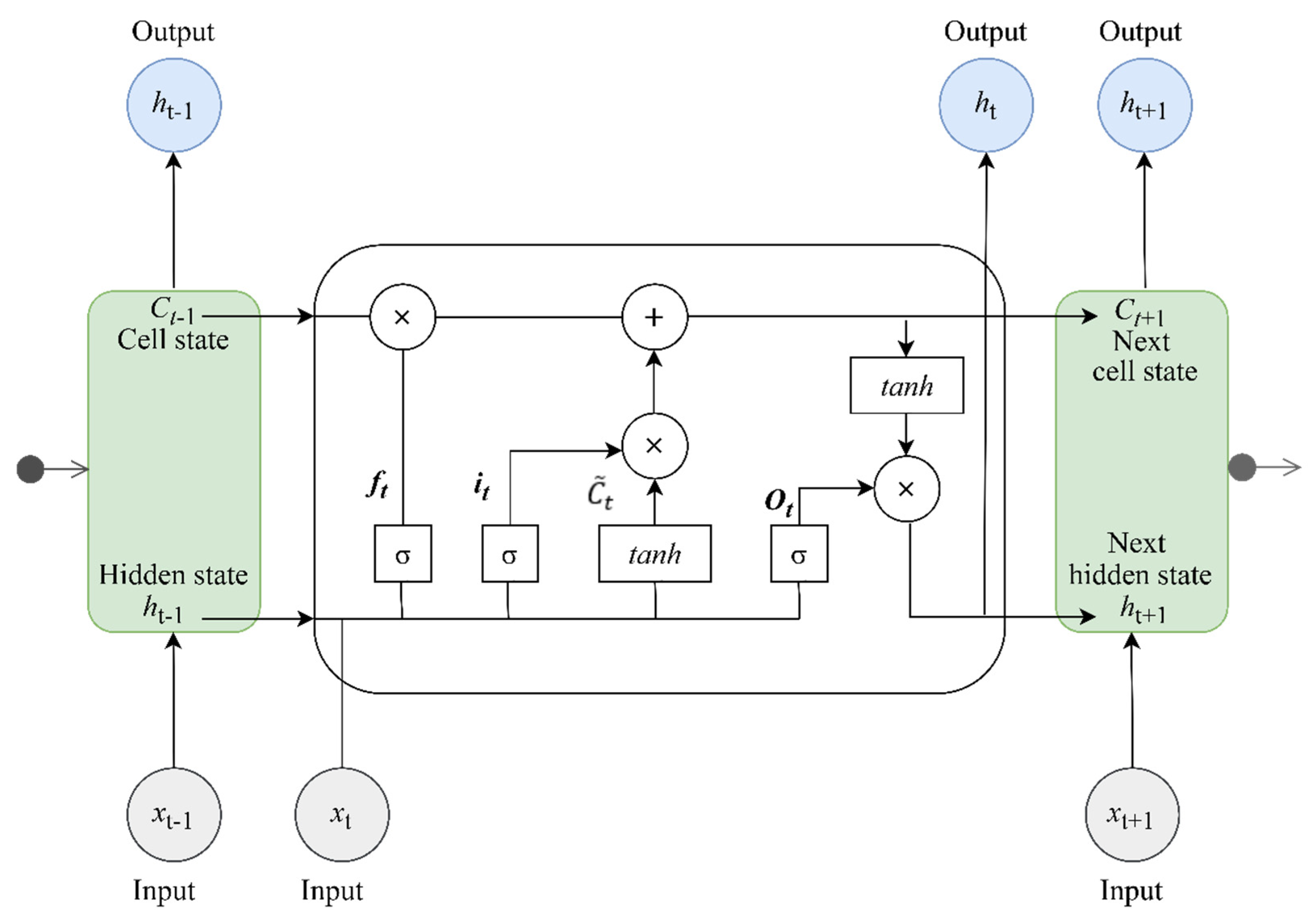
The LSTM network was developed to address the vanishing gradient and exploding challenges in long sequences of data. In the structure of the model, the cell is the basic building block. The cell state employs three gates: input, forget, and output gates. The input gate decides what inputs to allow, the forget gate selects the critical information to keep or discard, and the output gate controls the information passing through. A detailed description of the LSTM architecture (Figure 2) used in this research is given by Dikshit and Pradhan [8]. The model layer encodes sequential information through the recurrent network from the input layer. It outputs a vector with a size of four from a densely connected network that equates to the total number of steps before the forecast. Firstly, when constructing an LSTM, information that is not required should be identified and removed from the cell. The process of information exclusion during identification is usually performed by the sigmoid function, which then returns the output of the final LSTM unit ( h t 1 ) at time t 1 and the present input ( x t ) .
The part of the old output is further eliminated by the sigmoid function ( σ ). This is the first step, and it is regarded as the forget gate ( f t ) , given as follows:
  f t = σ ( ϖ f [ h t 1 ,   x t ] + ϑ f )
where the vector, f t , ranges from 0 to 1, coinciding with the cell state C t 1 . The closer f t is to 0, the more likely that the previous data have been forgotten. Conversely, if the vector is closer to 1, the data are more likely to have been remembered. ϖ f = weight matrices and ϑ f = bias for the forget gate. The second step within the network is to determine which new data from the stage data are to be stored in the cell state (Equation (2)). The σ layer checks what information is to be updated or ignored (1 or 0). The t a n h function (Equation (3)) provides weight to the historical values, thereby determining the degree of significance (from −1 to 1). The information updated by the σ layer and the values decided by t a n h are then multiplied to update the cell state (Equation (4)). The new and old memories are merged with C t 1 , leading to C ˜ t .
i t = σ ( ϖ i   [ h t 1 ,   x t ] + ϑ i )
C ˜ t = t a n h ( ϖ u   [ h t 1 ,   x t ] + ϑ u )
C t = C t 1   f t + C ˜ t i t
where i t = input gate, ϖ i = weights for the input gate, ϑ i = bias for the input gate, ϖ u = updated weights, and ϑ u = updated biases (Equations (2)–(4)). During the third step, the network decides what value to output (Equation (5)). A σ layer is used to determine the output from the cell state. Subsequently, the output values released from the sigmoid gate are multiplied by values generated from the t a n h in the cell state ( C t ) in Equation (6).
O t   = σ ( ϖ o   [ h t 1 ,   x t ] + ϑ o )
  h t = O t t a n h ( C t )
where h t = new output value, O t   = output gate, ϖ o = vector of weights for the output gate, and ϑ o = bias vector for the output gate.
Two approaches are usually used in LSTM for forecasting longer lead times: recursive or direct methods. Here, the direct approach was used, given that the parameters of the previous time step were used to predict future times [48]. A regularization dropout of 0.3 was applied after several trials. A total of 100 neurons were utilized in the LSTM layer and 1 in the dense layer. The model was performed for five timescales, resulting in five LSTM models from each timescale (30, 60, 90, 120, and 180 days). We used the Keras and Scikit-learn application programming interfaces (APIs), which are open-source libraries in the Python programming language, to complete the model building and evaluation.

2.2.2. Transformers

The transformer-based forecasting model used in this research was modeled after [49], which is the classic transformer architecture (Figure 3) with encoder and decoder layers comprising self-attention and fully connected feedforward sublayers. The encoder layer consists of an input, a positional encoder layer, and a stack of up to 6 original interchangeable layers. The input layers delineate the time-series data into a dimension d m o d e l (i.e., delay embedding dimension) via a fully connected network. This is a crucial step in implementing a multi-head attention structure (Figure 3). The sine–cosine functions expressed in Equation (7) were used as the positional encoding for the time series’ sequential information by adding the individual elements of the input vector alongside a positional encoding vector. This encoding was incorporated into the model instead; it was used to furnish each time-series element with information about its position. In short, the model’s input was improved by inserting the time-series data in an orderly manner.
Assuming that x is the position of an element in the time-series data, p x d is the analogous encoding, while d is the dimension of the encoding. Therefore, the function is defined as follows:
p x ( i ) = { sin ( w i . x ) ,   i f   i = 2   cos ( w i . x ) ,   i f   i = 2 + 1
where:
  w i = 1 1000 2 d  
where w i is the frequency for each dimension.
The resulting vector from the positional encoding is fed into four identical encoder layers. The individual encoder layer comprises two sublayers: a fully connected feedforward sublayer ( d f f ) , and a self-attention sublayer. A normalization layer is created after each sublayer. The encoder procedure generates a vector with a delay embedding dimension as an input to the decoder. When using the classical transformer model, there are some limitations posed by the quadratic time complexity with the self-attention procedure and the error of the autoregressive decoder. The informer [50] offers a solution to this problem by introducing a transformer architecture with reduced complexity and a direct multistep forecasting strategy.
The decoder consists of an input layer, four interchangeable decoder layers (Figure 3), and an output layer. The input layer delineates the decoder input from the encoder to a dimension d m o d e l (delay embedding dimension) vector. The decoder incorporates a third sublayer to implement a self-attention mechanism on the output from the encoder. The last decoder layer is then mapped to the time sequence of interest. Here, we ensured that the prediction of the historical data point depends on the past data point by using the look-ahead masking procedure and one positional offset between the input and the output of the decoder.
 i. 
Training
The model was trained to predict hydrological drought for 30, 60, 90, 120, and 180 days into the future from the daily discharge data within a water year between 1928 and 2020 (i.e., 33,602 training days). For example, using the 30-day predictions, the encoder input was given as ( x 1 ,   x 2 , ,   x 33602 ) , with the decoder as ( x 33602 ,   ,   x 33631 ) , where the decoder gave the output ( x 33603 ,   ,   x 33632 ) . The focus was placed on using a look-ahead mask, so the model used the historical data points before the target data. Therefore, while predicting ( x 33603 ,   x 33604 ) , the look-ahead mask makes sure that the weights of attention are applied to ( x 33602 ,   x 33603 ) , preventing the decoder from leaving information about x 33604 ,   ,   x 33632 from the input. A minibatch size (i.e., the number of training examples for one iteration) of 32 was employed during the training.
 ii. 
Optimizer
The RMSProp optimizer is essential in mitigating the rapid decay of the learning rate ( l r ) with the use of “moving averages of squared past gradients” [51]. The gradient-based algorithm is normalized with the squared average moving averages. The normalization often offsets the step size, where the step of large gradients is decreased to avoid exploding, while that of small gradients is increased to prevent vanishing. The optimizer uses an adaptive l r and is not used as a hyperparameter. The l r therefore changes with time. It is given as follows:
E [ g 2 ] t = β E [ g 2 ] t 1 + ( 1 β ) ( δ C δ w ) 2
  w t = w t 1 l r E [ g 2 ] t   δ C δ w
where E [ g ] represents the moving average of squared gradients, δ C δ w is the gradient of the loss function vis-à-vis the weight, l r is the learning rate, and the moving average parameter ( β ) has a default value of 0.9 .
 iii. 
Regularization
The encoder and decoder apply a dropout technique for the three sublayers (self-attention, feed-forward, and normalization). For this model, the dropout value used for each sublayer varies from 0.1 to 0.3 for the different timescales. To build this model, we used the PyTorch and Scikit-learn application programming interfaces (APIs), which are open-source libraries in the Python programming language.

2.2.3. Flood Frequency Analysis

Evaluation of the relationship between the probability and severity of flood or drought is usually characterized by flood frequency distributions derived using a procedure called flood frequency analysis. To identify the stage-height drought level, we adopted the threshold approach first popularized by Yevjevich [52], which is currently in widespread practice. A fixed or variable—i.e., daily, monthly, or seasonal—threshold is usually required. Here, a fixed threshold was adopted, given that the focus was placed on selecting hydrological drought from predicted data from the LSTM and transformer models. A daily threshold level derived from the 75th percentile (75Q) of the daily flow–duration curve (FDC) was applied, with the 70th–95th percentiles commonly used in drought studies for perennial rivers [53].

2.2.4. Model Evaluation

Five models each were built for transformers (TR-30, TR-60, TR-90, TR-120, and TR-180) and LSTM (LSTM-30, LSTM-60, LSTM-90, LSTM-120, and LSTM-180). For both stations, 180 days of data (1 September 2021–27 February 2022) were predicted, and the original values for this period were used as the testing data. Four evaluation metrics were adopted: the mean squared error ( M S E ) , mean absolute error ( M A E ) , root-mean-square error ( R S M E ) , and coefficient of determination ( R 2 ) [6,8,9,54]. The M S E appraises the average squared difference between the observed and forecasted data. M A E measures the errors between paired observations indicating similar phenomena. The R S M E penalizes large errors, where a lower value illustrates good performance, i.e., smaller values signify insufficient errors. The R 2 brings the dispersion from the observed data into clarity, as described by the forecasted data; it ranges from 0 (signifying no correlation between the observed and forecasted data) to 1 (indicating that the distribution of the observed and forecasted data is identical).
M S E = 1 N I 1 N ( x i y i ) 2 ,   0 M A E <
M A E = 1 N i = 1 N | x i y i |   ,   0 M A E <
R S M E = i = 1 N | | x i y i | | 2 N   ,   0   R S M E <
  R 2 = [ i = 1 N ( x i x ¯ ) ( y i y ¯ ) i = 1 N ( ( x i x ¯ ) 2 ) i = 1 N ( y i y ¯ ) 2 ] 2 , 0 R 2 1
where x i is the observed data point with x ¯ as its mean, y i is the forecasted data point with y ¯ as its mean, and N is the total number of observations.
The stage time-series data from 1 October 1928 to 31 August 2021 were used as the training and validation data, where 80% of the data were used for training and 20% for testing. The M S E was used for validating the model using the training and validation samples.

3. Results

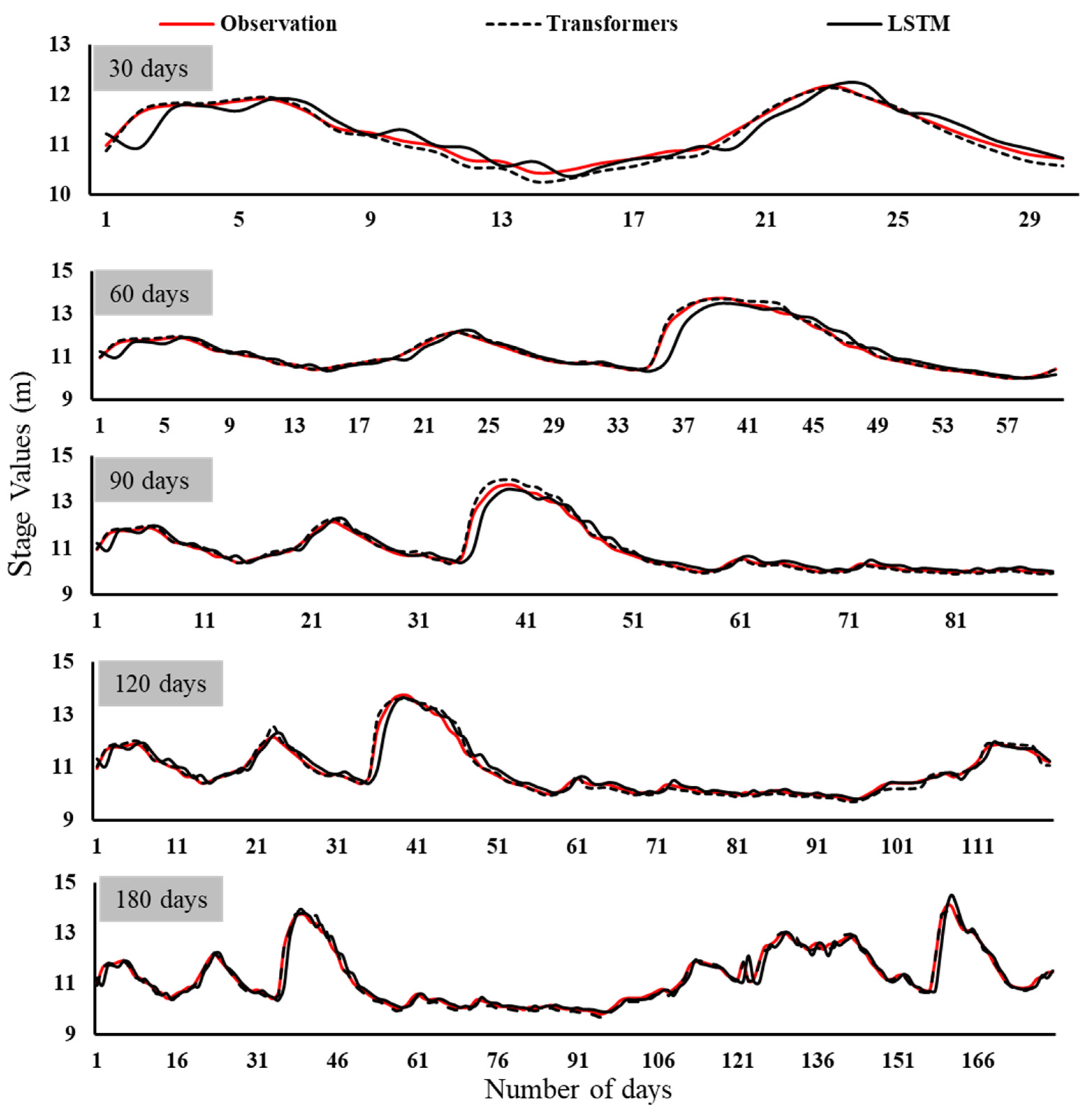
The transformer and LSTM (Figure 4 and Figure 5) models can forecast unseen stage-level data, albeit with variation in outcomes for the different timescales. While running the model, the learning rate varied ( 10 6 to 10 4 ) for the different timescales. There was an observed trend in the stage data, given the changes in water levels within the river because of the Jim Woodruff Dam and other anthropogenic activities on the upper Apalachicola—especially dredging [44,46,55,56].
The DL models predict stage values following the trends and patterns of the data (Figure 4 and Figure 5), but appear to either underestimate (LSTM) or overestimate (transformers) high stage values for all timescales except for the 120-day timescale, where there is variation in underestimation and overestimation for the two models. However, the 60-day forecast for the Chattahoochee station for both models shows some overestimation at high stage values. The transformer model proved to be a better model for predicting longer time series for all periods when comparing the models using the metrics in Table 1. For the most part, the M S E , M A E , and R S M E were closer to 0 than 1, revealing that the forecasted values were more related to the original value, with limited errors. The R 2 for all predictions was generally >90% for transformers and >75% for LSTM, signaling overall good prediction from the DL models. The average values for all metrics are shown in Table 2.
The TR-30 and the TR-120 models showed promising results for both short-term (30 days) and long-term (120 days) forecasts. The 60- and 90-day forecasts for the transformers (TRs) showed that the M S E , M A E , R S M E , and R 2 were not as good as their 30- and 120-day counterparts (Table 2). In contrast, the LSTM models showed high values for these metrics for the 90- and 120-day forecasts, signifying that the transformer models are better for forecasting long-term conditions. For all predictions, the LSTM models performed slightly better than the transformer models when forecasting for 180 days because of the lower values of M S E , M A E , and R S M E and the higher value of R 2 for the LSTM predictions. However, the RMSE for the transformer model showed a better overall performance compared to the LSTM.
The forecasted values of the stage-level historical series from the two stations were then recombined with the original time-series data to help select a daily drought series using a fixed threshold of 75Q.
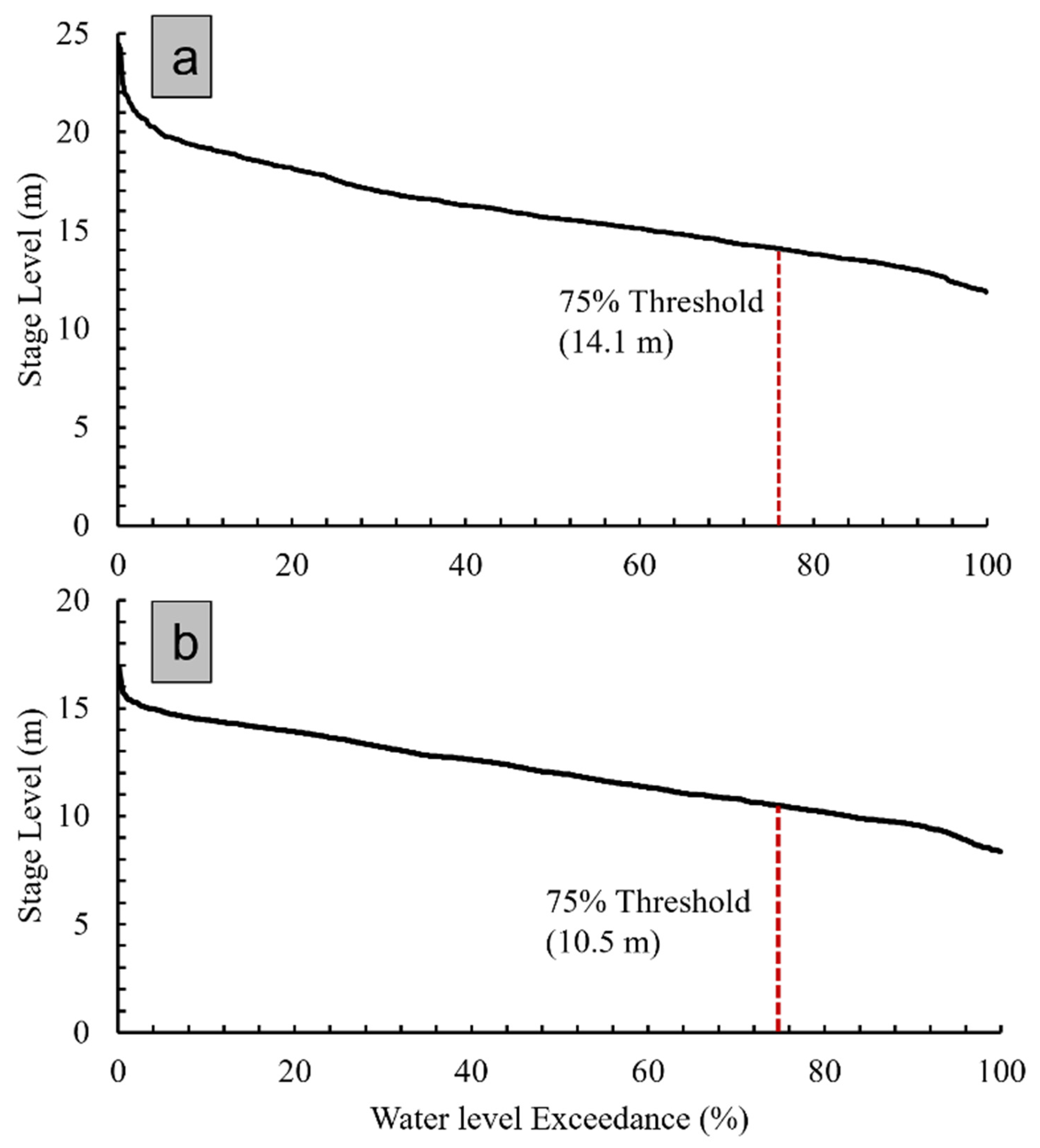
Because the transformers statistically revealed better results, only the predicted values from the TR models were adopted for use in generating the drought series using the flow–duration curves (FDCs) (Figure 6). Given that the TR-120 model produced good results, the predicted values from the model were used to create the drought series for both stations. The threshold stage levels for Chattahoochee and Blountstown were determined to be 14.1 m and 10.5 m, respectively (Figure 6). The resultant threshold calculated using the Weibull formulae [57] revealed that all of the observed data points that equaled or exceeded the truncated level (75Q) exactly matched the counts for those that were forecasted from September to December 2021 using the transformer model (Table 3). When stacking the forecasted water-level data against the observed data, we examined the trend from January 2021 to February 2022 to obtain a visual impression of how the transformer models could replicate the trend (Figure 7). It is clear from the trend that the transformer models performed well in forecasting the pattern of the trend, except for the Chattahoochee station. This could be because the Chattahoochee station is closer to the dam than the Blountstown station.
We examined how many points within the time-series data met the criteria for drought, as well as whether the transformer model predicted those points as drought, by looking at the a c c u r a c y   % = 100 (measured value predicted value 100/measured value) or 100 (predicted value measured value 100/measured value). The percentage accuracy error was determined by querying the total amount of data points that equaled or exceeded the 75Q, meaning how many days within the observed and predicted days were less than 14.1 m and 10.5 m for Chattahoochee and Blountstown, respectively. Table 3 shows the percentage accuracy, revealing how many actual droughts were predicted as droughts by the transformer models, shown as counts and percentages. Most of the hydrological droughts detected in the observed drought series were equally identified in the forecasted drought series, except for Chattahoochee’s 180-day period and Blountstown’s 30-, 90-, 120-, and 180-day periods.
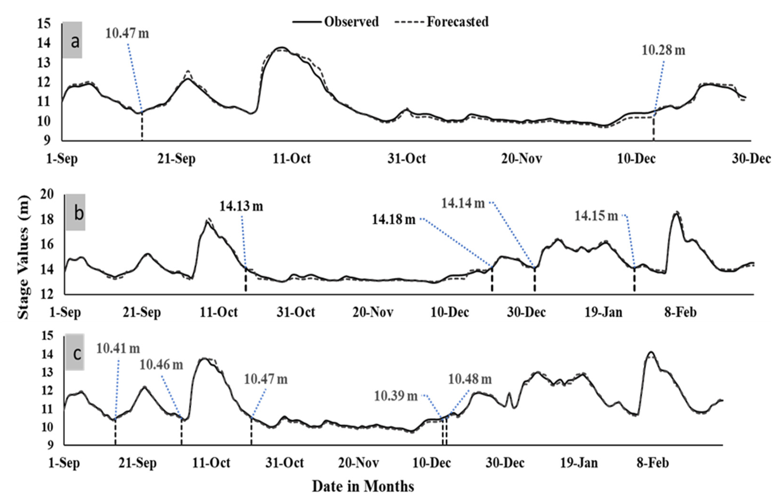
For the case of the 120-day forecast (Figure 8a), the model incorrectly forecasted hydrological drought for 15 September and 13 December (2021) at Blountstown. In addition, the transformer models predicted the occurrence of drought at various points over 180 days (TR-180) within the predicted series when, in truth, there was no actual drought for either the Chattahoochee or Blountstown stations (Figure 8a,b).

4. Discussion

When analyzing drought, many researchers (e.g., [8,12]) initially quantify the hydrological drought with standardized indices (e.g., SPI, SRI) before predicting or forecasting future droughts using a machine or DL model. However, the approach in this study first predicted future data points from the historical data before quantifying drought with the forecasted outcomes from the DL models using the theory of runs, thresholding at 75Q. The advantage of predicting variables before converting to drought series is that unlike computing a monthly, quarterly, or annual hydrological drought series using specified indices, the procedure calculates daily drought series, giving a finer temporal scale for understanding the drought characteristics. The sheer timescale of the hydrological drought series is significant, given that it aids in water resource conservation and management [58]. Daily hydrological drought time series can help in the easy computation of the frequency, magnitude, and duration of drought phenomena within a short timescale [4,59,60]. Furthermore, this research used stage-level data to assess hydrological drought, noting that stage height has a more direct influence on connectivity and inundation [61]—especially for rivers disturbed by anthropogenic activities.
The research compared the transformer and LSTM models, with results showing the superiority of transformer models over LSTM—especially for long-term prediction. The outcomes of this research are consistent with the findings of other studies [28,38] that used DL models for hydrological drought prediction, showing similar quality in the prediction of drought events. For instance, Adikari et al. [38] predicted high runoff values more accurately, since the LSTM models do not overestimate high flow values. This was also true for this study, as the LSTM models predicted high-stage data better than the transformer models. Moreover, Li et al. [28] achieved a high prediction accuracy when comparing the LSTM model to ARIMA, showing the superiority of the LSTM model over the ARIMA model. Although LSTM was proposed to tackle the impact of short-term memory for the better prediction of longer time sequences, the transformer models have an advantage in that they incorporate a seasonal trend decomposition scheme, which can significantly boost prediction outcome by about 50–80% [41]. In addition, while the results of the transformer models are better, the time needed for the individual models to converge and forecast future timestamps is significantly shorter than that for the LSTM models [42], making the transformer models better for predicting future and real-time hydrological drought events. However, the LSTM models performed slightly better than the transformers for predicting a longer lead time (180 days, ~6 months)—especially for the Chattahoochee station, where the models found it difficult to mimic the trend given lower evaluation metrics (Table 2). The lack of accurate depiction of the stage height by the models could arise from the fact that the Chattahoochee station is closer to the Jim Woodruff Dam, which may increase the fluctuation in flow and, consequently, in stage. Dam construction can affect variations in peak discharge and stage levels [62]. It therefore becomes important for future studies to carry out a detailed examination of the degree to which DL models can predict flow or water levels in river ecosystems shaped by human activities.
Based on our results (Figure 4 and Figure 5), the transformer models overestimated some values—especially in areas with a sudden increase in the stage-level data. It was evident that the pattern of the trends for 120 days showed a reducing trend in the f water level, with visible fluctuation—probably due to the possible degradation observed in the upper Apalachicola River [55]. The river has suffered multiple human alterations, including long-term historical dredging, dam construction, irrigation, etc. These human activities affect the stream storage capacity, which is critical for developing and transforming hydrological drought signals, since water storage creates a long-term memory in the hydrological system. The stage data document the cumulative impact of changes upstream as well as the modifications of the channels and floodplain [61]; for this reason, stage-level changes are more noticeable, making the use of stage data very suitable for use in forecasting hydrological drought.
The forecasted hydrological drought values show that over half (>60) of the data points for 1 September 2021–27 February 2022, for both stations, experienced drought (Table 2). The outcome here with respect to drought is not unexpected, given that the drought-defined period from the 75Q for the Apalachicola River is within the window of low rainfall. This result reveals the potential to predict future droughts in a river that shows decreasing flows and stage levels [44,46]. It is clear that the propagation mechanism of hydrological drought is associated with human perturbations in the Apalachicola, such as changes in land use and land cover [63], construction of dams [64,65], dredging [44,46], irrigation water use [66], etc. Specifically, the construction of dams modifies drought propagation, since it has a substantial impact on surface runoff processes. Upstream construction of reservoirs exacerbates the hydrological drought conditions downstream by decreasing flows, favoring locations upstream for water supply, and by decreasing stage levels, further induced by riverbed degradation. Dredging structurally alters several hydraulic variables (e.g., depth, roughness, slope, width) that determine the flow and conveyance capacity, with flood stages typically decreasing, affecting the spatial extent of flood inundation. However, dredging affects stage height differently along the course of the river, revealing disparities in hydrologic processes and water levels along the river’s length.
Although the DL models were successful in the forecasting for the example of the upper Apalachicola River, more studies should be carried out on rivers and drainage basins of different sizes and in different settings. Model performance would be expected to vary with the characteristics of the river and its basin, including the drainage basin area, flashiness, climate, geology, vegetation, tidal influence, anthropogenic activities, and a variety of other factors. Thus, we recommend more testing on a wide variety of rivers. Furthermore, if an unusual event occurred during the prediction period—such as a tropical storm with intense rainfall in what is normally the dry season—it is unknown how well these models would perform.

5. Conclusions

There is frequent drought in the Apalachicola River owing to interannual variations, water consumption battles, and human disturbances. Using stage levels, this paper explored the use of transformer models in predicting drought characteristics. The article benchmarked LSTM for use in comparison with the transformer models. The theory of runs, using a truncation level of 75Q, was adopted to develop hydrological drought series. Four evaluation metrics— M S E , M A E , R S M E , and R 2 —were adopted to compare the transformer and LSTM models against observed values. The main conclusions are as follows:
i.
Evaluation metrics reveal that, on average, the transformer models performed better than the LSTM models across all timestamps for predicting hydrological drought.
ii.
The transformer models overestimated peak stage levels compared to the LSTM models, which accurately forecasted high-stage values.
iii.
The drought series generated from the flow–duration curves (FDCs) were forecasted accurately for the transformer models, except for a few instances in Chattahoochee and Blountstown.
iv.
Water-level data are an important metric for assessing hydrological drought in hydrological systems with increased human pressures.
v.
Although the DL model performed well in this river, model performance would be expected to vary with the characteristics of the river and its basin, including the drainage basin area, flashiness, climate, geology, vegetation, tidal influence, anthropogenic activities, and an array of other factors.
vi.
It is unknown how well the model would perform if there was an unusual event, such as a tropical cyclone passing over the study area during what is typically the dry season.
Hydrological drought research is increasingly becoming an essential domain among hydrologists, given the persistent changes in the complexity of coupled natural and human systems. Deep learning models in the era of big data will be vital for forecasting the magnitude, frequency, and duration of hydrological droughts and developing early-warning systems that help curtail future ecological, agricultural, and socioeconomic losses.

Author Contributions

Conceptualization, A.C.A. and J.M.; methodology, A.C.A.; software, A.C.A.; validation, A.C.A., J.M. and Y.-H.C.; formal analysis, A.C.A.; resources, J.M.; data curation, A.C.A.; writing—original draft preparation, A.C.A.; writing—review and editing, J.M. and Y.-H.C.; visualization, A.C.A. and Y.-H.C.; supervision, J.M.; funding acquisition, J.M. All authors have read and agreed to the published version of the manuscript.

Funding

The data analysis and APC were largely supported by the U.S. Environmental Protection Agency (EPA), Gulf of Mexico Program Project P0078306: Stabilizing Point Bars on Apalachicola River (J. Mossa, PI); project manager: Jerry Binninger. The content of this article is solely the responsibility of the authors and does not necessarily represent the official views of the EPA.

Data Availability Statement

The data for this research was collected from United States Geological Survey (USGS) and can be downloaded here https://waterdata.usgs.gov/nwis, available on 12 October 2022.

Acknowledgments

We would like to express our thanks to the Department of Geography’s GeoAI and STAR Laboratory for providing the computing system and resources for the completion of the research.

Conflicts of Interest

The authors declare no conflict of interest.

References

  1. Mind’je, R.; Li, L.; Amanambu, A.C.; Nahayo, L.; Nsengiyumva, J.B.; Gasirabo, A.; Mindje, M. Flood Susceptibility Modeling and Hazard Perception in Rwanda. Int. J. Disaster Risk Reduct. 2019, 38, 101211. [Google Scholar] [CrossRef]
  2. Tu, X.; Wu, H.; Singh, V.P.; Chen, X.; Lin, K.; Xie, Y. Multivariate Design of Socioeconomic Drought and Impact of Water Reservoirs. J. Hydrol. 2018, 566, 192–204. [Google Scholar] [CrossRef]
  3. Mishra, A.K.; Singh, V.P. A Review of Drought Concepts. J. Hydrol. 2010, 391, 202–216. [Google Scholar] [CrossRef]
  4. Van Loon, A.F. Hydrological Drought Explained. WIREs Water 2015, 2, 359–392. [Google Scholar] [CrossRef]
  5. Almikaeel, W.; Čubanová, L.; Šoltész, A. Hydrological Drought Forecasting Using Machine Learning—Gidra River Case Study. Water 2022, 14, 387. [Google Scholar] [CrossRef]
  6. Achite, M.; Jehanzaib, M.; Elshaboury, N.; Kim, T.-W. Evaluation of Machine Learning Techniques for Hydrological Drought Modeling: A Case Study of the Wadi Ouahrane Basin in Algeria. Water 2022, 14, 431. [Google Scholar] [CrossRef]
  7. Agana, N.A.; Homaifar, A. A Deep Learning Based Approach for Long-Term Drought Prediction. In Proceedings of the SoutheastCon 2017, Charlotte, NC, USA, 30 March–2 April 2017; pp. 1–8. [Google Scholar]
  8. Dikshit, A.; Pradhan, B. Explainable AI in Drought Forecasting. Mach. Learn. Appl. 2021, 6, 100192. [Google Scholar] [CrossRef]
  9. Jehanzaib, M.; Shah, S.A.; Yoo, J.; Kim, T.-W. Investigating the Impacts of Climate Change and Human Activities on Hydrological Drought Using Non-Stationary Approaches. J. Hydrol. 2020, 588, 125052. [Google Scholar] [CrossRef]
  10. Maity, R.; Khan, M.I.; Sarkar, S.; Dutta, R.; Maity, S.S.; Pal, M.; Chanda, K. Potential of Deep Learning in Drought Assessment by Extracting Information from Hydrometeorological Precursors. J. Water Clim. Chang. 2021, 12, 2774–2796. [Google Scholar] [CrossRef]
  11. Nabipour, N.; Dehghani, M.; Mosavi, A.; Shamshirband, S. Short-Term Hydrological Drought Forecasting Based on Different Nature-Inspired Optimization Algorithms Hybridized With Artificial Neural Networks. IEEE Access 2020, 8, 15210–15222. [Google Scholar] [CrossRef]
  12. Wang, G.C.; Zhang, Q.; Band, S.S.; Dehghani, M.; Chau, K.W.; Tho, Q.T.; Zhu, S.; Samadianfard, S.; Mosavi, A. Monthly and Seasonal Hydrological Drought Forecasting Using Multiple Extreme Learning Machine Models. Eng. Appl. Comput. Fluid Mech. 2022, 16, 1364–1381. [Google Scholar] [CrossRef]
  13. McKee, T.B.; Doesken, N.J.; Kleist, J. The Relationship of Drought Frequency and Duration to Time Scales. In Proceedings of the 8th Conference on Applied Climatology, Anaheim, CA, USA, 17–22 January 1993. [Google Scholar]
  14. Nalbantis, I.; Tsakiris, G. Assessment of Hydrological Drought Revisited. Water Resour. Manag. 2009, 23, 881–897. [Google Scholar] [CrossRef]
  15. Garen, D.C. Revised Surface-Water Supply Index for Western United States. J. Water Resour. Plan. Manag. 1993, 119, 437–454. [Google Scholar] [CrossRef]
  16. Vicente-Serrano, S.M.; Beguería, S.; López-Moreno, J.I. A Multiscalar Drought Index Sensitive to Global Warming: The Standardized Precipitation Evapotranspiration Index. J. Clim. 2010, 23, 1696–1718. [Google Scholar] [CrossRef] [Green Version]
  17. Shukla, S.; Wood, A.W. Use of a Standardized Runoff Index for Characterizing Hydrologic Drought. Geophys. Res. Lett. 2008, 35, L02405. [Google Scholar] [CrossRef] [Green Version]
  18. Alley, W.M. The Palmer Drought Severity Index: Limitations and Assumptions. J. Appl. Meteorol. Climatol. 1984, 23, 1100–1109. [Google Scholar] [CrossRef]
  19. Narasimhan, B.; Srinivasan, R. Development and Evaluation of Soil Moisture Deficit Index (SMDI) and Evapotranspiration Deficit Index (ETDI) for Agricultural Drought Monitoring. Agric. For. Meteorol. 2005, 133, 69–88. [Google Scholar] [CrossRef]
  20. Dehghani, M.; Saghafian, B.; Zargar, M. Probabilistic Hydrological Drought Index Forecasting Based on Meteorological Drought Index Using Archimedean Copulas. Hydrol. Res. 2019, 50, 1230–1250. [Google Scholar] [CrossRef]
  21. Liu, Z.; Wang, Y.; Xu, Z.; Duan, Q. Conceptual Hydrological Models. In Handbook of Hydrometeorological Ensemble Forecasting; Duan, Q., Pappenberger, F., Thielen, J., Wood, A., Cloke, H.L., Schaake, J.C., Eds.; Springer: Berlin/Heidelberg, Germany, 2017; pp. 1–23. ISBN 978-3-642-40457-3. [Google Scholar]
  22. Shirmohammadi, B.; Moradi, H.; Moosavi, V.; Semiromi, M.T.; Zeinali, A. Forecasting of Meteorological Drought Using Wavelet-ANFIS Hybrid Model for Different Time Steps (Case Study: Southeastern Part of East Azerbaijan Province, Iran). Nat. Hazards 2013, 69, 389–402. [Google Scholar] [CrossRef]
  23. Belayneh, A.; Adamowski, J. Drought Forecasting Using New Machine Learning Methods. J. Water Land Dev. 2013, 18, 3–12. [Google Scholar] [CrossRef]
  24. Mokhtarzad, M.; Eskandari, F.; Jamshidi Vanjani, N.; Arabasadi, A. Drought Forecasting by ANN, ANFIS, and SVM and Comparison of the Models. Environ. Earth Sci. 2017, 76, 729. [Google Scholar] [CrossRef]
  25. Bazrafshan, O.; Salajegheh, A.; Bazrafshan, J.; Mahdavi, M.; Fatehi Maraj, A. Hydrological Drought Forecasting Using ARIMA Models (Case Study: Karkheh Basin). ECOPERSIA 2015, 3, 1099–1117. [Google Scholar]
  26. Dikshit, A.; Pradhan, B.; Alamri, A.M. Temporal Hydrological Drought Index Forecasting for New South Wales, Australia Using Machine Learning Approaches. Atmosphere 2020, 11, 585. [Google Scholar] [CrossRef]
  27. Hao, Z.; Hao, F.; Singh, V.P.; Sun, A.Y.; Xia, Y. Probabilistic Prediction of Hydrologic Drought Using a Conditional Probability Approach Based on the Meta-Gaussian Model. J. Hydrol. 2016, 542, 772–780. [Google Scholar] [CrossRef]
  28. Li, Y.; Wang, B.; Gong, Y. Drought Assessment Based on Data Fusion and Deep Learning. Comput. Intell. Neurosci. 2022, 2022, 4429286. [Google Scholar] [CrossRef]
  29. Shamshirband, S.; Hashemi, S.; Salimi, H.; Samadianfard, S.; Asadi, E.; Shadkani, S.; Kargar, K.; Mosavi, A.; Nabipour, N.; Chau, K.-W. Predicting Standardized Streamflow Index for Hydrological Drought Using Machine Learning Models. Eng. Appl. Comput. Fluid Mech. 2020, 14, 339–350. [Google Scholar] [CrossRef]
  30. Sharma, T.C.; Panu, U.S. Prediction of Hydrological Drought Durations Based on Markov Chains: Case of the Canadian Prairies. Hydrol. Sci. J. 2012, 57, 705–722. [Google Scholar] [CrossRef] [Green Version]
  31. Sattar, M.N.; Lee, J.-Y.; Shin, J.-Y.; Kim, T.-W. Probabilistic Characteristics of Drought Propagation from Meteorological to Hydrological Drought in South Korea. Water Resour. Manag. 2019, 33, 2439–2452. [Google Scholar] [CrossRef]
  32. Bae, D.-H.; Son, K.-H.; So, J.-M. Utilization of the Bayesian Method to Improve Hydrological Drought Prediction Accuracy. Water Resour. Manag. 2017, 31, 3527–3541. [Google Scholar] [CrossRef]
  33. Jehanzaib, M.; Shah, S.A.; Son, H.J.; Jang, S.-H.; Kim, T.-W. Predicting Hydrological Drought Alert Levels Using Supervised Machine-Learning Classifiers. KSCE J. Civ. Eng. 2022, 26, 3019–3030. [Google Scholar] [CrossRef]
  34. Aghelpour, P.; Bahrami-Pichaghchi, H.; Varshavian, V. Hydrological Drought Forecasting Using Multi-Scalar Streamflow Drought Index, Stochastic Models and Machine Learning Approaches, in Northern Iran. Stoch. Environ. Res. Risk Assess. 2021, 35, 1615–1635. [Google Scholar] [CrossRef]
  35. Malik, A.; Kumar, A.; Singh, R.P. Application of Heuristic Approaches for Prediction of Hydrological Drought Using Multi-Scalar Streamflow Drought Index. Water Resour. Manag. 2019, 33, 3985–4006. [Google Scholar] [CrossRef]
  36. Rose, M.A.J.; Chithra, N.R. Tree-Based Ensemble Model Prediction for Hydrological Drought in a Tropical River Basin of India. Int. J. Environ. Sci. Technol. 2022, 1–18. [Google Scholar] [CrossRef]
  37. Anshuka, A.; Chandra, R.; Buzacott, A.J.V.; Sanderson, D.; van Ogtrop, F.F. Spatio Temporal Hydrological Extreme Forecasting Framework Using LSTM Deep Learning Model. Stoch. Environ. Res. Risk Assess. 2022, 36, 3467–3485. [Google Scholar] [CrossRef]
  38. Adikari, K.E.; Shrestha, S.; Ratnayake, D.T.; Budhathoki, A.; Mohanasundaram, S.; Dailey, M.N. Evaluation of Artificial Intelligence Models for Flood and Drought Forecasting in Arid and Tropical Regions. Environ. Model. Softw. 2021, 144, 105136. [Google Scholar] [CrossRef]
  39. Salleh, M.N.M.; Talpur, N.; Hussain, K. Adaptive Neuro-Fuzzy Inference System: Overview, Strengths, Limitations, and Solutions. In Proceedings of the International Conference on Data Mining and Big Data, Fukuoka, Japan, 27 July–1 August 2017; Tan, Y., Takagi, H., Shi, Y., Eds.; Springer International Publishing: Cham, Switzerland, 2017; pp. 527–535. [Google Scholar]
  40. Yaseen, Z.M.; Sulaiman, S.O.; Deo, R.C.; Chau, K.-W. An Enhanced Extreme Learning Machine Model for River Flow Forecasting: State-of-the-Art, Practical Applications in Water Resource Engineering Area and Future Research Direction. J. Hydrol. 2019, 569, 387–408. [Google Scholar] [CrossRef]
  41. Wen, Q.; Zhou, T.; Zhang, C.; Chen, W.; Ma, Z.; Yan, J.; Sun, L. Transformers in Time Series: A Survey. arXiv 2022, arXiv:2202.07125. [Google Scholar]
  42. Wu, H.; Xu, J.; Wang, J.; Long, M. Autoformer: Decomposition Transformers with Auto-Correlation for Long-Term Series Forecasting. Adv. Neural Inf. Process. Syst. 2022, 34, 22419–22430. [Google Scholar]
  43. Minixhofer, C.; Swan, M.; McMeekin, C.; Andreadis, P. DroughtED: A Dataset and Methodology for Drought Forecasting Spanning Multiple Climate Zones. In Proceedings of the Tackling Climate Change with Machine Learning: Workshop at ICML, Gainesville, FL, USA, 23–24 July 2021; p. 9. [Google Scholar]
  44. Light, H.M.; Vincent, K.R.; Darst, M.R.; Price, F.D. Water-Level Decline in the Apalachicola River, Florida, from 1954 to 2004, and Effects on Floodplain Habitats; Scientific Investigations Report; U.S. Geological Survey: Tallahassee, FL, USA, 2006; Volume 2006–5173, p. 61. [Google Scholar]
  45. Smith, M.C.; Anthony Stallins, J.; Maxwell, J.T.; Van Dyke, C. Hydrological Shifts and Tree Growth Responses to River Modification along the Apalachicola River, Florida. Phys. Geogr. 2013, 34, 491–511. [Google Scholar] [CrossRef]
  46. Mossa, J.; Chen, Y.-H.; Kondolf, G.M.; Walls, S.P. Channel and Vegetation Recovery from Dredging of a Large River in the Gulf Coastal Plain, USA. Earth Surf. Process. Landf. 2020, 45, 1926–1944. [Google Scholar] [CrossRef]
  47. Chen, Y.-H.; Mossa, J.; Singh, K.K. Floodplain Response to Varied Flows in a Large Coastal Plain River. Geomorphology 2020, 354, 107035. [Google Scholar] [CrossRef]
  48. Mishra, A.K.; Desai, V.R. Drought Forecasting Using Feed-Forward Recursive Neural Network. Ecol. Model. 2006, 198, 127–138. [Google Scholar] [CrossRef]
  49. Vaswani, A.; Shazeer, N.; Parmar, N.; Uszkoreit, J.; Jones, L.; Gomez, A.N.; Kaiser, Ł.; Polosukhin, I. Attention Is All You Need. In Proceedings of the Advances in Neural Information Processing Systems, Long Beach, CA, USA, 4–9 December 2017; Curran Associates, Inc.: Red Hook, NY, USA, 2017; Volume 30. [Google Scholar]
  50. Zhou, H.; Zhang, S.; Peng, J.; Zhang, S.; Li, J.; Xiong, H.; Zhang, W. Informer: Beyond Efficient Transformer for Long Sequence Time-Series Forecasting. In Proceedings of the AAAI Conference on Artificial Intelligence, Virtual, 22 February–1 March 2021. [Google Scholar]
  51. Zou, F.; Shen, L.; Jie, Z.; Zhang, W.; Liu, W. A Sufficient Condition for Convergences of Adam and RMSProp. In Proceedings of the IEEE/CVF Conference on Computer Vision and Pattern Recognition 2019, Long Beach, CA, USA, 15–16 June 2019; pp. 11127–11135. [Google Scholar]
  52. Yevjevich, V. An Objective Approach to Definitions and Investigations of Continental Hydrologic Droughts. J. Hydrol. 1969, 7, 353. [Google Scholar] [CrossRef]
  53. Tallaksen, L.M.; Hisdal, H.; Lanen, H.A.J.V. Space–Time Modelling of Catchment Scale Drought Characteristics. J. Hydrol. 2009, 375, 363–372. [Google Scholar] [CrossRef]
  54. Elshaboury, N.; Marzouk, M. Comparing Machine Learning Models For Predicting Water Pipelines Condition. In Proceedings of the 2020 2nd Novel Intelligent and Leading Emerging Sciences Conference (NILES), Giza, Egypt, 24–26 October 2020; pp. 134–139. [Google Scholar]
  55. Mossa, J.; Chen, Y.-H. Geomorphic Response to Historic and Ongoing Human Impacts in a Large Lowland River. Earth Surf. Process. Landf. 2022, 47, 1550–1569. [Google Scholar] [CrossRef]
  56. Mossa, J.; Chen, Y.-H. Geomorphic Insights from Eroding Dredge Spoil Mounds Impacting Channel Morphology. Geomorphology 2021, 376, 107571. [Google Scholar] [CrossRef]
  57. Ward, A.; Trimble, S.; Buckrard, S.; Lyon, S. Environmental Hydrology, 3rd ed.; Taylor and Francis Group: Abingdon, UK, 2016; ISBN 978-1-4665-8941-4. [Google Scholar]
  58. Rivera, J.A.; Araneo, D.C.; Penalba, O.C. Threshold Level Approach for Streamflow Drought Analysis in the Central Andes of Argentina: A Climatological Assessment. Hydrol. Sci. J. 2017, 62, 1949–1964. [Google Scholar] [CrossRef]
  59. Tallaksen, L.M.; Hisdal, H.E.G.E. Regional Analysis of Extreme Streamflow Drought Duration and Deficit Volume. IAHS Publ. 1997, 246, 141–150. [Google Scholar]
  60. Van Loon, A.F.; Van Lanen, H.A.J. A Process-Based Typology of Hydrological Drought. Hydrol. Earth Syst. Sci. 2012, 16, 1915–1946. [Google Scholar] [CrossRef] [Green Version]
  61. Pinter, N.; Ickes, B.S.; Wlosinski, J.H.; van der Ploeg, R.R. Trends in Flood Stages: Contrasting Results from the Mississippi and Rhine River Systems. J. Hydrol. 2006, 331, 554–566. [Google Scholar] [CrossRef]
  62. Graf, W.L. Downstream Hydrologic and Geomorphic Effects of Large Dams on American Rivers. Geomorphology 2006, 79, 336–360. [Google Scholar] [CrossRef]
  63. Hovenga, P.A.; Wang, D.; Medeiros, S.C.; Hagen, S.C.; Alizad, K. The Response of Runoff and Sediment Loading in the Apalachicola River, Florida to Climate and Land Use Land Cover Change. Earths Future 2016, 4, 124–142. [Google Scholar] [CrossRef] [Green Version]
  64. Elder, J.F.; Flagg, S.D.; Mattraw, H.C., Jr. Hydrology and Ecology of the Apalachicola River, Florida: A Summary of the River Quality Assessment; U.S. Government Publishing Office: Washington, DC, USA, 1988.
  65. Joshi, S. Long Term Hydrological Changes in the Apalachicola River, Florida. Int. J. Environ. Sci. Nat. Resour. 2019, 19, 152–159. [Google Scholar] [CrossRef]
  66. Piqué, G.; Batalla, R.J.; Sabater, S. Hydrological Characterization of Dammed Rivers in the NW Mediterranean Region. Hydrol. Process. 2016, 30, 1691–1707. [Google Scholar] [CrossRef]
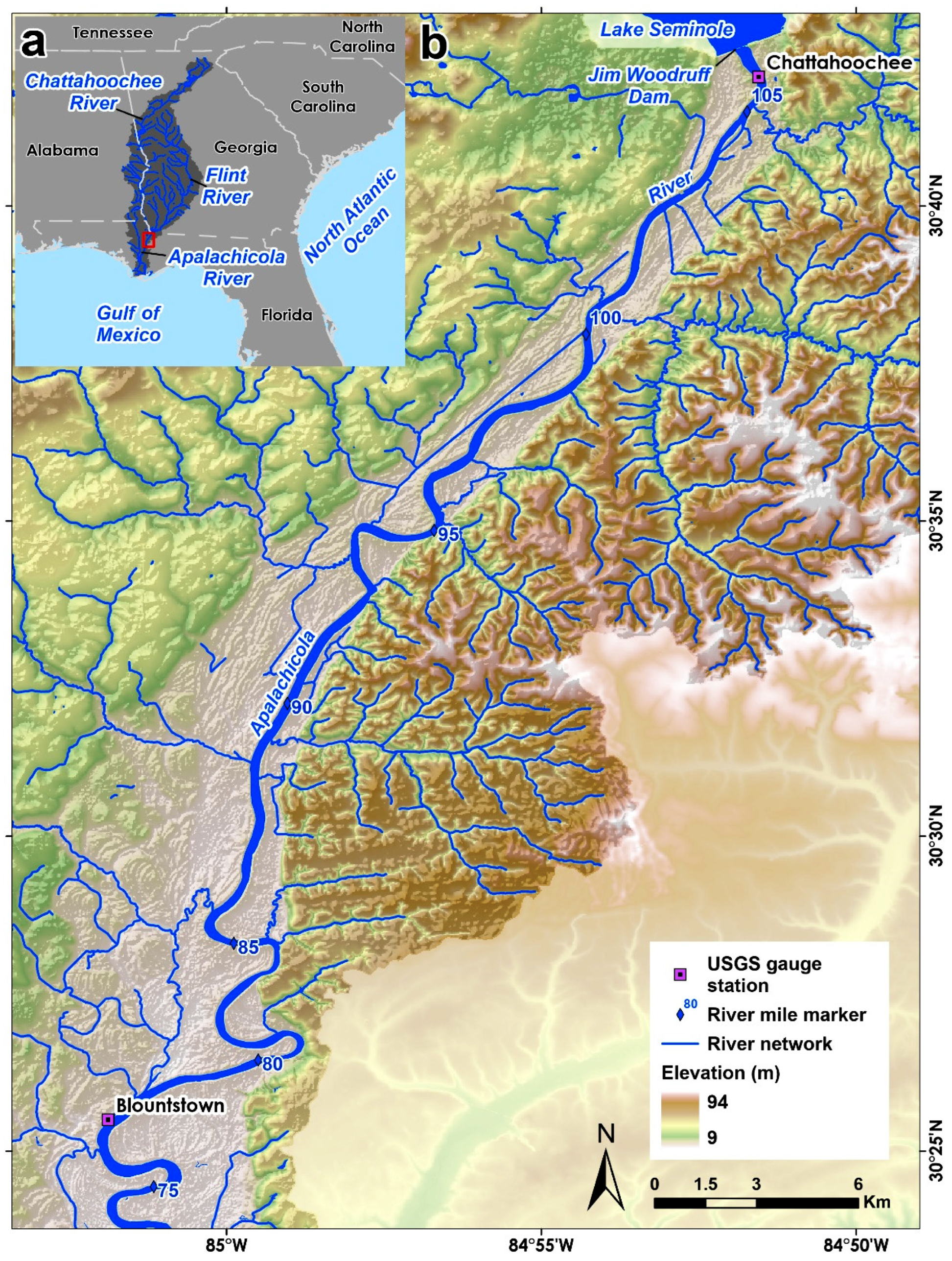
Figure 1. Study area map showing floodplain elevation, USGS gauge stations, and river mile markers of the upper Apalachicola River (b), which is part of the ACF basin (a).
Water 14 03611 g001
Figure 2. A diagram demonstrating the structure of the LSTM (modified from Li et al. [32]).
Water 14 03611 g002
Figure 3. A diagram showing the architecture for the transformer model with four encoder–decoder layers.
Water 14 03611 g003
Figure 4. Outcomes of the DL models vs. different future forecasted stage data for Chattahoochee station.
Water 14 03611 g004
Figure 5. Results of DL models vs, different future forecasted stage data for Blountstown station.
Water 14 03611 g005
Figure 6. Water level exceedance probabilities for the Chattahoochee (a) and Blountstown (b) stations.
Water 14 03611 g006
Figure 7. Combined observed and forecasted stage data for Chattahoochee (a) and Blountstown (b).
Water 14 03611 g007
Figure 8. Observed vs. forecasted values: 120 days for Blountstown (a), 180 days for Chattahoochee (b), and 180 days for Blountstown (c). The values in panels (a,b) show where the transformer models predicted drought across several months but there was no drought for that specific point on that date.
Water 14 03611 g008
Table 2. Performance of transformer and LSTM models for stage-level (m) data.
Performance Indicators
DL Model Timescale (Days)ChattahoocheeBlountstown
M S E M A E R M S E R2MSE M A E R M S E R2
Transformers300.020.120.140.900.020.120.150.91
600.120.260.350.890.040.150.180.92
900.120.200.350.940.080.260.330.92
1200.040.120.210.920.050.170.220.93
1800.230.370.480.960.090.250.290.97
Average 0.1060.2140.3060.9220.0560.1900.2340.930
LSTM300.070.200.260.770.040.170.210.85
600.140.280.380.850.110.210.320.87
900.160.330.400.920.060.160.260.89
1200.080.150.280.900.050.230.230.89
1800.140.180.370.870.070.150.260.94
Average 0.1180.2280.3380.8620.0660.1840.2560.888
Table 3. Percentage accuracy of hydrological drought detected by the transformer models.
ChattahoocheeBlountstown
Count (Drought Days) Count (Drought Days)
ModelObservedPredicted% Accuracy ObservedPredicted% Accuracy
TR-3016161007885.7
TR-6032321002222100
TR-906060100524688.5
TR-1208282100525496.2
TR-180949895.7525790.4
Publisher’s Note: MDPI stays neutral with regard to jurisdictional claims in published maps and institutional affiliations.