On the Numerical Solution of Sparse Linear Systems Emerging in Finite Volume Discretizations of 2D Boussinesq-Type Models on Unstructured Grids

Abstract

This work aims to supplement the realization and validation of a higher-order well-balanced unstructured finite volume (FV) scheme, that has been relatively recently presented, for numerically simulating weakly non-linear weakly dispersive water waves over varying bathymetries. We investigate and develop solution strategies for the sparse linear system that appears during this FV discretisation of a set of extended Boussinesq-type equations on unstructured meshes. The resultant linear system of equations must be solved at each discrete time step as to recover the actual velocity field of the flow and advance in time. The system’s coefficient matrix is sparse, un-symmetric and often ill-conditioned. Its characteristics are affected by physical quantities of the problem to be solved, such as the undisturbed water depth and the mesh topology. To this end, we investigate the application of different well-known iterative techniques, with and without the usage of preconditioners and reordering, for the solution of this sparse linear system. The iiterative methods considered are the GMRES and the BiCGSTAB, three preconditioning techniques, including different ILU factorizations and two different reordering techniques are implemented and discussed. An optimal strategy, in terms of computational efficiency and robustness, is finally proposed which combines the use of the BiCGSTAB method with the ILUT preconditioner and the Reverse Cuthill–McKee reordering.

1. Introduction

Boussinesq-type (BT) equations have been widely used in the past few decades for the description of water wave propagation and transformation near coastal zones. Starting from the classical Boussinesq equations [1], which are limited to relatively shallow water, and up to now-days, numerous researchers have contributed to the development of analytical theories and their numerical approximation as to simulate the various wave phenomena such as wave shoaling, diffraction, refraction and breaking. As such, significant attempts have been made to extend the applicability of the Boussinesq-type models to deeper water, for example in [2,3,4]. These extended models give a more accurate representation of the wave’s phase and group velocities in intermediate waters, with water depth to wavelength ratio up to 1/2, and sometimes are referred to as low-order enhanced BT equations. Moreover, significant effort has been made in recent years into advancing the nonlinear and dispersive properties of BT models by including high-order nonlinear and dispersion terms, we refer for example to [5,6,7,8]. An extensive review, which describes the state of the art in water wave modeling by means of BT models, can be found, for example, in [9].

For the numerical solution of BT equations different methods have been proposed such as, the Finite-Difference (FD) method, [3,4,8,10] and the Finite-Element method, [11,12,13]. In the last ten years the use of the Finite-Volume (FV) method has become the most widely used one due to its effectiveness in the approximation of hyperbolic conservation laws. Applications and advances along this line of research can be found, for example, in [14,15,16,17,18,19,20,21,22]. Usually in the numerical solution of BT equations the inversion of one or more matrices, i.e., solution(s) of linear system(s), is required as to recover the actual velocity field of the water flow from the solution variables. This is an essential procedure (especially in two-dimensional simulations) if the original dispersive BT equations are re-written in a conservative-like form and the vector of the unknown variables includes part of the dispersive terms, [9]. In the most simple cases e.g., when structured computational meshes are used, the linear system’s matrices can be of tridiagonal shape, but when using e.g., unstructured meshes the matrices that occur are more complicated, unsymmetric and have variable sparsity patterns [10,12,19]. For this reason further investigations for the efficient and accurate solution of the resulting linear systems in two-dimensional computations on unstructured meshes are in needed.

This work is complementary to [19,20,23] where, for the first time, a high-order well-balanced unstructured finite volume (FV) scheme on triangular meshes was presented for modeling weakly nonlinear and weakly dispersive water waves over slowly varying bathymetries, as described by the 2D depth-integrated extended Boussinesq equations of Nwogu [3] rewritten in conservation law form. Formulating the model equations in conservative form is imperative when one wants to exploit the advantages modern FV schemes have to offer, such as conservativity and shock-capturing. In this work, the FV scheme implemented numerically solves the conservative form of the equations, following the median dual node-centered approach, for both the advective and dispersive part of the equations. For the advective fluxes, the scheme utilizes an approximate Riemann solver along with a well-balanced topography source term upwinding. Higher order accuracy in space and time is achieved through a MUSCL-type reconstruction technique and through a strong stability preserving explicit Runge–Kutta time stepping. After each step in the time marching scheme a non-trivial sparse linear system must be solved in order to recover the velocity field in the flow. To this end, the accuracy and efficiency of the overall numerical solver depends on this system’s solution.

Following from the above, we examine here, in some depth, the solution process that must be followed for the solution of this sparse and large linear system. The complexity of the system is such that the use of iterative methods is necessary to obtain efficient solutions for even moderately sized problems (depending on the degrees of freedom). As such, two classical Krylov Subspace iterative methods are utilized in this work [24,25]. The Generalized Minimal Residual (GMRES) and the Biconjucate Gradient Stabilized (BiCGStab) algorithms. Both methods are implemented using the SPARSKIT package [26]. The optimal solution strategy depends on factors such as problem size, sparsity pattern and the system’s matrix eigenspectrum. The applicability of these two well-known iterative methods along with preconditioning and reordering possibilities are examined, as to find an efficient solution procedure. The effect of the mesh’s topology and of certain physical conditions, e.g., the flow field’s reference water depth, to the solution procedure is also investigated. We deem that the investigation will provide the useful guidelines needed when other such model equations are to be approximated on unstructured meshes and by any FV numerical approach. This we consider to be the major novel aspect of the present work.

The outline of this paper is as follows: The BT model equations are described in Section 2 while the numerical model used is briefly presented in Section 3 along with the derivation of the sparse matrix and its properties. The iterative methods utilized for the solution of the resulting linear system, the preconditioning methods tested and a detailed comparison of their performance are presented in Section 4, while Section 5 describes the reordering methods. Conclusions are drawn in Section 6.

2. Governing Equations

A number of BT models have been developed to describe the transformation and propagation of waves in coastal regions. In this work, the model equations solved are the extended BT equations of Nwogu [3] which are based on the assumption that the wave height $\left(A\right)$ is much smaller that the water depth h. The equations derived by Nwogu [3] using the velocity vector ${[u,v]}^{\mathrm{T}}=\mathbf{u}\equiv {\mathbf{u}}_a$ at an arbitrary distance, $z_a$, from a still water level, h, as the velocity variable, instead of the commonly used depth-averaged velocity. The elevation of the velocity variable $z_a$ becames a free parameter used to optimize the equations and making them applicable to a wider range of water depths, compared to the classical Boussinesq equations. The equations of Nwogu describe weakly non-linear and weakly dispersive water waves in variable water depth. $ϵ:=A/h$, which measures the weight of nonlinear effects, and the square water depth to wave length (L) ratio ${\mu }^2:=h^2/L^2$, which represents the dimension of the dispersive effects, is of the same order with, i.e., the Stokes number $S:=ϵ/{\mu }^2=O\left(1\right)$. The equations provide accurate linear dispersion and shoaling characteristics for values of $kh\approx 3$ (intermediate water depths), where k is the wave number and $kh$ is essentially a scale of the value of $\mu$, providing a correction of $O\left({\mu }^2\right)$ to the shallow water theory. The equations are presented here in a conservative-like form and as such are numerically approximated by an unstructured FV scheme. Following [19] the vector conservative form of the equations reads as:

$${\partial }_t\mathbf{U}+\nabla ·\mathcal{H}\left({\mathbf{U}}^{☆}\right)=\mathbf{S}\mathrm{on}\mathrm{\Omega }\times [0,t]\subset {\mathbb{R}}^2\times {\mathbb{R}}^{+},$$

(1)

where $\mathrm{\Omega }\times [0,t]$ is the space-time Cartesian domain over which solutions are sought, ${\mathbf{U}}^{☆}={[H,Hu,Hv]}^{\mathrm{T}}$ are the physically conservative variables, $\mathbf{U}$ is the vector of the actual solution variables, with H being the total water depth and $\mathcal{H}=[\mathbf{F},\mathbf{G}]$ are the nonlinear flux vectors given as

$$\mathbf{U}=\left[\begin{array}{c}H\\ P_1\\ P_2\end{array}\right],\mathbf{F}=\left[\begin{array}{c}Hu\\ H{u}^2+\frac{1}{2}g{H}^2\\ Huv\end{array}\right],\mathbf{G}=\left[\begin{array}{c}Hv\\ Huv\\ H{v}^2+\frac{1}{2}g{H}^2\end{array}\right],$$

where

$$\mathbf{P}=\left[\begin{array}{c}P1\\ P2\end{array}\right]=\left[\begin{array}{c}Hu+H\mathcal{A}\\ Hv+H\mathcal{B}\end{array}\right]=H\left[\frac{z_a^2}{2}\nabla (\nabla ·\mathbf{u})+z_a\nabla (\nabla ·h\mathbf{u})+\mathbf{u}\right].$$

(2)

The source term vector, $\mathbf{S}={\mathbf{S}}_{\mathbf{b}}+{\mathbf{S}}_{\mathbf{f}}+{\mathbf{S}}_{\mathbf{d}}$, includes the bed topography’s (b) slope ${\mathbf{S}}_{\mathbf{b}}$, the bed friction effects ${\mathbf{S}}_{\mathbf{f}}$, given in this work in terms of the Manning coefficient $n_m$, and the dispersive terms ${\mathbf{S}}_{\mathbf{d}}$. These terms read as

$${\mathbf{S}}_{\mathbf{b}}=\left[\begin{array}{c}0\\ -gH{\partial }_{x}b\\ -gH{\partial }_{y}b\end{array}\right],{\mathbf{S}}_{\mathbf{d}}=\left[\begin{array}{c}-{\psi }_c\\ -u{\psi }_c+{\psi }_{M_x}\\ -v{\psi }_c+{\psi }_{M_y}\end{array}\right]\mathrm{a}\mathrm{n}\mathrm{d}{\mathbf{S}}_{\mathbf{f}}=\left[\begin{array}{c}0\\ -g{n}_m^{2}u\parallel \mathbf{u}\parallel h^{-1/3}\\ -g{n}_m^{2}v\parallel \mathbf{u}\parallel h^{-1/3}\end{array}\right],$$

with

$${\psi }_c=\mathcal{C}+\mathcal{D}=\nabla ·\left[\left(\frac{z_a^2}{2}-\frac{h^2}{6}\right)h\nabla (\nabla ·\mathbf{u})+\left(z_a+\frac{h}{2}\right)h\nabla (\nabla ·h\mathbf{u})\right],$$

(3)

$${\psi }_{\mathbf{M}}=\left[\begin{array}{c}{\psi }_{M_x}\\ {\psi }_{M_y}\end{array}\right]=\left[\begin{array}{c}{H}_t\mathcal{A}\\ H_t\mathcal{B}\end{array}\right]={\partial }_{t}H\frac{z_a^2}{2}\nabla (\nabla ·\mathbf{u})+{\partial }_{t}H{z}_a\nabla (\nabla ·h\mathbf{u})$$

(4)

where

$$\begin{array}{ccc}\hfill \mathcal{A}& =& \left(\frac{z_a^2}{2}(u_{xx}+v_{yx})+z_a({\left(hu\right)}_{xx}+{\left(hv\right)}_{yx})\right),\hfill \end{array}$$

(5)

$$\begin{array}{ccc}\hfill \mathcal{B}& =& \left(\frac{z_a^2}{2}(u_{xy}+v_{yy})+z_a({\left(hu\right)}_{xy}+{\left(hv\right)}_{yy})\right),\hfill \end{array}$$

(6)

$$\begin{array}{ccc}\hfill \mathcal{C}& =& {\left[\left(\frac{z_a^2}{2}-\frac{h^2}{6}\right)h{(u_x+v_y)}_x+\left(z_a+\frac{h}{2}\right)h{({\left(hu\right)}_x+{\left(hv\right)}_y)}_x\right]}_x\mathrm{a}\mathrm{n}\mathrm{d}\hfill \end{array}$$

(7)

$$\begin{array}{ccc}\hfill \mathcal{D}& =& {\left[\left(\frac{z_a^2}{2}-\frac{h^2}{6}\right)h{(u_x+v_y)}_y+\left(z_a+\frac{h}{2}\right)h{({\left(hu\right)}_x+{\left(hv\right)}_y)}_y\right]}_y.\hfill \end{array}$$

(8)

Equations (1) have flux terms identical as those in the non-linear shallow water (or Saint-Venant) equations and variables $\mathbf{P}$ contain all time derivatives in the momentum equations, including part of the dispersion terms. The dispersion vector ${\mathbf{S}}_{\mathbf{d}}$ contains only spatial derivatives since ${\partial }_{t}H$ is explicitly defined by the mass equation.

3. The Numerical Model

To numerically solve Equation (1) we use the Finite Volume (FV) scheme proposed in [19,20]. This FV approach is of the node-centered median-dual type where the control volumes (see Figure 1, left panel) are elements dual to the primal triangular mesh. The locations of the discrete solutions are called data points N which essentially correspond to the number of vertices of the mesh. Referring to Figure 1, the boundary $\partial C_P$ of a control volume (cell), $C_P$, around an internal node P, is defined by connecting the barycenters of the surrounding triangles (having P as a common vertex) with the mid-points of the corresponding edges that meet at node P.

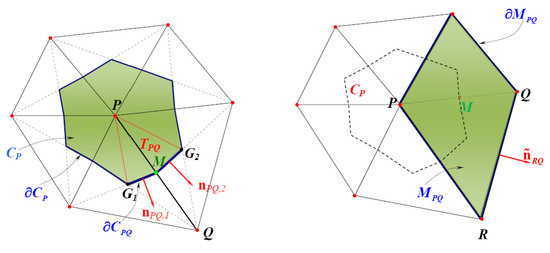
Figure 1. Median-dual computational cell implemented in the FV scheme (left) and the computational cell used for the gradient of the divergence in (2) (right).

3.1. The FV Approximation

After integration of (1) over each computational cell and application of the Gauss divergence theorem the semi-discrete form of the FV scheme reads as:

$$\frac{\partial {\mathbf{U}}_P}{\partial t}=-\frac{1}{\mid C_P\mid }\sum _{Q\in K_P}{\mathrm{\Phi }}_{PQ}-\frac{1}{\mid C_P\mid }{\mathrm{\Phi }}_{P,\mathrm{\Gamma }}+\frac{1}{\mid C_P\mid }{\int \int }_{C_P}\mathbf{S}d\mathrm{\Omega },$$

(9)

where ${\mathbf{U}}_P$ is the volume-averaged value of the conserved-liked quantities at a given time, $K_P$ is the set of the neighboring nodes to P, i.e., $K_P:=\{Q\in \mathbb{N}\mid \partial C_P\cap \partial C_Q\ne 0\}$, where $\mathrm{\Gamma }$ is the boundary of the computational domain $\mathrm{\Omega }$ and ${\mathrm{\Phi }}_{PQ},{\mathrm{\Phi }}_{P,\mathrm{\Gamma }}$ are the numerical flux vectors across each internal face, $\partial C_P$ and boundary face respectively.

The numerical fluxes are evaluated solving a Riemann problem at cell interfaces using the approximate Riemann solver of Roe [27]. To reach higher-order spatial accuracy an extension of the MUSCL methodology of Van Leer [28] is used. This extension relies on the evaluation of the fluxes with extrapolated physical variables $[h,u,v]$ at the midpoint M of an edge $PQ$. Each component of the physical variables and bed topography b are extrapolated using extrapolation gradients which are obtained using a combination of centered and upwind gradients [19,29,30,31] as to increase accuracy of the basic MUSCL reconstruction [30]. In this way a third-order spatial accuracy is obtained [19]. For the reduction of oscillations in cases where non-linearity prevails (e.g., when the dispersive terms become negligible) the use of a slope limiting procedure is necessary and the edge-based non-linear slope limiter of Van Albada–Van Leer is used. Details for the numerical model used such as wet/dry front treatment, boundary conditions and discretization of the dispersive terms can be found in [19,20].

3.2. The Resulting Linear System for the Velocity Field Recovery

Concerning the time discretization an optimal third order explicit Strong Stability Preserving Runge–Kutta (SSP-RK) method was adopted [19,32] under the usual CFL stability restriction. In each time step on the RK scheme the values of the velocities $u,v$ must be extracted from the new solution variable $\mathbf{P}={[P_1,P_2]}^T$ following from (2). The FV discretization of $\mathbf{P}$ results to a sparse matrix. The linear system $\mathbf{A}\mathbf{V}=\mathbf{C}$ with $\mathbf{A}\in {\mathbb{R}}^{2N\times 2N},\mathbf{V}={[{\mathbf{u}}_1{\mathbf{u}}_2\cdots {\mathbf{u}}_N]}^{\mathrm{T}}$ and $\mathbf{C}={[{\mathbf{P}}_1{\mathbf{P}}_2\cdots {\mathbf{P}}_N]}^{\mathrm{T}}$, has to be solved in each step of the RK time marching scheme.

Keeping in mind that $\mathbf{u}$ is our unknown velocity vector at each mesh node, each two rows of the matrix correspond to a node $P\in \{1,2,\dots N\}$ on the grid and for each such node we have,

$$H_P{\left[\frac{z_a^2}{2}\nabla (\nabla ·\mathbf{u})+z_a\nabla (\nabla ·h\mathbf{u})+\mathbf{u}\right]}_P={\mathbf{P}}_P.$$

(10)

Now the gradients $\nabla (\nabla ·\mathbf{u})$ and $\nabla (\nabla ·h\mathbf{u})$ must be computed. For that reason, we use the average of the gradient ${\left(\nabla w\right)}_P$ in a cell [33,34,35]:

$${\left(\nabla w\right)}_P=\frac{1}{\mid C_P\mid }\sum _{Q\in K_P}{w}_M{\mathbf{n}}_{PQ}.$$

(11)

which is computed in each mesh node P by applying the Green–Gauss theorem in the region ${\mathrm{\Omega }}_P$, i.e., the union of all triangles which share the vertex P and $w_M$ is the value of w at the midpoint of the edge $PQ$. The outward normal vector to $\partial C_{PQ}$ as ${\mathbf{n}}_{PQ}={[n_{PQx},n_{PQy}]}^{\mathrm{T}}$, while ${\tilde{\mathbf{n}}}_{PQ}$ is the corresponding unit vector. Using (11) Equation (10) reads as:

$$H_P\left[\frac{{\left(z_a^2\right)}_P}{2}\frac{1}{\mid C_P\mid }\sum _{Q\in K_P}{(\nabla ·\mathbf{u})}_M{\mathbf{n}}_{PQ}+\frac{{\left(z_a\right)}_P}{\mid C_P\mid }\sum _{Q\in K_P}{(\nabla ·h\mathbf{u})}_M{\mathbf{n}}_{PQ}+{\mathbf{u}}_P\right]={\mathbf{P}}_P,$$

(12)

and is now obvious that we have to compute $\nabla ·\mathbf{u}$ and $\nabla ·h\mathbf{u}$ at M. Referring again to Figure 1 (right panel), a new computational cell $M_{PQ}$ is defined, constructed by the union of two triangles which share the edge $PQ$. Hence, the discrete averages of the divergence can be computed as follows for $(\nabla ·\mathbf{u})$,

$${(\nabla ·\mathbf{u})}_M\approx \frac{1}{\mid M_{PQ}\mid }\sum _{\begin{array}{c}R,Q\in K_{PQ}\\ R\ne Q\end{array}}\frac{1}{2}\left({\mathbf{u}}_R+{\mathbf{u}}_Q\right)·{\mathbf{n}}_{RQ}$$

(13)

where $K_{PQ}=\{R\in \mathbb{N}\mid R\mathrm{is} \mathrm{a} \mathrm{vertex} \mathrm{of} M_{PQ} \mathrm{and} RQ\in \partial M_{PQ}.\}$ A similar computation is performed for the approximation of $(\nabla ·h\mathbf{u})$. We refer to [19] for more details on the discretization. By performing the above approximations we restrict the unknown information used in (10), i.e., values of $\mathbf{u}$, only to that coming from the nodes that are neighbors of node P, i.e., nodes $Q\in K_P$.

Substituting the above equation to (12) and for each node $P=1,\dots ,N$, gives:

$$\begin{array}{c}\hfill \frac{{\left(z_a^2\right)}_P}{2}\frac{H_P}{\mid C_P\mid }\sum _{Q\in K_P}\left[\frac{1}{\mid M_{PQ}\mid }\sum _{\begin{array}{c}R,Q\in K_{PQ}\\ R\ne Q\end{array}}\frac{1}{2}\left({\mathbf{u}}_R+{\mathbf{u}}_Q\right)·{\mathbf{n}}_{RQ}\right]{\mathbf{n}}_{PQ}+\\ \hfill +\frac{{\left(z_a\right)}_P{H}_P}{\mid C_P\mid }\sum _{Q\in K_P}\left[\frac{1}{\mid M_{PQ}\mid }\sum _{\begin{array}{c}R,Q\in K_{PQ}\\ R\ne Q\end{array}}\frac{1}{2}\left(h_R{\mathbf{u}}_R+h_Q{\mathbf{u}}_Q\right)·{\mathbf{n}}_{RQ}\right]{\mathbf{n}}_{PQ}={\mathbf{P}}_P,\end{array}$$

(14)

which can be further rewritten as:

$$\begin{array}{c}\hfill {\displaystyle \frac{{\left(z_a^2\right)}_P}{2\mid C_P\mid }\sum _{Q\in K_P}\left[\frac{1}{2\mid M_{PQ}\mid }\left(\sum _{\begin{array}{c}R,Q\in K_P\cap K_{PQ}\\ R\ne Q\end{array}}{\mathbf{u}}_R·\left({\mathbf{n}}_{PR}+{\mathbf{n}}_{RQ}\right)+{\mathbf{u}}_P·\left({\mathbf{n}}_{SP}+{\mathbf{n}}_{PR}\right)\right)\right]{\mathbf{n}}_{PQ}+}\\ \hfill {\displaystyle +\frac{{\left(z_a\right)}_P}{\mid C_P\mid }\sum _{Q\in K_P}\left[\frac{1}{2\mid M_{PQ}\mid }\left(\sum _{\begin{array}{c}R,Q\in K_P\cap K_{PQ}\\ R\ne Q\end{array}}{h}_R{\mathbf{u}}_R·\left({\mathbf{n}}_{PR}+{\mathbf{n}}_{RQ}\right)+h_P{\mathbf{u}}_P·\left({\mathbf{n}}_{SP}+{\mathbf{n}}_{PR}\right)\right)\right]{\mathbf{n}}_{PQ}=\frac{1}{H_P}{\mathbf{P}}_P.}\end{array}$$

(15)

After some calculations the resulting sparse $2N\times 2N$ linear system to be solved can be presented in a more compact form, as:

$$\frac{{\left(z_a^2\right)}_P}{2\mid C_P\mid }\sum _{Q\in K_P}\left({\mathbf{A}}_Q{\mathbf{u}}_Q+{\mathbf{A}}_P{\mathbf{u}}_P\right)+\frac{{\left(z_a\right)}_P}{\mid C_P\mid }\sum _{Q\in K_P}\left({\mathbf{B}}_Q{\mathbf{u}}_Q+{\mathbf{B}}_P{\mathbf{u}}_P\right)+{\mathbf{I}}_{\mathbf{2}}{\mathbf{u}}_P=\frac{1}{H_P}{\mathbf{P}}_P,P=1\dots N,$$

(16)

where the sub-matrices ${\mathbf{A}}_Q,{\mathbf{A}}_P,{\mathbf{B}}_Q$ and ${\mathbf{B}}_P$ now depend only on geometric quantities and the area $\mid M_{PQ}\mid$, and are given as

$${\mathbf{A}}_Q=\frac{1}{2\mid M_{PQ}\mid }\left[\begin{array}{cc}{\displaystyle \sum _{R,Q\in K_P\cap K_{PQ}}\left(n_{PRx}+n_{RQx}\right)n_{P{Q}_x}}& {\displaystyle \sum _{R,Q\in K_P\cap K_{PQ}}\left(n_{PRy}+n_{RQy}\right)n_{P{Q}_x}}\\ {\displaystyle \sum _{R,Q\in K_P\cap K_{PQ}}\left(n_{PRx}+n_{RQx}\right)n_{P{Q}_y}}& {\displaystyle \sum _{R,Q\in K_P\cap K_{PQ}}\left(n_{PRy}+n_{RQy}\right)n_{PQy}}\end{array}\right],$$

$${\mathbf{B}}_Q=\frac{1}{2\mid M_{PQ}\mid }\left[\begin{array}{cc}{\displaystyle \sum _{R,Q\in K_P\cap K_{PQ}}{h}_R\left(n_{PRx}+n_{RQx}\right)n_{P{Q}_x}}& {\displaystyle \sum _{R,Q\in K_P\cap K_{PQ}}{h}_R\left(n_{PRy}+n_{RQy}\right)n_{P{Q}_x}}\\ {\displaystyle \sum _{R,Q\in K_P\cap K_{PQ}}{h}_R\left(n_{PRx}+n_{RQx}\right)n_{P{Q}_y}}& {\displaystyle \sum _{R,Q\in K_P\cap K_{PQ}}{h}_R\left(n_{PRy}+n_{RQy}\right)n_{PQy}}\end{array}\right],$$

$${\mathbf{A}}_P=\frac{1}{2\mid M_{PQ}\mid }\left[\begin{array}{cc}\left(n_{SPx}+n_{PRx}\right)n_{P{Q}_x}& \left(n_{SPy}+n_{PRy}\right)n_{P{Q}_x}\\ \left(n_{SPx}+n_{PRx}\right)n_{P{Q}_y}& \left(n_{SPy}+n_{PRy}\right)n_{P{Q}_y}\end{array}\right]\mathrm{and}{\mathbf{B}}_P=h_P{\mathbf{A}}_{\mathbf{P}}.$$

The number of geometrical entries in each summation is always two, while the number of entries in the summation ${\displaystyle \sum _{Q\in K_P}}$ in (16) is equal to the number of the neighbors of P. This means that the maximum non-zero elements of the matrix in each row P in (16) are two times the number of the neighbors of node P plus one.

It is important to state here that, for the linear system (16) its coefficient matrix is constant in time. So it is constructed and stored, in a compressed sparse row CSR format [24], at a pre-processing stage at the beginning of each simulation. The present work concerns the solution process after the sparse matrix has been stored.

3.3. System’s Matrix Properties

The resulting system’s coefficient matrix is an un-symmetric but structurally symmetric matrix, in terms of its non-zero entries. It is often ill-conditioned and also mesh dependent. This means that the sparsity pattern of the matrix depends on the ordering of the nodes on each grid. Different grids lead to different matrix structures. In this work four type of grids are used, see Figure 2.

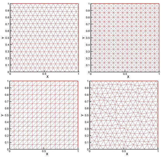
Figure 2. Representative grid types: Equilateral, Orthogonal I, Orthogonal II, Distorted (left to right).

For a given computational domain, and with out loss of generality, with dimensions $L_x\times L_y$ in the x- and y-direction respectively, we define a subdivision of $L_x$ by $N_x$ line segments, namely $D_x=L_x/N_x$ and depending on the grid type the corresponding subdivision $D_y$ of $L_y$ can be easily determined. As such, we define the characteristic length (effective mesh size) for each grid as ${\displaystyle h_N=\sqrt{\frac{L_x\times L_y}{N}}}$.

Figure 3 shows the structure of each matrix using the corresponding grids of Figure 2.

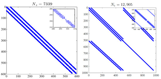
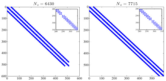
Figure 3. Matrix sparsity patterns for the four different mesh types shown in Figure 2 for $N_x=15$ with $N_z$ the number of non-zero elements.

Each grid used has 15 nodes in the x-axis ($N_x=15$) and the resulting matrix has $N_z$ non-zero elements shown. The resulting structure using the Orthogonal I type of grid is quite different from that of the other types which have a much smaller bandwidth. Further, for the Orthogonal I grid type the number of the non-zero elements, $N_z$, in the system’s matrix is almost double of that obtained from the other grids. Matrix structure remains the same while refining the meshes. Table 1 shows the characteristics of indicative matrices produced using for $L_x=L_y=1$ and different nodes in x-axis ($N_x$) while Table 2 show the $h_N$ values for each matrix reported in Table 1.

Table 1. Total ($2N\times 2N$) and non-zero elements ($N_z$) for the matrices produced for $L_x=Ly=1$ m with different $N_x$.

${\mathit{N}}_{\mathit{x}}$	Equilateral	Orthogonal I	Orthogonal II	Distorted
15	352,836 (7339)	925,444 (12,905)	262,144 (6430)	352,836 (7715)
30	4,857,616 (28,436)	13,853,284 (50,806)	3,694,084 (25,163)	4,857,616 (29,746)
60	7,4132,100 (118,293)	214,388,164 (201,931)	55,383,364 (99,258)	74,132,100 (118,293)

Table 2. The $h_N$ values for the matrices produced for $L_x=L_y=1$ m with different $N_x$.

${\mathit{N}}_{\mathit{x}}$	Equilateral	Orthogonal I	Orthogonal II	Distorted
15	0.058	0.0456	0.0625	0.058
30	0.0301	0.0232	0.0323	0.0301
60	0.0152	0.017	0.0164	0.0152

The properties of the matrix are also affected by the physical situation of the problem examined. The most important parameters are the still water level, h, see Equation (15), with relation to the nodes used on the grid, i.e., the resulting value of $h_N$. To illustrate the dependence on the ratio ${\displaystyle \frac{h}{h_N}}$ the spectrum of eigenvalues for six matrices are shown in Figure 4 and Figure 5. The six matrices examined have been produced using two type of grids, equilateral and Orthogonal I. Figure 4 shows the eigenvalues of three matrices produced using the equilateral type of grid. The first matrix (on the left) has $h=1$ m and $h_N=0.058$ the second (center) uses $h=1$ m$,h_N=0.0301$ and the third one (right) uses $h=100$ m and $h_N=0.058$. All matrices have minimum eigenvalues near zero and it is noted that as the ratio ${\displaystyle \frac{h}{h_N}}$ grows the spectrum of the matrix has a much larger spread of eigenvalues through the right half of the complex plane. The same conclusions can be obtained from Figure 5 which depicts the spectrum of eigenvalues for three matrices, obtained using the Orthogonal I type of grid. The parameters used are the same as in Figure 4.

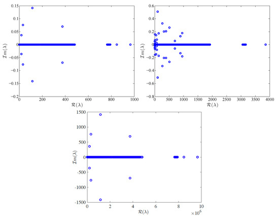
Figure 4. Eigenvalues of three matrices using the equilateral type of grid with $\frac{h}{h_N}=\frac{1}{0.058}$ (top left), $\frac{1}{0.031}$ (top right) and $\frac{100}{0.058}$ (bottom).

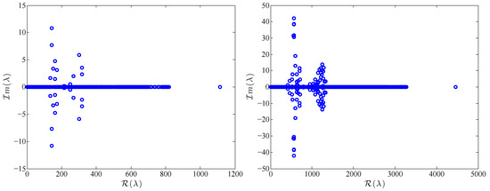
Figure 5. Eigenvalues of three matrices using the Orthogonal I type of grid with $\frac{h}{h_N}=\frac{1}{0.0456}$ (top left), $\frac{1}{0.0232}$ (top right) and $\frac{100}{0.0456}$ (bottom).

The above behavior gives evidence that preconditioning is crucial in this type of problems. These conclusions are further reflected in the respective condition numbers of the three matrices which are between $O\left({10}^3\right)$–$O\left({10}^5\right)$. For example the matrix produced by the distorted grid and $h=1$ m,$N_x=15$ (see Figure 2) has a condition number equal to $7.7732\times {10}^5$ while the one produced from the equilateral grid has condition number $5.5348\times {10}^3$. The matrices become even more ill-conditioned as the depth is further increased, or the grid is refined. Similar behavior has been mentioned in [10] where the finite difference method is used to solve a Boussinesq model in two dimensions.

4. Iterative Methods, Preconditioning and Reordering

4.1. Application of Iterative Methods

In this presentation, we want to develop an optimal strategy for the solution of system (16) abbreviated to Ax = b, and we use a “toy” problem in which the right hand side vector $\mathbf{b}$ is computed adding the columns of the matrix $\mathbf{A}$. The initial guess used for the iterative methods discussed next was the zero vector. From now on all test cases presented will solve this “toy” problem unless otherwise stated. We mention again here that the system’s matrix depends on the numbering and the geometrical quantities of the mesh nodes. So, and since it is not depending on the unknown quantities of the BT model we can construct it and store it only once in the beginning of our simulation.

One common solution method for sparse systems $\mathbf{Ax}=\mathbf{b}$ is to use a sparse direct solution algorithm via a complete factorization of the matrix. However, for large scale problems concluding to large sparse linear systems, the computational time required for the factorization along with the storage requirements can be an insurmountable problem [36]. An alternative to direct solution methods is the use of iterative ones, which have significantly lower storage demands. Two classical Krylov Subspace iterative methods are used in this work. The Generalized Minimal Residual (GMRES) and the Biconjucate Gradient Stabilized (BiCGStab) algorithms. Both methods are implemented using the SPARSKIT package [26]. The optimal solution strategy depends on factors such as problem size, sparsity pattern and the matrix’s eigenspectrum. We note here that, during the course of this work several other iterative methods such the Flexible version of Generalized Minimal Residual Method (FGMRES), the Quasi Minimum Residual Method (QMR) and the Transpose Free QMR (TFQMR) where considered. However, the GMRES and the BiCGStab methods where proven more robust in solving the problem at hand and for brevity we present the efficient application and obtained results for these two.

Figure 6 depicts the performance (in terms of CPU time) of each method for two different type of grids, of the Equilateral type (left) and the Orthogonal I type. Each sub-figure depict the computational time needed as to solve the sparse system while the nodes are refined and the depth is increased.

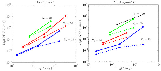
Figure 6. CPU time versus variable still water level to $h_N$ ratio for GMRES (solid line) and BiCGStab (dashed line).

For both cases we can see that the computational time grows dramatically not only as the mesh is refined (which is expected) but also as the still water level h (with respect to $h_N$) is increased. Furthermore, comparing the CPU times needed for each iterative method we can see that they start to vary as the water depth to $h_N$ ratio is increased. The BiCGStab method solves the linear systems produced (for both types of grid) in less time than the GMRES. In some cases both methods could not reach convergence for higher $h/h_N$ values. This was more prominent for GMRES. For both iterative methods a relative residual error tolerance $r={\parallel b-Ax\parallel }_2/{\parallel b\parallel }_2\le {10}^{-6}$ was used as the convergence criterion. Following from the above, we can clearly understand that the usage of a preconditioning method is mandatory as to reduce the number of iterations needed and consequently the total computational time.

4.2. Application of Preconditioning Methods

Although Krylov Subspace iterative methods are well suited to solve relatively sparse system, they can exhibit slow convergence. Thus, it is essential to use a good preconditioning strategy as to enhance their convergence properties and reduce the computational cost. A survey of preconditioning techniques for large linear systems can be found in [25,37]. To this end, this section introduces the different techniques of preconditioning tested.

A good preconditioner must approximates matrix $\mathbf{A}$ well, while at the same time being easy to solve. Let $\mathbf{M}$ be a new non-singular matrix which is a good approximation of $\mathbf{A}$. The preconditioned system ${\mathbf{M}}^{-\mathbf{1}}\mathbf{A}\mathbf{x}={\mathbf{M}}^{-\mathbf{1}}\mathbf{b}$ will have the same solution as system $\mathbf{A}\mathbf{x}=\mathbf{b}$, and it can be solved easier. The non-singular matrix $\mathbf{M}$ is called preconditioner. In the present work all preconditioning is done from the left even though preconditioning from the right has been found to be equally effective. Three preconditioning techniques, which are freely available as part of the SPARSKIT [26] package, were implemented and tested; the ILU(0), ILU(k) and ILUT preconditioners.

Since convergence of an iterative method, such as the GMRES and BiCGStab, depends on the eigenvalues of the matrix, generally speaking, preconditioning attempts to improve the spectral properties of $\mathbf{A}$ [25]. A “good” preconditioner transforms the matrix so that the original sparse linear system can be solved easily, with low storage demands, at low computational expense. The preconditioned matrix should have eigenvalues away from zero. Even for non-symmetric matrices with a cluster of the eigenvalue spectrum away from zero can still lead to a rapid convergence.

One way to approach this is to use a direct method such as $\mathbf{LU}$-decomposition, i.e., $\mathbf{M}=\mathbf{LU}$. The system can then be solved in two steps using the factors $\mathbf{L}$ and $\mathbf{U}$. The drawback of this method is that during the factorization process, matrices $\mathbf{L}$ and $\mathbf{U}$ are dense so the computer storage demands and the dimension of the problem may become huge. One of the simplest ways of defining a preconditioner is to perform an incomplete factorization of the original matrix A. This entails a decomposition of the form $\mathbf{A}=\mathbf{LU}-\mathbf{R}$ where L and U have the same nonzero structure as the lower and the upper part of A, respectively and R is the residual matrix of the factorization. This incomplete factorization is known as ILU(0) and often leads to a crude approximation which in turn may result to the need of many iterations to reach converge. To remedy this, several alternative incomplete factorizations have been developed by allowing more fill-ins in L and U. In practice, and as to find the L and U, the Gaussian elimination process is used and a level of fill-in is attributed to each element which is dropped or not according to this value [24]. In general, a more accurate ILU factorization requires fewer iterations to converge but of course the preprocessing cost to compute the factors is higher. Incomplete factorizations that rely on the level of fill are blind to numerical values because elements that are dropped depend only on the structure of the matrix. Some methods are available based on dropping elements in the Gaussian elimination process according to their magnitude rather than their location.

Different factorization algorithms have different rules that govern the dropping or fill-in in the incomplete factors. In this work two rules were used; the level of fill approach and the use of a drop tolerance parameter. From now on applying a dropping rule to an element will only mean replacing the element with zero if it satisfies a set of criteria. The drop tolerance is a positive number $\tau$ which is used in a dropping criterion. The dropping strategy depends on the matrix, the non-zero numbers and the conditional number. The philosophy of that is to accept only the values greater (in absolute value) than the tolerance in the new fill-ins. In general, it is difficult to choose the right value for the drop tolerance, because one cannot predict the amount of storage that will be needed.

4.2.1. The ILU(0) Preconditioner

When the level of fill-in is equal to zero then the ILU(0) preconditioner in the ILU factorization is recovered. So, ILU(0) refers to a full factorization, with no reduction or fill-in, and it is also called the no-fill ILU preconditioner. We tested this preconditioner for systems produced for two types of grids, namely the Equilateral and Orthogonal of type I, using the two iterative methods (GMRES and BiCGStab). The computational values in the toy problem were $h=1$ m and $N_x=15,30,60,120.$ For the Equilateral type of grid none of the two iterative methods was able to converge while for the Orthogonal I type of grid only the BiCGStab method for $N_x=30$ converged after 34,957 iterations. Even though the ILU(0) preconditioner is easy to implement and its computation is inexpensive, it is effective mainly for simpler problems. By simpler problems we mean, for example, low-order discretizations of scalar elliptic PDEs leading to non-singular matrices and diagonally dominated matrices. These are the type of problems for which these preconditioners were originally proposed [25]. For this case study the non-fill factorization resulted in too crude approximation of the matrix $\mathbf{A}$, so more sophisticated preconditioners had to be used.

4.2.2. The ILU(k) Preconditioner

The computation of the ILU(k) preconditioner requires only the fill-in criterion. So, if k is a non-negative integer, all the fill-ins whose level is greater than k are dropped. The limitation of this process is that for matrices that are not diagonal dominated ILU(k) requires to store many fill-ins that are small in absolute value leading to expensive computations and in preconditioner of lower quality. In this work, we used the value $k=300$ elements per row (in the factors) which has been found to be a good universal parameter for the problems presented here.

Figure 7 demonstrates how the performance of the iterative methods is affected by the application of the ILU(k) strategy in terms of the increasing still water level to $h_N$ ratio for system matrices produced by Equilateral type of grids. The iterations needed for convergence vary between 2 and 4 for both methods. Comparing with Figure 6, a substantial improvement in computational time can be observed. The results show that the total time needed for convergences is not affected by the ratio $h/h_N$ but, as expected, is highly increased while increasing the number of unknowns of the problem (for larger $N_x$ values i.e., smaller $h_N$ values). The two iterative methods needed the same computational time.

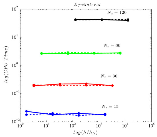
Figure 7. CPU time versus $h/h_N$ for GMRES (solid line) and BiCGStab (dashed line) using the ILU(k) preconditioner with $k=300$.

Table 3 presents the actual times and iterations needed for the solution of the linear systems produced using the Orthogonal I type of mesh. We must note here that, whenever the results are omitted or a dash is placed then the iterative method used failed to converge. It can be concluded from Table 3 that, as the ratio $h/h_N$ increases from a grid refinement, i.e., lower values of $h_N$ are produced, the computational time dramatically increases and in some cases convergence can not be obtained for system resulting from this type of grid. The main reasons for this are, the large amount of nodes in the mesh, compared to the other types of meshes (see Table 2) and the different coefficient matrix structure, which has a bigger bandwidth (please refer to Figure 3). For this grid type, and although its is a structured one, the ILU(k) preconditioner fails to improve the condition of the matrix for finer meshes even though the iterations needed for the converged are significantly decreased at coarser ones.

Table 3. CPU time for the solution of linear systems resulting from Orthogonal I type of grids using the ILU(k) preconditioner, with $k=300$, preconditioner.

$\mathit{h}/{\mathit{h}}_{\mathit{N}}$	GMRES (s)/Iterations	BiCGStab (s)/Iterations
0.1/0.0456	1.588515759/2	1.588515759/3
1.0/0.0456	1.525697947/2	1.581536055/3
10/0.0456	1.580311775/3	1.591470003/3
0.1/0.0232	87.64499593/2	87.37235212/3
10/0.0232	-	87.47821903/3

It should be noted here that, the total time needed for the computation of the preconditioner is independent of the still water depth h. The actual CPU times needed are for matrices resulting from refined meshes for the two grid types are presented in Table 4. These times are very small compared to the total time needed for the iterative methods to reach convergence.

Table 4. Times needed for the ILU(k) preconditioner’s computation.

${\mathit{N}}_{\mathit{x}}$	Equilateral (s)	Orthogonal I (s)
15	0.014	0.012
30	0.19	0.15
60	2.62	2.24
120	-	-

4.2.3. ILUT($p,\tau$) Preconditioner:

The general algorithm of preconditioner ILU with threshold, ILUT($p,\tau$), includes a set of rules for dropping small elements. Thus, the use of ILUT produces a lower storage factorization. The main idea here is to replace an element with zero if its value is smaller than a threshold value $\tau$, set by the user. The dropping rule can be applied to a row, by checking all the elements and keeping/ignoring them depending on their arithmetic value [24]. By increasing the drop tolerance (threshold) the sparsity of the preconditioner increases and the amount of work that will be needed for applying the preconditioner decreases. The limitation here is that the application of the ILUT can affect the solution’s accuracy thus, the iterative methods may require more iterations to converge. An additional dropping rule which can be applied is to keep only the p-th largest elements in the L part of the row and the p-th largest elements in the U part of the row in addition to the diagonal element, which is always kept. In this work we use always $p=300.$ The goal of this dropping step is to control the number of elements per row.

Figure 8 presents, like before, how the performance of the ILUT strategy is affected by the variable water depth to $h_N$ ratio, for the matrices produced by the equilateral type of grid. The threshold value used here was set to $\tau ={10}^{-5}$. The iterations needed for convergence varied for 3–13 but the CPU time needed is slightly less compered to the one obtained using the ILU(k) preconditioner (as presented in Figure 7) for higher $h/h_N$ values. For smaller ratios some time improvements can be noticed. We must acknowledge here that for the systems produced by the Orthogonal I type of grid both iterative methods failed to converge. Lowering the threshold value $\tau$ lead to no substantial improvement in computational efficiency or convergence of the iterative methods.

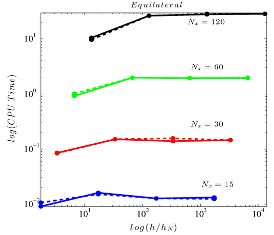
Figure 8. CPU time versus $h/h_N$ for GMRES (solid line) and BiCGStab (dashed line) applying the ILUT preconditioner with $\tau ={10}^{-5}$.

5. Reordering

Since all preconditioners applied in the previous section failed to substantially improve the condition of the produced matrices as to decrease the iterations for convergence and/or the computational time needed and in some cases no convergence could be obtained, we must use a reordering technique so as to improve the stability of the incomplete factorizations. It is well known that the incomplete factorization preconditioners are sensitive to the ordering of unknowns and equations [25]. Optimal reordering strategies can be used with the dual purpose of limiting the bandwidth of the discrete operator A and to reduce excessive fill-in in the factorization of the involved operators [38]. In most cases, reordering techniques tend to affect the rate of convergence of preconditioned Krylov subspace methods [25]. These algorithms aim to minimize the bandwidth of the matrix $\mathbf{A}$. Two different approaches were used in this work namely, the Cuthill–McKee (CMK) and the Reverse Cuthill–McKee (RCM) permutations.

Figure 9 shows the CPU time versus the relative water depth for two types of grids using again the GMRES and BiCGStab algorithms implementing the ILU(k) preconditioner with $k=300$ and with CMK reordering. As can be seen in Figure 9 the usage of CMK reordering in addition to the ILU(k) preconditioner slightly improves the convergence process, when compared to the single usage of the preconditioner in to Figure 7 for the equilateral type of grids. However, it can also be observed that on grids with the same degrees for freedom, increasing the water depth does not affect the computational time needed.

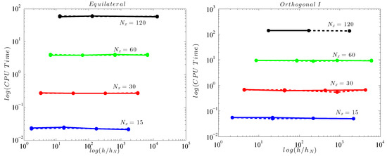
Figure 9. CPU time versus $h/h_N$ for GMRES (solid line) and BiCGStab (dashed line) using the ILU(k) preconditioner and CMK reordering.

Using the ILUT preconditioner and the CMK reordering (see Figure 10) the computational results vary. We tested different values of drop tolerance $\tau$ for this preconditioner. For values greater than ${10}^{-5}$ none of the iterative methods was able to converge. Figure 10 shows the CPU time versus the relative water depth using CMK and ILUT with drop tolerance ${10}^{-5}$ (left column). Even though we observe convergence to the solution for most of the test cases, the computational time increased as the relative water depth was increased. This makes the choice of the drop tolerance unsuitable for physical problems with relative large water depth. Using a smaller value for $\tau ={10}^{-10}$ (see Figure 10 right column) the behavior of the linear systems, especially when using GMRES, closely approximates the behavior shown in Figure 9 since the CPU time is not affected by the variation of the ratio $(h/h_N)$ (using the same degrees of freedom). The results of this work confirm also those found in [10], where non-linear and highly dispersive Boussinesq equations are solve using a finite difference scheme. The ILUT preconditioner works quite well in shallow to intermediate water depths, however may rapidly lose effectiveness as the depth is further increased. However, a big improvement was that, for systems produced from Orthogonal I type grids, in this case, both iterative methods converged with satisfactory performance.

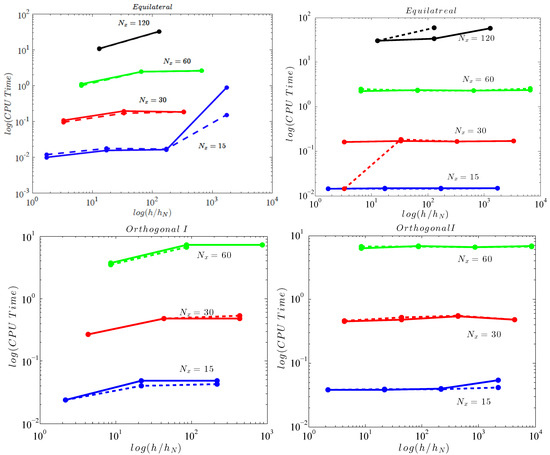
Figure 10. CPU time versus variable water depth for GMRES (solid line) and BiCGStab (dashed line) using ILUT preconditioner with threshold ${10}^{-5}$ (left) and ${10}^{-10}$ (right) and CMK reordering, for Equilateral type of grid (up) and for Orthogonal I (down).

One of the most common reordering techniques, used mostly with the finite element method, is the Reverse Cuthill–McKee (RCM) ordering [39]. The work of Benzi et al. [40], on ordering for incomplete factorization, revealed that the use of RCM method was advantageous for non-symmetric problems.

Figure 11 depicts the CPU time versus the ratio $h/h_N$ using the ILU(k) preconditioner and the RCM reordering while Figure 12 shows the same but with the usage of the ILUT preconditioner and the RCM reordering. Again two different tolerances have been used. The same behavior as the one presented in Figure 9 and Figure 10 can be observed.

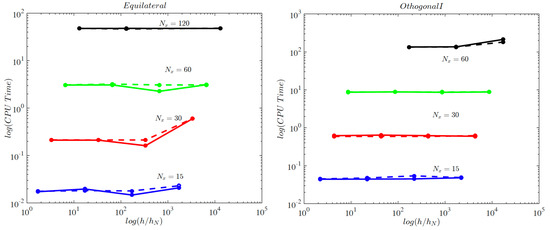
Figure 11. CPU time versus variable water depth for GMRES (solid line) and BiCGStab (dashed line) using ILU(k) preconditioner and RCM reordering, for Equilateral type of grids (left) and for Orthogonal I types (right).

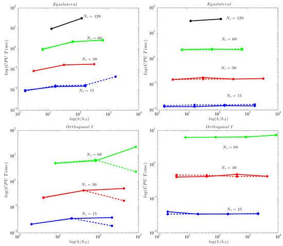
Figure 12. CPU time versus variable water depth for GMRES (solid line) and BiCGStab (dashed line) using ILUT preconditioner with threshold ${10}^{-5}$ (left) and ${10}^{-10}$ (right) and RCM reordering for Equilateral type of grids (up) and Orthogonal I types (down).

Spatial Accuracy and Efficiency

We performed studies for the accuracy and efficiency of the FV numerical from [19] considering the propagation of a solitary wave over an undisturbed depth using distorted grids. The numerical test case consists of a solitary wave of amplitude $A=0.1$ m which propagates over a flat topography of depth $h=1$ m. The computational domain was $(x,y)\in$ [$0,300$ m] × [$0,5$ m]. To prove the validity of the current study we examined the total and per time- step CPU time need to advance the model in one time-step and additionally the total and per time-step CPU times for the solutions of the $2N\times 2N$ sparse linear system, using the BiCGStab method.

As shown in Figure 13 the CPU time grows like $O\left(\right|\left|E\left(\eta \right)\right|{|}^{-1})$ (linearly) while the time needed by the BiCGStab (as to solve the linear system) like $O\left(\right|\left|E\left(\eta \right)\right|{|}^{-0.85})$, for the finer grids, where $\left|\right|E\left(\eta \right)\left|\right|$ is the error of the free surface elevation, $\eta$, measured in $L_2$ norm. However, and due to the increase of the number of time steps needed on finer grids, the total CPU time grows approximately like $O\left(\right|\left|E\left(\eta \right)\right|{|}^{-1.25})$ while the total time needed by the BiCGStab like $O\left(\right|\left|E\left(\eta \right)\right|{|}^{-1.5})$ and starts to dominate the overall time, as grids become refined.

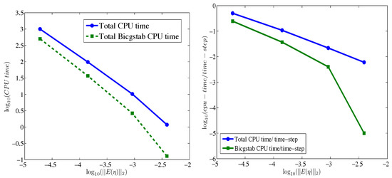
Figure 13. CPU times as a function of the free surface error measured in the $L_2$ norm.

To assess the effect that the increase of the number of grid points N has to the storage requirements of the non-zero elements ($N_z$) of the $2N\times 2N$ sparse linear system and to the computational efficiency, we present relevant comparison in Figure 14. As expected, the $N_z$ entries grow almost linearly with respect to N. The BiCGStab CPU time per time step scales like $O\left(N^{3/2}\right)$ however, the total CPU time per time step is growing like $O\left(N^{5/4}\right)$, close to linear.

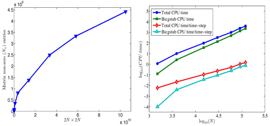
Figure 14. Non-zero elements as a function of N (left) and CPU times as a function of N (right).

All computations were performed on a shared memory machine HP DL180G6 (HP, Palo Alto, CA, USA) consists of two 6-core Xeon X5660@2.8GHz type processor with 12 MB Level 3 cache memory. The total memory is 64 GB and the operating system is Oracle Linux version 6.1. The application is developed in double precision Fortran code using Oracle Solaris Studio compilers version 12.2.

6. Conclusions

In this work, we have attempted to highlight the importance of utilizing two well-known iterative methods along with preconditioning and reordering methods for the ill-conditioned sparce linear systems that arise from the numerical integration of the of the extended Boussinesq-type equations that model dispersive wave propagation. To this end, a numerical study is presented for solving these sparse linear systems that results from a finite volume discretization of the extended Boussinesq-type equations of Nwogu on unstructured triangular 2D meshes. The linear system arises due to the reformulation of the model’s equations in conservative-like form and its solution is essential to recover the actual velocity field in the flow. The resulting system’s coefficient matrices are structurally symmetric and sparse but in most cases ill-conditioned. The system’s numerical solution consumes much of the actual computation time needed for the numerical scheme to advance one discrete time step, especially as the meshes become finer. The effect of the grids resolution along with the physical value of the still water reference in the problem was investigated. Different iterative methods, precondition and reordering techniques were investigated as to to conclude to a an optimal and robust strategy for the system’s solution. For the resulting system, its coefficient matrix is constant in time. So it is constructed and stored, in a compressed sparse row CSR format, at a pre-processing stage at the beginning of each simulation. The present work concerns the solution process after the sparse matrix has been stored. Then it is reordered and the preconditioner of the reordered matrix is computed at this pre-processing stage and subsequently utilized to solve the linear system at each time step. The following major conclusions can be drawn from this work:

• BiCGSTAB and GMRES iterative methods give almost similar results for the resulting systems, with the BiCGSTAB to have been proven more robust in some cases and is the method of choice following from this work.
• The usage of preconditioning and/or reordering is mandatory as to achieve convergence for the different mesh types used.
• Using preconditioning and reordering we gained convergence for (all) systems in every water depth. Using only preconditioning we were able to solve efficiently systems that have a small condition number (usually derived from equilateral grids).
• Using a drop tolerance $\tau ={10}^{-5}$ (for ILU(k) and ILUT preconditioners): CPU time using ILUT is less than that of using ILU(k) in average water depths. The usage of ILU(k) maybe more expensive in time but results on an overall the same CPU time in any water depth for the same grid resolution for convergence.
• As to correct the limitation of ILUT we decreased the drop tolerance and we observed that for larger water depths both iterative methods converge, but of course with an additional time cost. Like before the CPU time is independent on the relative water depth on each matrix.
• The Reverse Cuthill–McKee (RCM) ordering was proven more efficient compared to the Cuthill–McKee (CMK) ordering. This is found to greatly improve the efficiency of the ILUT preconditioner, since it constrains the factorized matrix to lie within a much narrower bandwidth and hence the incomplete factorization is generally more accurate for a prespecified amount of storage.

References

- Peregrine, D.H. Long waves on a beach. J. Fluid Mech. 1967, 27, 815–882. [Google Scholar] [CrossRef]
- Madsen, P.; Sørensen, O.R.; Schäffer, H.A. Surf zone dynamics simulated by a Boussinesq-type model: Part I. Model description and cross-shore motion of regular waves. Coast. Eng. 1997, 32, 255–288. [Google Scholar] [CrossRef]
- Nwogu, O. An alternative form of the Boussinesq equations for nearshore wave propagation. J. Waterw. Port Coastal Ocean Eng. 1994, 119, 618–638. [Google Scholar] [CrossRef]
- Madsen, P.A.; Sørensen, O.R. A new form of the Boussinesq equations with improved linear dispersion characteristics. Part 2: A slowing varying bathymetry. Coast. Eng. 1992, 18, 183–204. [Google Scholar] [CrossRef]
- Gobbi, M.F.; Kirby, J.T.; Wei, G. A fully non-linear Boussinesq model for surface waves. Part 2. Extension to O(kh4). J. Fluid Mech. 2000, 405, 181. [Google Scholar] [CrossRef]
- Lynett, P.; Liu, P.L.F. A two-layer approach to wave modeling. Proc. R. Soc. Lond. Ser. 2004, 460, 2637–2669. [Google Scholar] [CrossRef]
- Tissier, M.; Bonneton, P.; Marche, F.; Chazel, F.; Lannes, D. A new approach to handle wave breaking in fully non-linear Boussinesq models. Coast. Eng. 2012, 67, 54–66. [Google Scholar] [CrossRef]
- Wei, G.; Kirby, J.T. A time-dependent numerical code for extended Boussinesq equations. J. Waterw. Port Coastal Ocsean Eng. 1995, 120, 251–261. [Google Scholar] [CrossRef]
- Brocchini, M. A reasoned overview on Boussinesq-type models: The interplay between physics, mathematics and numerics. Proc. R. Soc. A 2013, 469. [Google Scholar] [CrossRef]
- Fuhrman, D.R.; Madsen, P.A. Simulation of nonlinear wave run-up with a high-order Boussinesq model. Coast. Eng. 2008, 55, 139–154. [Google Scholar] [CrossRef]
- Eskilsson, C.; Sherwin, S.J. Spectral/hp discontinuous Galerkin methods for modelling 2D Boussinesq equations. J. Comp. Phys. 2006, 210, 566. [Google Scholar] [CrossRef]
- Walkey, M.; Berzins, M. A finite element method for the two-dimensional extended Boussinesq equations. Int. J. Numer. Meth. Fluids 2002, 39, 865. [Google Scholar] [CrossRef]
- Ricchiuto, M.; Filippini, A.G. Upwind residual discretization of enhanced Boussinesq equations. J. Comp. Phys. 2014, 271, 306–341. [Google Scholar] [CrossRef]
- Erduran, K.S. Further application of hybrid solution to another form of Boussinesq equations and comparisons. Int. J. Numer. Methods Fluids 2007, 53, 827–849. [Google Scholar] [CrossRef]
- El Asmar, W.; Nwogu, O. Finite volume solution of Boussinesq-type equations on an unstructured grid. In Proceedings of the 30th International Conference on Coastal Engineering, San Diego, CA, USA, 3–8 September 2006; McKee Smith, J., Ed.; World Scientific: Singapore, 2006; pp. 73–85. [Google Scholar]
- Shi, F.; Kirby, J.T.; Harris, J.C.; Geiman, J.D.; Grilli, S.T. A high-order adaptive time-stepping TVD solver for Boussinesq modeling of breaking waves and coastal inundation. Ocean Model. 2012, 43–44, 36–51. [Google Scholar] [CrossRef]
- Roeber, V.; Cheung, K.F.; Kobayashi, M.H. Shock-capturing Boussinesq-type model for nearshore wave processes. Coast. Eng. 2010, 57, 407–423. [Google Scholar] [CrossRef]
- Tonelli, M.; Petti, M. Hybrid finite-volume finite-difference scheme for 2DH improved Boussinesq equations. Coast. Eng. 2009, 56, 609–620. [Google Scholar] [CrossRef]
- Kazolea, M.; Delis, A.I.; Nikolos, I.A.; Synolakis, C.E. An unstructured finite volume numerical scheme for extended 2D Boussinesq-type equations. Coast. Eng. 2012, 69, 42–66. [Google Scholar] [CrossRef]
- Kazolea, M.; Delis, A.I.; Synolakis, C.E. Numerical treatment of wave breaking on unstructured finite volume approximations for extended Boussinesq-type equations. J. Comp. Phys. 2014, 271, 281–305. [Google Scholar] [CrossRef]
- Zhang, S.; Zhu, L.; Li, J. Numerical Simulation of Wave Propagation, Breaking, and Setup on Steep Fringing Reefs. Water 2018, 10, 1147. [Google Scholar] [CrossRef]
- Liu, W.; Ning, Y.; Zhang, Y.; Zhang, J. Shock-Capturing Boussinesq Modelling of Broken Wave Characteristics Near a Vertical Seawall. Water 2018, 10, 1876. [Google Scholar] [CrossRef]
- Kazolea, M.; Delis, A. Irregular wave propagation with a 2DH Boussinesq-type model and an unstructured finite volume scheme. Eur. J. Mech. B/Fluids 2018, 72, 432–448. [Google Scholar] [CrossRef]
- Saad, Y. Iterative Methods for Sparse Linear Systems; SIAM: Philadelphia, PA, USA, 2003. [Google Scholar]
- Benzi, M. Preconditioning Techniques for Large Linear Systems: A Survey. J. Comp. Phys. 2002, 182, 418–477. [Google Scholar] [CrossRef]
- Saad, Y. SPARSKIT: A Basic Tool Kit for Sparse Matrix Computations, Version 2. Available online: https://people.sc.fsu.edu/~jburkardt/f77_src/sparsekit/sparsekit.html (accessed on 20 January 2021).
- Roe, P.L. Approximate Riemann Solvers, Parameter Vectors, and Difference Schemes. J. Comp. Phys. 1981, 43, 357–372. [Google Scholar] [CrossRef]
- van Leer, B. Towards the ultimate conservative difference scheme V. A second order sequel to Godunov’s method. J. Comp. Phys. 1979, 32, 101. [Google Scholar] [CrossRef]
- Barth, T.J. A 3-D Upwind Euler Solver for Unstructured Meshes; AIAA Paper 91-1548CP; AIAA: Reston, VA, USA, 1991. [Google Scholar]
- Delis, A.I.; Nikolos, I.K.; Kazolea, M. Performance and comparison of cell-centered and node-centered unstructured finite volume discretizations for shallow water free surface flows. Arch. Comput. Methods Eng. 2011, 18, 57–118. [Google Scholar] [CrossRef]
- Smith, T.M.; Barone, M.F.; Bond, R.B. Comparison of reconstruction techniques for unstructured mesh vertex centered finite volume schemes. In Proceedings of the 18th AIAA Computational Fluid Dynamics Conference, Miami, FL, USA, 25– 28 June 2007; pp. 1–22. [Google Scholar]
- Spiteri, R.J.; Ruuth, S.J. A new class of optimal high-order strong-stability-preserving time discretization methods. SIAM J. Numer. Anal. 2002, 40, 469. [Google Scholar] [CrossRef]
- Barth, T.J. Aspects of Unstructured grids and finite volume solvers for the Euler and NAvier-Stokes equations. In Special Course on Unstructured Grid Methods for Advection Dominated Flows; AGARD Report; NATO: Paris, France, 1992; Volume 787. [Google Scholar]
- Barth, T.J. Numerical Methods and Error Estimation for Conservation laws on Structured and Unstructured Meshes; VKI Computational Fluid Dynamics Lecture Series; VKI: Waterloosesteenweg, Belgium, 2003. [Google Scholar]
- Barth, T.J.; Ohlberger, M. Finite volume methods: Foundation and analysis. In Encyclopedia of Computational Mechanics; Stein, E., de Borst, R., Hudges, T., Eds.; John Wiley and Sons Ltd.: Hoboken, NJ, USA, 2004. [Google Scholar]
- Olshanskii, M.; Tyrtyshnikon, E. Iterative Methods for Linear Systems; SIAM: Philadelphia, PA, USA, 2015. [Google Scholar]
- Wathen, A. Preconditioning. Acta Numer. 2015, 24, 329–376. [Google Scholar] [CrossRef]
- Engsig-Karup, A.P. Unstructured Nodal DG-FEM Solution of High-Order Boussinesq-Type Equations. Ph.D. Thesis, Technical University of Denmark, Kongens Lyngby, Denmark, 2006. [Google Scholar]
- George, A.; Liu, J.W.H. Computer Solution of Large Sparce Positive Definite Systems; Prentice Hall: Englewood Cliffs, NJ, USA, 1981. [Google Scholar]
- Benzi, M.; Szyld, D.B.; Duin, A.V. Orderings for incomplete factorization preconditioning of nonsymmetric problems. SIAM J. Sci. Comput. 1999, 20, 1652–1670. [Google Scholar] [CrossRef]
Publisher’s Note: MDPI stays neutral with regard to jurisdictional claims in published maps and institutional affiliations. |
© 2022 by the authors. Licensee MDPI, Basel, Switzerland. This article is an open access article distributed under the terms and conditions of the Creative Commons Attribution (CC BY) license (https://creativecommons.org/licenses/by/4.0/).