


Flood Risk Assessment of Buildings Based on Vulnerability Curve: A Case Study in Anji County

 ,
,
Abstract
1. Introduction
2. Study Area and Data
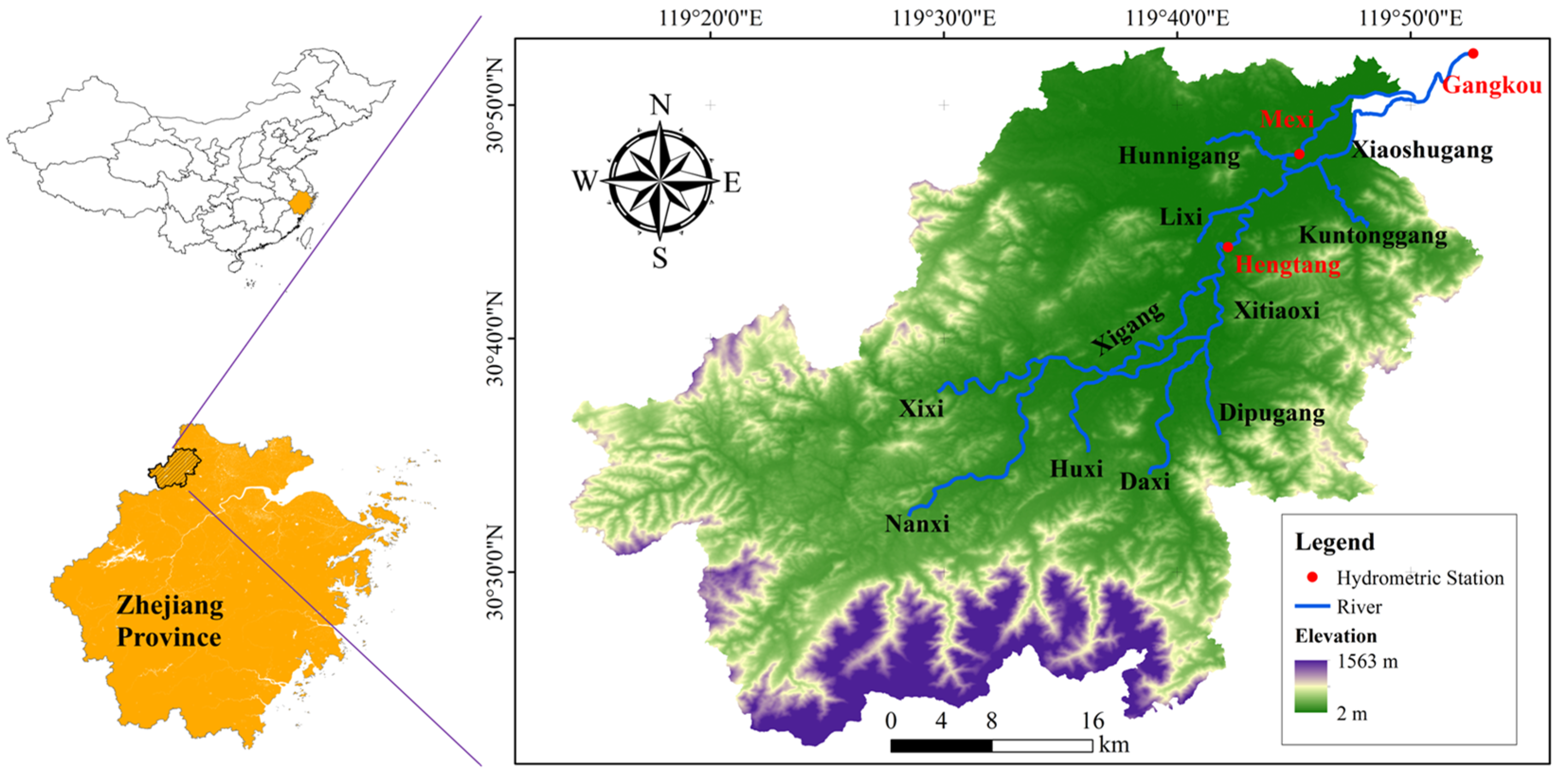
2.1. Anji County
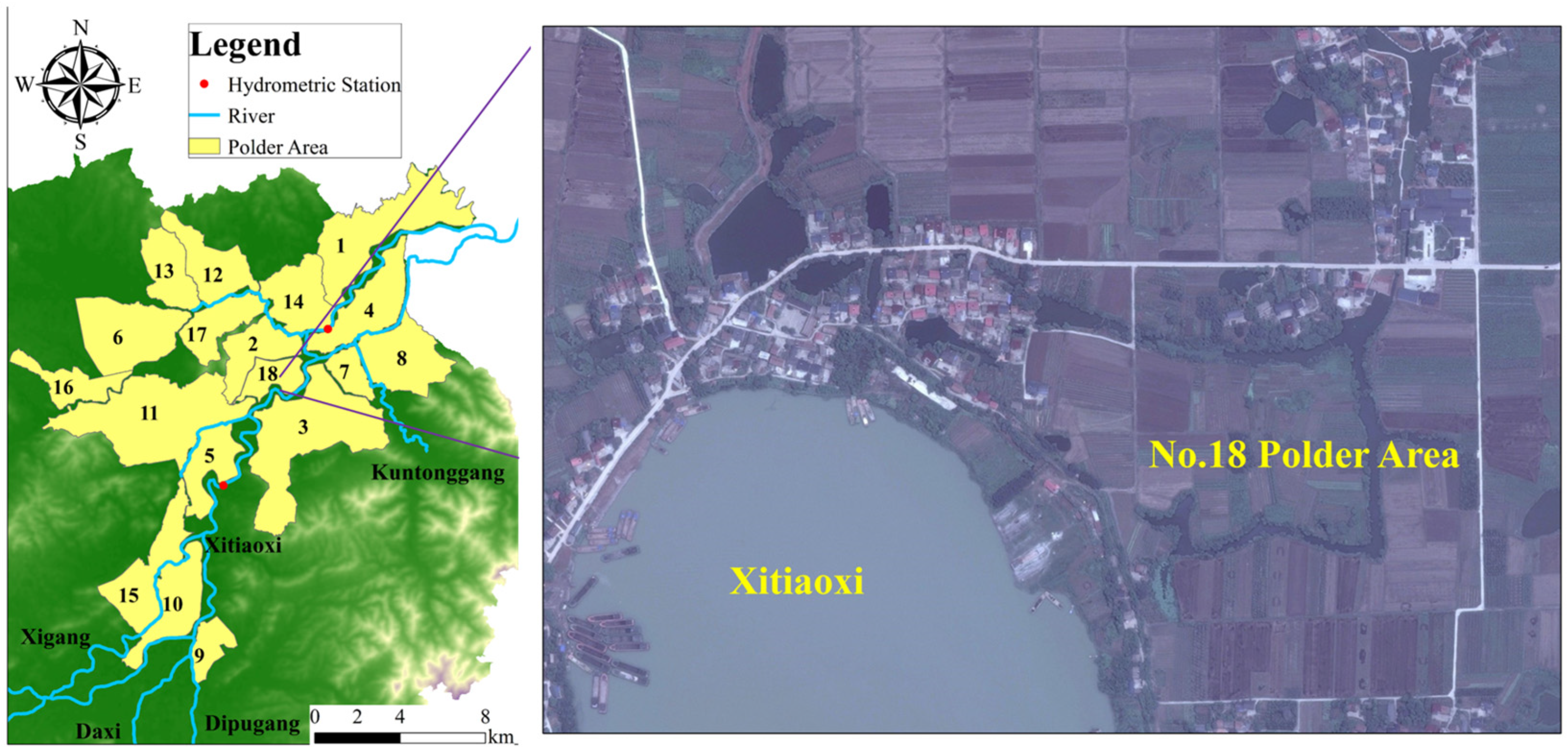
2.2. Polder Areas
2.3. Data
3. Methodology
3.1. Hydrodynamic Theories
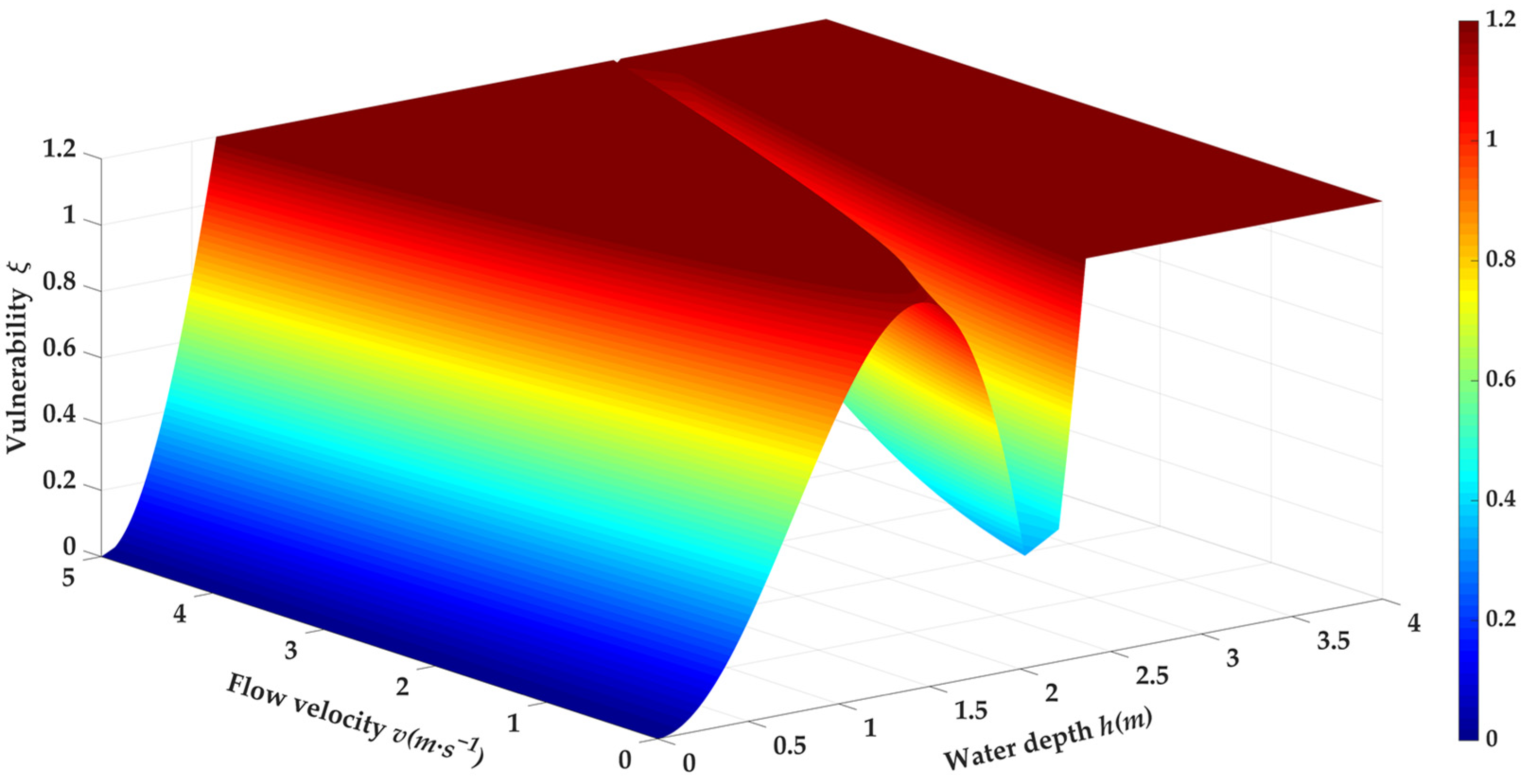
3.2. Depth–Velocity–Vulnerability Curve
4. Set of Hydrodynamic Model
4.1. Set of MIKE 11
4.2. Set of MIKE 21
4.3. Set of MIKE FLOOD
4.4. Verification of the Coupled Model
5. Results
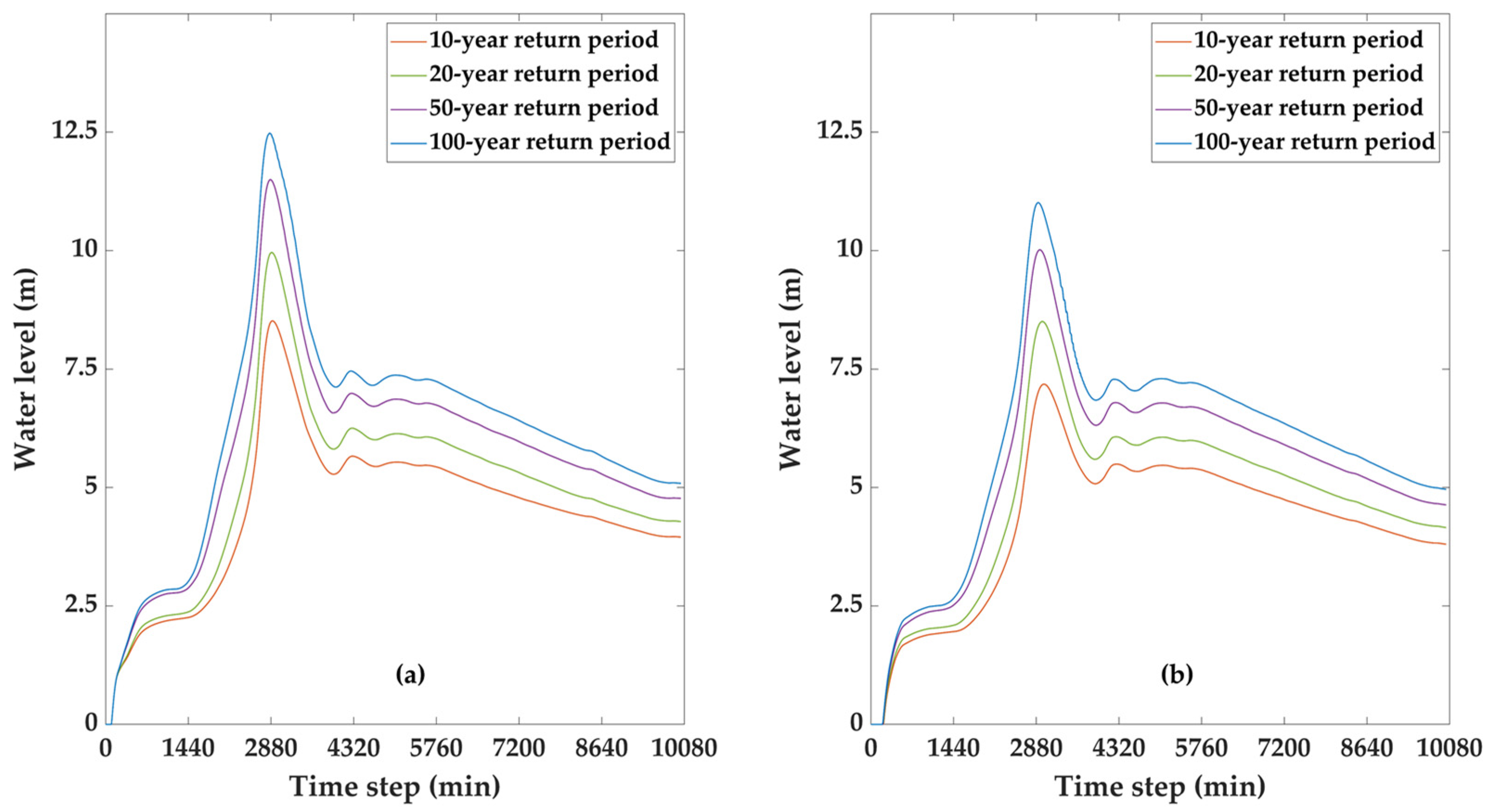
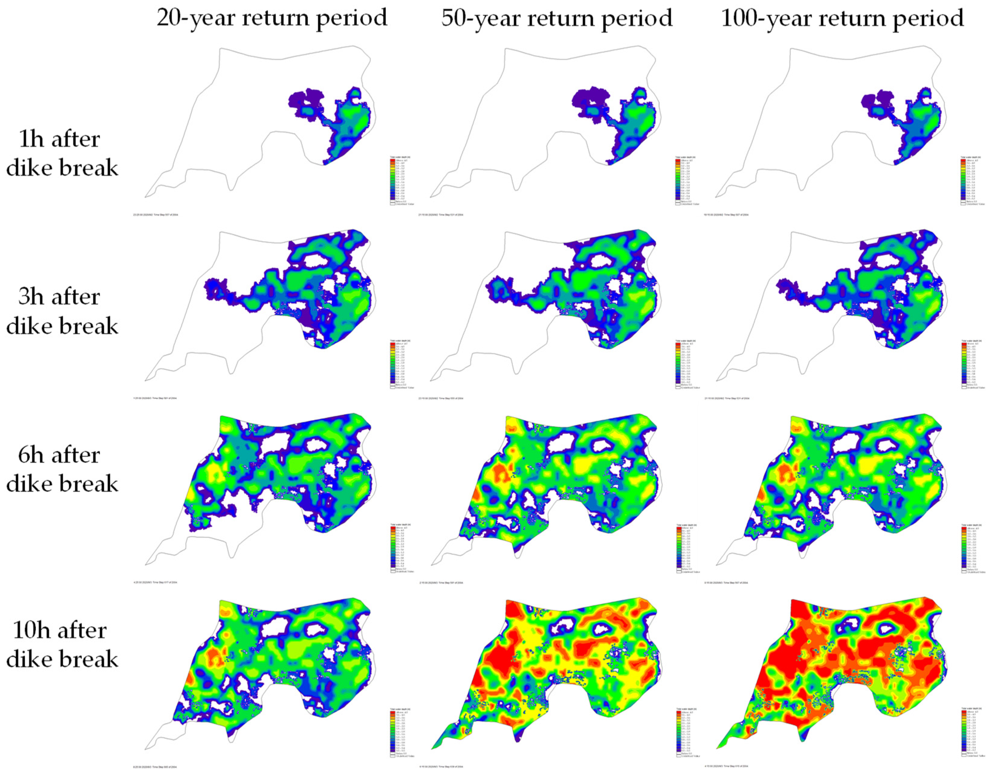
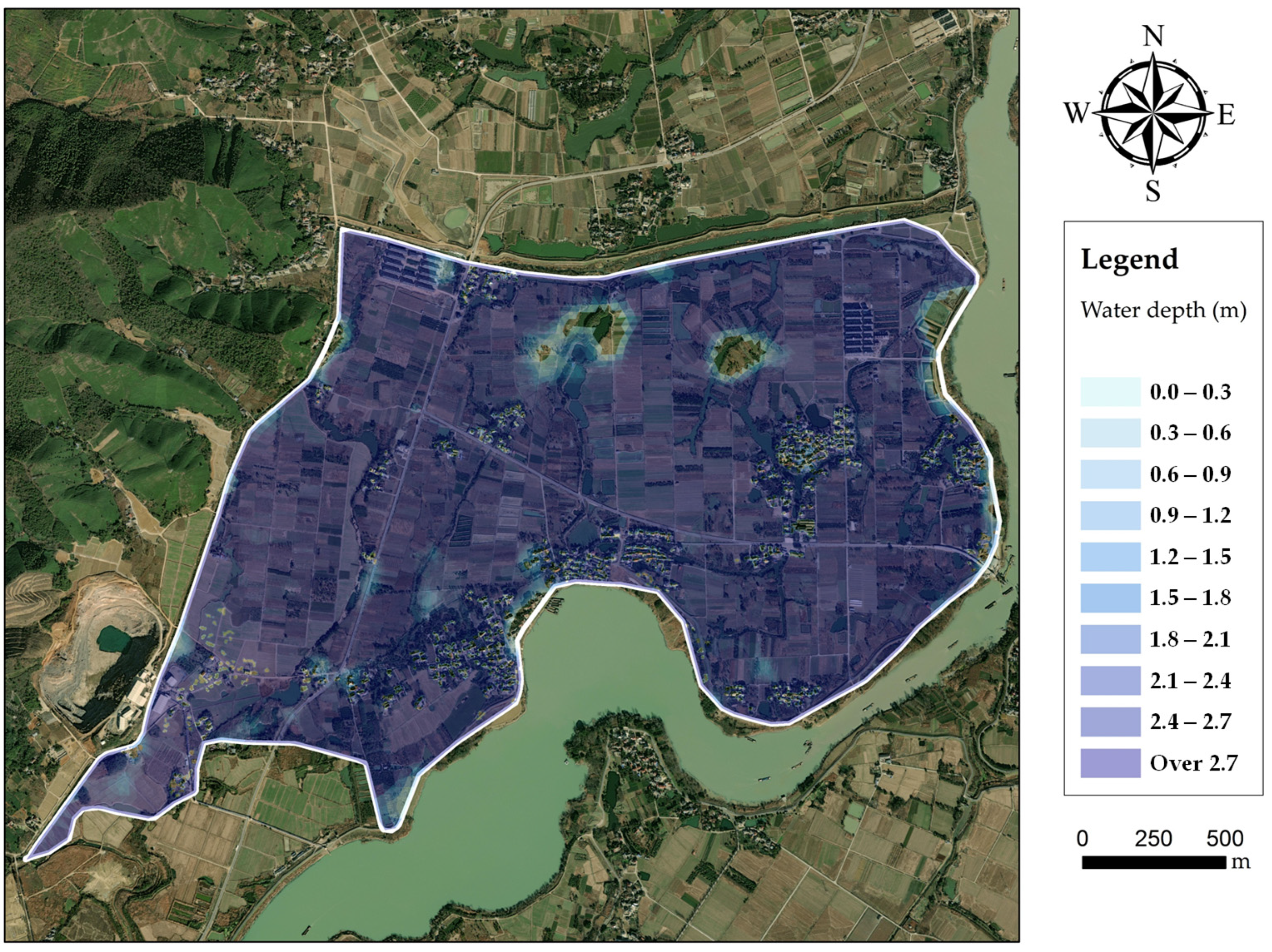
5.1. Flooding Analysis
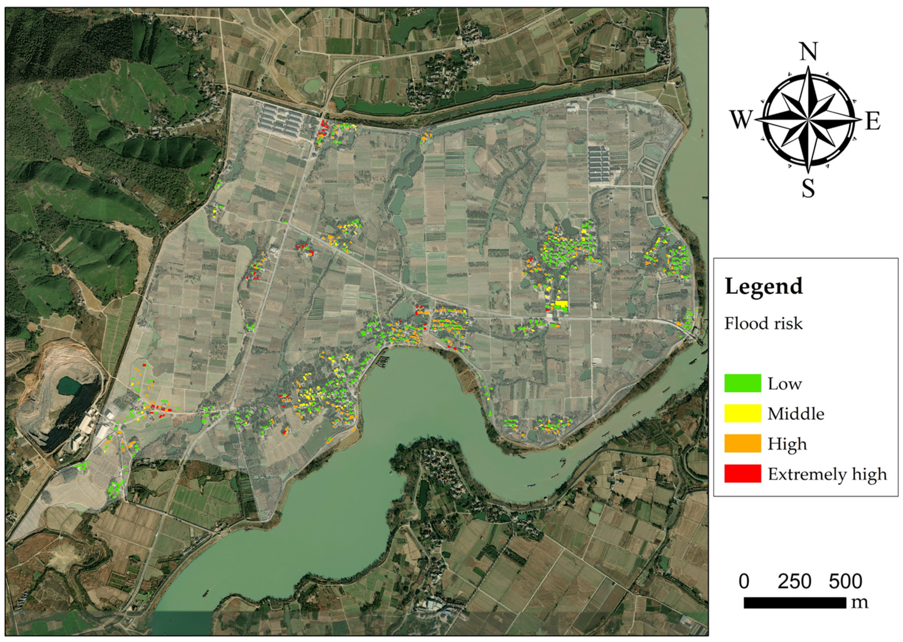
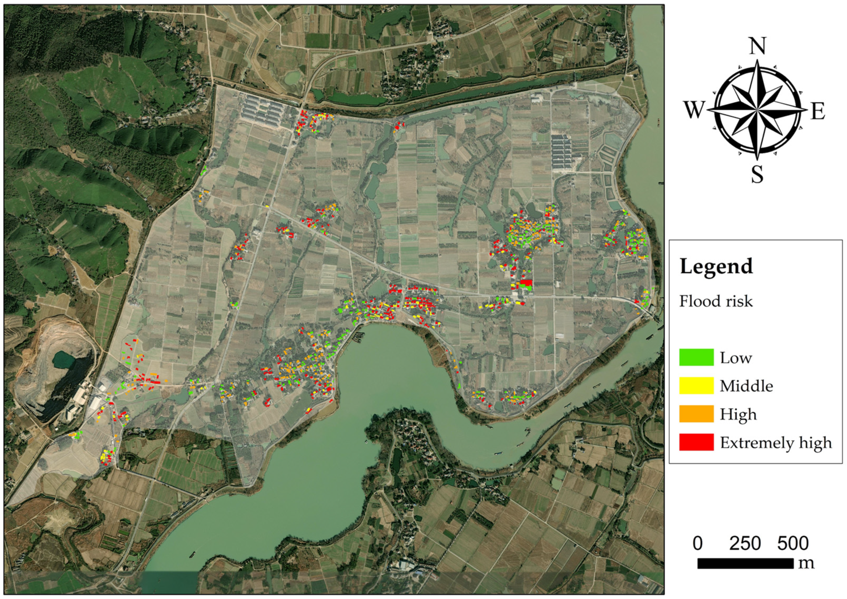
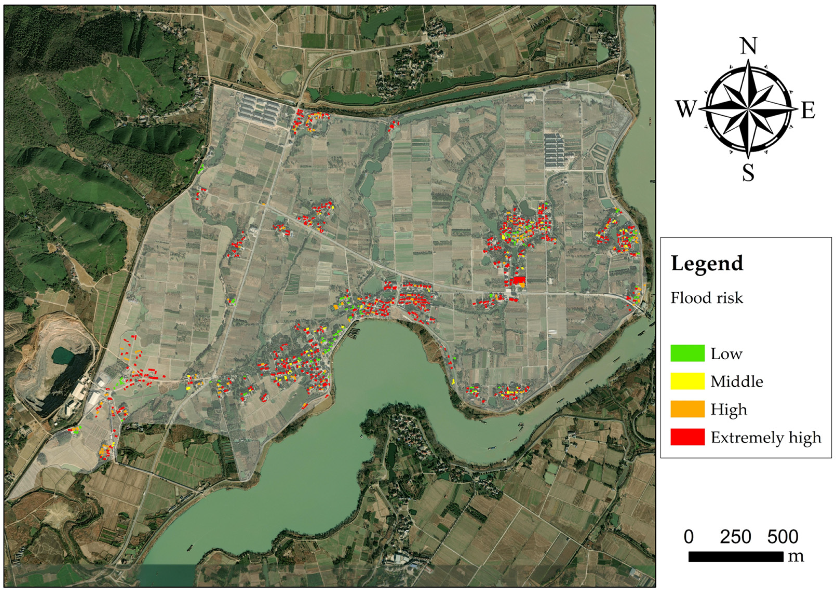
5.2. Flood Risk Assessment of Buildings
- Notice the structural safety of dikes. Floodwater can easily diffuse in the polder areas through the dike breaks, due to the lower terrain than the periphery. The assemblage of water neighboring the buildings leads to strong hydrostatic actions while the diffusion of that brings considerable hydrodynamic actions. However, unless the dikes were broken so limited floodwater would invade the polder, several pumps could be adequate.
- Take defensive measures around buildings. Bounding walls can reduce the impact between floodwater and buildings and are conducive to draining away floodwater.
- Avoid complete isolation caused by floodwater. Actually, strong hydrostatic actions occur only when there is a great water level difference between the exterior and interior. Consequently, appropriately allowing the floodwater to accumulate inside the building is significant in severe flood scenarios.
6. Discussion and Conclusions
6.1. Discussion
- The randomness of building parameters. The resistant capacity of buildings relies on a series of random variables, for instance, tensile strength and orientation. The desired method is to ascertain the probability distribution function (PDF) of each factor based on field surveys, physical modeling experiments, and numerical simulations. The vulnerability can be theoretically described as the conditional expectation of destruction probability.
- The destruction process is caused by a flood. Flood risk assessment concentrates not only on the ultimate limit state of buildings but also the damage ratio under different situations. Different failure stages correspond to different flood risks. Meanwhile targeted measures are in accordance with the failure stage of buildings. So, the destruction process is the bridge the risk assessment and damage reduction.
- The complex actions caused by a flood. Erosion actions, buoyancy actions, and scouring actions play important roles in the long-term flood impact. As for a certain flood, it is the hydrostatic actions and the hydrodynamic actions that bring about the damage to buildings directly. However, other flood actions can gradually weaken the resistant capacity of buildings over a long time scale. That is to say, inundation duration should be a concern more in the assessment of flooding areas.
6.2. Conclusions
Author Contributions
Funding
Institutional Review Board Statement
Data Availability Statement
Acknowledgments
Conflicts of Interest
References
- Hariri-Ardebili, M.A.; Lall, U. Superposed natural hazards and pandemics: Breaking dams, floods, and COVID-19. Sustainability 2021, 13, 8713. [Google Scholar] [CrossRef]
- Chinh, D.T.; Gain, A.K.; Dung, N.V.; Haase, D.; Kreibich, H. Multi-variate analyses of flood loss in Can Tho City, Mekong Delta. Water 2016, 8, 6. [Google Scholar] [CrossRef]
- Liu, Z.; Cai, Y.; Wang, S.; Lan, F.; Wu, X. Small and medium-scale river flood controls in highly urbanized areas: A whole region perspective. Water 2020, 12, 182. [Google Scholar] [CrossRef]
- Stefanidis, S.; Alexandridis, V.; Theodoridou, T. Flood Exposure of Residential Areas and Infrastructure in Greece. Hydrology 2022, 9, 145. [Google Scholar] [CrossRef]
- Chakraborty, J.; Collins, T.W.; Montgomery, M.C.; Grineski, S.E. Social and spatial inequities in exposure to flood risk in Miami, Florida. Nat. Hazards Rev. 2014, 15, 04014006. [Google Scholar] [CrossRef]
- Rakwatin, P.; Sansena, T.; Marjang, N.; Rungsipanich, A. Using multi-temporal remote-sensing data to estimate 2011 flood area and volume over Chao Phraya River basin, Thailand. Remote Sens. Lett. 2013, 4, 243–250. [Google Scholar] [CrossRef]
- Dao, D.A.; Kim, D.; Park, J.; Kim, T. Precipitation threshold for urban flood warning—An analysis using the satellite-based flooded area and radar-gauge composite rainfall data. J. Hydro-Environ. Res. 2020, 32, 48–61. [Google Scholar] [CrossRef]
- Ministry of Water Resources of the People’s Republic of China. Zhongguo Shuihan Zaihai Gongbao 2018; China Water & Power Press: Beijing, China, 2019. [Google Scholar]
- UN-Habitat. World Cities Report 2022: Envisaging the Future of Cities; United Nations Human Settlements Programme: Nairobi, Kenya, 2022. [Google Scholar]
- Chacowry, A.; McEwen, L.J.; Lynch, K. Recovery and resilience of communities in flood risk zones in a small island developing state: A case study from a suburban settlement of Port Louis, Mauritius. Int. J. Disaster Risk Reduct. 2018, 28, 826–838. [Google Scholar] [CrossRef]
- Milanesi, L.; Pilotti, M. Coupling flood propagation modeling and building collapse in flash flood studies. J. Hydraul. Eng.-ASCE 2021, 147, 04021047. [Google Scholar] [CrossRef]
- Zhu, S.; Dai, Q.; Zhao, B.; Shao, J. Assessment of population exposure to urban flood at the building scale. Water 2020, 12, 3253. [Google Scholar] [CrossRef]
- Mrozik, K.D. Problems of Local Flooding in Functional Urban Areas in Poland. Water 2022, 14, 2453. [Google Scholar] [CrossRef]
- Porter, J.R.; Shu, E.; Amodeo, M.; Hsieh, H.; Chu, Z.; Freeman, N. Community Flood Impacts and Infrastructure: Examining National Flood Impacts Using a High Precision Assessment Tool in the United States. Water 2021, 13, 3125. [Google Scholar] [CrossRef]
- Hudson, P.; Botzen, W.J.W.; Poussin, J.; Aerts, J.C.J.H. Impacts of flooding and flood preparedness on subjective well-being: A monetisation of the tangible and intangible impacts. J. Happiness Stud. 2019, 20, 665–682. [Google Scholar] [CrossRef]
- Ujeyl, G.; Rose, J. Estimating direct and indirect damages from storm surges: The case of Hamburg-Wilhelmsburg. Coast Eng. J. 2015, 57, 1540006. [Google Scholar] [CrossRef]
- Tobin, G.A. Floods: Physical processes and human impacts. Prof. Geogr. 1998, 51, 477–479. [Google Scholar]
- Zhu, J.; Dai, Q.; Deng, Y.; Zhang, A.; Zhang, Y.; Zhang, S. Indirect damage of urban flooding: Investigation of flood-induced traffic congestion using dynamic modeling. Water 2018, 10, 622. [Google Scholar] [CrossRef]
- Smith, D.I. Flood damage estimation—A review of urban stage-damage curves and loss functions. Water SA 1994, 20, 231–238. [Google Scholar]
- Penning-Rowsell, E.C.; Green, C.H.; Thompson, P.M.; Coker, S.M.; Tunstall, S.M.; Richards, C.; Parker, D.J. The Economics of Coastal Management: A Manual of Benefit Assessment Techniques (Nicknamed the Yellow Manual); Belhaven Press: London, UK, 1992. [Google Scholar]
- Kelman, I.; Spence, R. An overview of flood actions on buildings. Eng. Geol. 2004, 73, 297–309. [Google Scholar] [CrossRef]
- Papathoma-Kohle, M.; Keiler, M.; Totschnig, R.; Glade, T. Improvement of vulnerability curves using data from extreme events: Debris flow event in South Tyrol. Nat. Hazards 2012, 64, 2083–2105. [Google Scholar] [CrossRef]
- Thapa, S.; Shrestha, A.; Lamichhane, S.; Adhikari, R.; Gautam, D. Catchment-scale flood hazard mapping and flood vulnerability analysis of residential buildings: The case of Khando River in eastern Nepal. J. Hydrol.-Reg. Stud. 2020, 30, 100704. [Google Scholar] [CrossRef]
- Buchele, B.; Kreibich, H.; Kron, A.; Thieken, A.; Ihringer, J.; Oberle, P.; Merz, B.; Nestmann, F. Flood-risk mapping: Contributions towards an enhanced assessment of extreme events and associated risks. Nat. Hazards Earth Syst. Sci. 2006, 6, 485–503. [Google Scholar] [CrossRef]
- Penning-Rowsell, E.C.; Viavattene, C.; Pardoe, J.; Chatterton, J.; Parker, D.J.; Morris, J. The Benefits of Flood and Coastal Risk Management: A Handbook of Techniques-2010; Flood Hazard Research Centre, Middlesex University: London, UK, 2010. [Google Scholar]
- Scawthorn, C.; Flores, P.; Blais, N.; Seligson, H.; Tate, E.; Chang, S.; Mifflin, E.; Thomas, W.; Murphy, J.; Jones, C.; et al. HAZUS-MH flood loss estimation methodology: Damage and loss assessment. Nat. Hazards Rev. 2006, 7, 72–81. [Google Scholar] [CrossRef]
- Downton, M.W.; Miller, J.Z.B.; Pielke, R.A., Jr. Reanalysis of U.S. National Weather Service flood loss database. Nat. Hazards Rev. 2005, 6, 13–22. [Google Scholar] [CrossRef]
- Huizinga, J.; Moel, H.de.; Szewczyk, W. Global Flood Depth-Damage Functions: Methodology and the Database with Guidelines; European Commission, Joint Research Centre: Sevilla, Spain, 2017. [Google Scholar]
- Haider, S.; Saeed, U.; Shahid, M. 2D numerical modeling of two dam-break flood model studies in an urban locality. Arab. J. Geosci. 2020, 13, 682. [Google Scholar] [CrossRef]
- Clausen, L.K. Potential Dam Failure: Estimation of Consequences, and Implications for Planning. Master’s Thesis, Middlesex University, London, UK, 1989. [Google Scholar]
- Pistrika, A.K.; Jonkman, S.N. Damage to residential buildings due to flooding of New Orleans after hurricane Katrina. Nat. Hazards 2010, 54, 413–434. [Google Scholar] [CrossRef]
- Nadal, N.C.; Zapata, R.E.; Pagan, I.; Lopez, R.; Agudelo, J. Building damage due to riverine and coastal floods. J. Water Resour. Plan. Manag.-ASCE 2010, 136, 327–336. [Google Scholar] [CrossRef]
- De Risi, R.; Jalayer, F.; De Paola, F.; Iervolino, I.; Giugni, M.; Topa, M.E.; Mbuya, E.; Kyessi, A.; Manfredi, G.; Gasparini, P. Flood risk assessment for informal settlements. Nat. Hazards 2013, 69, 1003–1032. [Google Scholar] [CrossRef]
- Custer, R.; Nishijima, K. Flood vulnerability assessment of residential buildings by explicit damage process modelling. Nat. Hazards 2015, 78, 461–496. [Google Scholar] [CrossRef]
- Martins, L.; Silva, V. Development of a fragility and vulnerability model for global seismic risk analyses. Bull. Earthq. Eng. 2020, 19, 6719–6745. [Google Scholar] [CrossRef]
- Andrewwinner, R.; Chandrasekaran, S.S. Finite element and vulnerability analyses of a building failure due to landslide in Kaithakunda, Kerala, India. Adv. Civ. Eng. 2022, 2022, 5297864. [Google Scholar] [CrossRef]
- Ferrito, T.; Milosevic, J.; Bento, R. Seismic vulnerability assessment of a mixed masonry-RC building aggregate by linear and nonlinear analyses. Bull. Earthq. Eng. 2016, 8, 2299–2327. [Google Scholar] [CrossRef]
- Mazzorana1, B.; Simoni, S.; Scherer, C.; Gems, B.; Fuchs, S.; Keiler, M. A physical approach on flood risk vulnerability of buildings. Hydrol. Earth Syst. Sci. 2014, 18, 3817–3836. [Google Scholar] [CrossRef]
- Papathoma-Kohle, M.; Schlogl, M.; Dosser, L.; Roesch, F.; Borga, M.; Erlicher, M.; Keiler, M.; Fuchs, S. Physical vulnerability to dynamic flooding: Vulnerability curves and vulnerability indices. J. Hydrol. 2022, 607, 127501. [Google Scholar] [CrossRef]
- Lagomarsino, S.; Cattari, S.; Ottonelli, D.; Giovinazzi, S. Earthquake damage assessment of masonry churches: Proposal for rapid and detailed forms and derivation of empirical vulnerability curves. Bull. Earthq. Eng. 2019, 17, 3327–3364. [Google Scholar] [CrossRef]
- Wang, Y.; Liu, G.; Guo, E.; Yun, X. Quantitative agricultural flood risk assessment using vulnerability surface and copula functions. Water 2018, 10, 1229. [Google Scholar] [CrossRef]
- Vandenbohede, A.; Hinsby, K.; Courtens, C.; Lebbe, L. Flow and transport model of a polder area in the Belgian coastal plain: Example of data integration. Hydrogeol. J. 2011, 19, 1599–1615. [Google Scholar] [CrossRef]
- Niroshinie, M.A.C.; Nihei, Y.; Ohtsuki, K.; Okada, S. Flood inundation analysis and mitigation with a coupled 1D-2D hydraulic model: A case study in Kochi, Japan. J. Disaster Res. 2015, 10, 1099–1109. [Google Scholar] [CrossRef]
- Tansar, H.; Akbar, H.; Aslam, R.A. Flood inundation mapping and hazard assessment for mitigation analysis of local adaptation measures in Upper Ping River Basin, Thailand. Arab. J. Geosci. 2021, 14, 2531. [Google Scholar] [CrossRef]
- Li, J.; Zhang, B.; Li, Y.; Li, H. Simulation of rain garden effects in urbanized area based on mike flood. Water 2018, 10, 860. [Google Scholar] [CrossRef]
- Postacchini, M.; Zitti, G.; Giordano, E.; Clementi, F.; Darvini, G.; Lenci, S. Flood impact on masonry buildings: The effect of flow characteristics and incidence angle. J. Fluids Struct. 2019, 88, 48–70. [Google Scholar] [CrossRef]
- Fang, Q.; Liu, S.; Zhong, G.; Liang, J.; Zhen, Y. Experimental investigation of extreme flood loading on buildings considering the shadowing effect of the front building. J. Hydraul. Eng.-ASCE 2022, 148, 04022007. [Google Scholar] [CrossRef]
- Sun, Y. Numerical Simulation Study on Mountain Rural Buildings Due to Flood Impact. Master’s Thesis, Dalian University of Technology, Dalian, China, 2011. [Google Scholar]
- USACE (United States Army Corps of Engineers). Flood Proofing: Techniques, Programs, and Reference; National Flood Profing Committee: Washington, DC, USA, 2017.
- Xiao, S.; Li, H. Impact of flood on a simple masonry building. J. Perform. Constr. Facil. 2013, 27, 550–563. [Google Scholar] [CrossRef]
- Ettinger, S.; Mounaud, L.; Magill, C.; Yao-Lafourcade, A.F.; Thouret, J.C.; Manville, V.; Negulescu, C.; Zuccaro, G.; De Gregorio, D.; Nardone, S.; et al. Building vulnerability to hydro-geomorphic hazards: Estimating damage probability from qualitative vulnerability assessment using logistic regression. J. Hydrol. 2015, 541, 563–581. [Google Scholar] [CrossRef]
- Moreira, L.L.; de Brito, M.M.; Kobiyama, M. Effects of different normalization, aggregation, and classification methods on the construction of flood vulnerability indexes. Water 2021, 13, 98. [Google Scholar] [CrossRef]
- Zhen, Y.; Liu, S.; Zhong, G.; Zhou, Z.; Liang, J.; Zheng, W.; Fang, Q. Risk assessment of flash flood to buildings using an indicator-based methodology: A case study of mountainous rural settlements in southwest China. Front. Environ. Sci. 2022, 10, 931029. [Google Scholar] [CrossRef]


| Typhoon | Item | Observed Value | Simulated Value | Error |
|---|---|---|---|---|
| Morakot | Water level at HHS | 7.61 m | 7.63 m | +0.02 m |
| Water level at MHS | 6.70 m | 6.69 m | −0.01 m | |
| Fitow | Water level at HHS | 8.59 m | 8.58 m | −0.01 m |
| Water level at MHS | 7.39 m | 7.42 m | +0.03 m | |
| Discharge at HHS | 1930 m3/s | 1991 m3/s | +61 m3/s |
Publisher’s Note: MDPI stays neutral with regard to jurisdictional claims in published maps and institutional affiliations. |
© 2022 by the authors. Licensee MDPI, Basel, Switzerland. This article is an open access article distributed under the terms and conditions of the Creative Commons Attribution (CC BY) license (https://creativecommons.org/licenses/by/4.0/).
Share and Cite
Liu, S.; Zheng, W.; Zhou, Z.; Zhong, G.; Zhen, Y.; Shi, Z. Flood Risk Assessment of Buildings Based on Vulnerability Curve: A Case Study in Anji County. Water 2022, 14, 3572. https://doi.org/10.3390/w14213572
Liu S, Zheng W, Zhou Z, Zhong G, Zhen Y, Shi Z. Flood Risk Assessment of Buildings Based on Vulnerability Curve: A Case Study in Anji County. Water. 2022; 14(21):3572. https://doi.org/10.3390/w14213572
Chicago/Turabian StyleLiu, Shuguang, Weiqiang Zheng, Zhengzheng Zhou, Guihui Zhong, Yiwei Zhen, and Zheng Shi. 2022. "Flood Risk Assessment of Buildings Based on Vulnerability Curve: A Case Study in Anji County" Water 14, no. 21: 3572. https://doi.org/10.3390/w14213572
APA StyleLiu, S., Zheng, W., Zhou, Z., Zhong, G., Zhen, Y., & Shi, Z. (2022). Flood Risk Assessment of Buildings Based on Vulnerability Curve: A Case Study in Anji County. Water, 14(21), 3572. https://doi.org/10.3390/w14213572