Article

Simpler Is Better—Calibration of Pipe Roughness in Water Distribution Systems

1
Department of Infrastructure Engineering, The University of Melbourne, Melbourne, VIC 3010, Australia
2
School of Civil, Environmental & Mining Engineering, The University of Adelaide, Adelaide, SA 5005, Australia
3
Lower Murray Water, Mildura, VIC 3500, Australia
*
Author to whom correspondence should be addressed.
Water 2022, 14(20), 3276; https://doi.org/10.3390/w14203276
Submission received: 9 September 2022 / Revised: 1 October 2022 / Accepted: 14 October 2022 / Published: 17 October 2022
(This article belongs to the Special Issue Optimization Studies for Water Distribution Systems)

Abstract

:
Hydraulic models of water distribution systems (WDSs) need to be calibrated, so they can be used to help to make informed decisions. Usually, hydraulic model calibration follows an iterative process of comparing the simulation results from the model with field observations and making adjustments to model parameters to make sure an acceptable level of agreement between predicted and measured values (e.g., water pressure) has been achieved. However, the manual process can be time-consuming, and the termination criterion relies on the modeler’s judgment. Therefore, various optimization-based calibration methods have been developed. In this study, three different optimization methods, i.e., Sequential Least Squares Programming (SLSQP), a Genetic Algorithm (GA) and Differential Evolution (DE), are compared for calibrating the pipe roughness of WDS models. Their performance is investigated over four different decision variable set formulations with different levels of discretization of the search space. Results obtained from a real-world case study demonstrate that compared to traditional engineering practice, optimization is effective for hydraulic model calibration. However, a finer search space discretization does not necessarily guarantee better results; and when multiple methods lead to similar performance, a simpler method is better. This study provides guidance on method and formulation selection for calibrating WDS models.

1. Introduction

Hydraulic models have been widely used for the planning, design, operation, maintenance and management of water distribution systems (WDSs) by water utilities to assist in the evaluation of system performance and the assessment of design or operating options [1,2,3,4,5]. A WDS hydraulic model should always be first calibrated prior to being used in any decision-making process [6,7,8,9,10], as the mismatch between the model-predicted and field-observed behaviors normally exists because of model uncertainty [8,11,12] and sometimes the absence of system details.
Hydraulic model calibration involves an iterative process of comparing the simulation results from the model with the field observations and making adjustments to model input to improve the match between predicted and measured values until an acceptable level of agreement has been achieved [2,3,4,5,9,13,14,15,16]. A number of model parameters have been considered in the calibration process, such as pipe roughness, nodal demands, characteristics and the operational status of pipes, pumps and valves [2,3,5,16]. Among these calibration parameters, pipe roughness values are commonly estimated for static calibration [16], considering their high impact on the system uncertainty and the associated difficulties in the direct measurement of the actual values [17].
Common approaches for WDS hydraulic model calibration can be grouped into two major categories: manual (trial-and-error) and automatic calibration approaches [2,4,15,18]. In the traditional manual calibration approach based on trial-and-error [3,4,19,20], unknown calibration parameters are adjusted manually by modelers or engineers at each iteration of the trials until a certain degree of model accuracy has been achieved. Manual calibration is normally considered when the initial gaps between the observed data and the modeled results are significant [2]. Major anomalies or accuracy of initial parameters and input data might be identified in this process [4,18]. The trial-and-error approach can be very time-consuming and tedious as the judgment and adjustment have to be repeated manually many times [3,21]. The speed of convergence of the iterative method is very slow, with no guarantee of desirable results obtained [4,21].
Considering the limitations of the manual approach, automatic calibration methods have been developed to deal with the larger number of unknowns in a realistic WDS and to achieve a higher level of efficiency and accuracy [2,3,5]. There are two common categories of methods for automatic calibration: numerical and optimization-based (or implicit [4]) methods. Numerical methods mainly involve the estimation of calibration parameters by solving a set of mass balance and energy equations directly [2]. For example, early explicit calibration methods involve solving an extended series of steady-state hydraulic equations [4,5,6,22,23,24]. However, it requires that the number of calibration parameters must match the number of observations (field measurements). Additionally, errors in measurements are often neglected [16]. The optimization-based methods mainly involve the estimation of calibration parameters by minimizing the differences between the observations and model-simulated results through the use of an optimization algorithm coupled with the hydraulic simulation model [4,8]. This method has been widely investigated [3,16,25,26,27,28,29,30,31,32].
There are two common categories of optimization-based techniques that have been used for hydraulic model calibration: deterministic (or classic) and metaheuristic algorithms [33,34,35]. Deterministic algorithms such as gradient-based algorithms mainly consist of linear, nonlinear and dynamic programming [35,36]. For instance, gradient-based algorithms are dominant in non-evolutionary optimization methods. A number of existing studies used gradient-based methods in the model calibration problems, such as the general reduced gradient (GRG) method [21,37], the Gauss-Newton method [38,39], and the Levenberg–Marquardt method [40]. The deterministic methods are computationally efficient [41] and able to locate an optimal solution. However, they sometimes converge to locally optimal solutions [35].
Metaheuristic algorithms, such as Evolutionary Algorithms (EAs) have been widely applied in the calibration of WDS models since their initial use in WDS model calibration by Savic and Walters [30]. EAs have been found to perform well in solving complex problems with many decision variables and constraints [42]. They have the ability to find the (near-) optimal solutions due to the exploratory nature of metaheuristics [43]. Their application to both continuous and discrete search space, as well as the ability to deal with multiple objective functions simultaneously, are also their strengths. However, the main limitation is related to the high computational cost, especially for larger optimization problems such as the calibration of complex WDS models [2,27] as the optimization process involves frequent solving of nonlinear hydraulic equations [44]. Therefore, it is challenging to locate (near-) optimal solutions considering the large search space these problems have [45]. Consequently, some studies have considered grouping decision variables based on their similar properties or characteristics, thus reducing the size of the optimization problem (the number of decision variables) and improving the efficiency in finding (near-) optimal solutions [2,27,32]. Another downside of metaheuristic algorithms in calibration is often based on limited pressure measurement data that is usually available to calibrate a hydraulic model, which can lead to a problem that has multiple possible solutions [16,46,47]. This issue is addressed in this study by considering 10 simulations with 10 different random seeds, which encourages the exploration of the search space.
In this paper, three different optimization methods, i.e., Sequential Least Squares Programming (SLSQP), a Genetic Algorithm (GA) and Differential Evolution (DE), are compared for calibrating the pipe roughness of WDS hydraulic models. Their performance is investigated over four different decision variable set formulations where different numbers of decision variables are used to represent different levels of discretization of the search space. The main contribution of this study is to provide guidance on the selection of the combination of optimization methods and decision variable set formulations in terms of defining decision variables when calibrating WDS hydraulic models. A real-world pressurized irrigation system in Victoria, Australia has been selected as the case study system.

2. Methods

2.1. Calibration Process

The hydraulic model calibration process used in this paper is demonstrated in Figure 1. First, the original network model needs to be simplified to make sure only pipes that can have an impact on the calibration process (e.g., pipes upstream of pressure sensors) are selected to form the pruned network model. Other branches and pipes are removed to reduce redundancy in the model. Second, the model calibration problem is then formulated as an optimization problem to minimize the differences between field-observed and model-predicted pressures at various monitoring sites by adjusting pipe roughness values. Third, the optimization is conducted, and a final calibrated model can be then obtained.

2.2. Model Simplification

The process of model simplification mainly involves selecting pipes and corresponding roughness values that will have an impact on the readings of pressure sensors that are used for model calibration. A pruned network will result in a reduced number of pipes. The model simplification follows three steps. First, pressure sensor locations are identified. Second, each pressure sensor in treed portions of the network is considered in turn. If the pressure sensor in a treed portion of the network has no other pressure sensors downstream, then all of the downstream pipes from that pressure sensor are removed from the calibration. Changes in roughness values of these removed branched pipes would have had no impact on the pressure sensor readings. Third, pressure sensors in looped portions of the network are considered in turn. Pipes in each loop are retained in the calibration process if they are upstream of at least one pressure sensor. In summary, all pipes downstream of a pressure sensor that will have no influence on the calibration are removed to form the pruned network. When the pruned network model has been calibrated, calibrated pipe roughness values will be assigned to those pipes that were deleted in the model simplification process according to materials and diameters. The model simplification concept has been considered in a number of studies such as Zanfei, Menapace, Santopietro and Righetti [47]. Its application can save significant computational resources by reducing the number of decision variables at the initial stage of model calibration.

2.3. Optimization Problem Formulation

The model calibration problem (i.e., calibration of pipe roughness) has been formulated as an optimization problem. Considering a good measure of accuracy, the root mean squared error (RMSE) has previously been widely considered in hydraulic model calibration problems [4,48,49,50]. Although it may reduce the impact of extreme errors, the use of RMSE is considered sufficient for the aim of this study which is to investigate the impact of the combination of different optimization algorithms and decision variable set formulations on hydraulic model calibration. Therefore, the overall optimization objective is to minimize the average of root mean square error (RMSE) values between the measured and the predicted pressures at the different pressure monitoring sites, which is given by
m i n   [ 1 N i = 1 N ( R M S E i ) ]
where N = the number of pressure sensors within the network. The individual R M S E i at each pressure measurement site is given by
R M S E i = t = 1 T ( p o , t p m , t ) 2 T
where T = number of time steps, indexed t ; p o , t = field-observed pressure; and p m , t = model-predicted pressure.

2.4. Decision Variable Formulations

In this paper, pipe roughness heights ( ε in mm for the Darcy-Weisbach friction factor) of different pipes (or groups of pipes) are regarded as the decision variables. In order to identify appropriate pipe roughness values to better replicate the hydraulic responses in real operations, four different ways (i.e., decision variable set formulations) for defining the number of decision variables have been investigated (Formulations 1 to 4 in Table 1). In this way, the impact of using different ways of grouping pipe roughness values on the optimization results can be further investigated. In Formulation 1, the roughness value of every single pipe in the pruned network is regarded as a decision variable, so the number of decision variables is equal to the number of pipes in the pruned network. In Formulation 2, it is assumed that pipes that are constructed of the same material will have the same roughness values. Therefore, the number of decision variables is equal to the number of pipe material types in the network. This formulation would not be appropriate if there was only one pipe material for the entire network under consideration. In Formulation 3, besides pipe materials, pipe diameters have also been incorporated in defining decision variables. For the same pipe material, it is assumed that pipes with the same diameters have the same roughness values, as the pipe diameter has an impact on the Darcy-Weisbach friction factor and potential biofilm growth (particularly in raw water delivery systems) which may affect pipe roughness heights [51,52,53]. In Formulation 4, pipes are grouped based on both their materials and velocities which are estimated based on the potential maximum flow of each pipe under peak demand loading cases and known pipe diameters. In other words, for pipes made from the same material, it is assumed that pipes with the same or similar velocities have the same pipe roughness values and are grouped as one decision variable. The pipe velocity has an impact on the Reynolds number when calculating the Darcy-Weisbach friction factor.

2.5. Optimization Methods

The selection of optimization methods depends on the complexity of the problem, the purpose of the model calibration, and the available packages or tools [4]. There is no formal agreement on which optimization technique is better for a specific calibration problem as trade-offs (e.g., performance and efficiency) often exist when comparing different options [4]. In this paper, three different optimization methods have been considered and compared. They are (1) a Sequential Least Squares Programming (SLSQP) algorithm, (2) a Genetic Algorithm (GA) and (3) a Differential Evolution (DE) algorithm.
The Sequential Least Squares Programming (SLSQP) algorithm was established based on the Han–Powell quasi-Newton method, and Lawson and Hanson’s non-negative least squares (NNLS) nonlinear solver [54]. As an expansion of the quadratic programming algorithm, SLSQP is commonly considered in the minimization problems subject to equality or inequality constraints, such as the minimization problem that is subject to the lower and upper bounds of pipe roughness values in this study. Considering its efficiency in solving constrained nonlinear optimization problems [54], SLSQP was selected as a typical gradient-based algorithm in this study.
Genetic Algorithms (GAs) and the Differential Evolution (DE) algorithm have been used as global optimization methods to find the optimal solutions to this calibration problem. As a robust optimization algorithm [3], have the ability to handle real-world complex networks, locate (near-) optimal solutions and easily incorporate additional decision variables and constraints [4,33]. Therefore, they have been widely used in the calibration of WDS models. In a GA optimization process, solutions are selected based on Darwin’s natural evolution principles [55]. In the model calibration process, an initial set of solutions (e.g., pipe roughness values) are generated by the GA. Then, a hydraulic model simulates the hydraulic grade line (HGL) (or nodal heads) and flows in each trial solution network within the population of solutions. A fitness value is computed then for the set of solutions based on the difference between the field measurements and the model-predicted results. In the GA, the solutions are ranked according to the fitness values. The Differential Evolution (DE) algorithm as one of the EAs was introduced by Storn and Price [56]. The DE algorithm is considered as a robust global optimization algorithm to tackle large-scale continuous optimization problems [56,57,58,59]. Additionally, DE algorithms converge well in comparison with some other evolutionary algorithms [58]. The generation of a new solution in the DE is the process of combining several solutions with the candidate solution [58].
For this study, the SLSQP is implemented using the Python-based optimizer SciPy.; and the GA and DE are customized and implemented in the Python-based optimization tool ‘pymoo’ [60]. A Python wrapper ‘owa-epanet 2.2.4’ developed by Open Water Analytics [61] was used together with the EPANET Programmer’s Toolkit [62] to link the optimizer to the EPANET hydraulic model. In addition, all optimization runs were conducted on the University of Melbourne’s Spartan High-Performance Computing (HPC) system, which combines a high-performance bare-metal computing with GPGPUs for various uses. The physical partition on Spartan HPC has 82 nodes equipped with 5904 cores (Intel(R) Xeon(R) Gold 6254 CPU @ 3.10 GHz) in total. The maximum RAM per node is about 1483 GB.

2.6. Common Engineering Practice and Model Validation

Results (the objective function values) obtained using optimization methods are compared to the engineering practice of selecting pipe roughnesses. Commonly used pipe roughness values (according to pipe materials) by water utilities based on engineering experience have also been input into the hydraulic model to simulate pressures at monitoring sites. Then, the objective function values (the average of RMSE values between observed and simulated pressures) were then calculated and compared with the results obtained using optimization methods.
Once a WDS hydraulic model has been calibrated, it is highly recommended to verify the accuracy through a model validation process by comparing modeled results with field-observed data from a different period of time [15,63]. Model validation is also an important step to verify the reliability of the calibration process and validate the model performance, which is not always considered in past calibration studies. In this paper, independent validation data has been selected to perform model validation.

3. Case Study System

3.1. System Overview

The Robinvale High-Pressure System (RVHPS) has been selected as the case study system, which is managed by the local water authority Lower Murray Water (LMW) in Victoria, Australia. The system is located on the south bank of the Murray River in north-western Victoria, Australia, covering an irrigation area of about 2700 hectares [64]. The major crop planted in this area is table grapes [65] which require a large amount of water for irrigation and cooling, particularly during the peak season. Water is pumped from the Murray River and delivered to customers by the Robinvale high-pressure pump station predominantly for irrigation and some also for domestic and stock (D&S) water use.
The Robinvale irrigation network was fully pipelined with the commissioning of the current system in October 2010. The layout of the system is shown in Figure 2. The current system delivers water to approximately 244 irrigation outlets and 210 small-diameter D&S outlets in the system. Irrigation water needs to be ordered in advance, while D&S water may be used from any of the outlets in the network without an order.
Water is pumped from the Murray River by the Robinvale high-pressure pump station located in the northeast of the network. There is no water treatment plant or storage tank within the system. The pumped water is delivered with a pressure head at the pump station ranging from 80 m to 105 m via two DN1200 MSCL (mild steel cement mortar lined) rising mains and a DN1400 GRP (glass reinforced plastic) main, and then distributed to smaller pipes. The system is comprised of approximately 77 km of pipes with nominal diameters ranging from DN80 to DN1400. Most of the pipes were installed in 2010 and made of four types of materials including MSCL, GRP, DICL (ductile iron cement mortar lined) and mPVC (modified polyvinyl chloride). In addition, the Robinvale high-pressure pump station is comprised of five identical main pumps for delivering larger flows, and four identical smaller jacking pumps to deliver lower flow rates and to re-pressurize the system for transition purposes. All pumps in parallel are controlled by variable speed drives (VSDs).

3.2. Existing Hydraulic Model

There was currently an uncalibrated EPANET hydraulic model available for the system. The EPANET model consists of 433 pipes with pipe length ranging from 0.7 m to 1359 m. Pipe roughnesses may have changed over the years since 2010 due to the nature of raw water delivery and the aging of pipes. Therefore, it was important to update and calibrate the model first to improve its accuracy before the model could be used to develop control strategies.
A number of updates to the existing EPANET model have been made before the calibration process. These model updates include changes made to nodes, pipes and pumps to reflect the configuration of the up-to-date network. The base demand and demand pattern of each irrigation outlet is calculated individually to reflect the actual water consumption during the calibration period. Moreover, a dummy PRV with simple control rules has been added downstream of the pumps to simulate the measured system pressures for the purpose of pipe roughness calibration.

3.3. Data Collection and Processing

3.3.1. Data Monitoring

In the Robinvale irrigation system, each irrigation outlet has a flow meter installed, with the real-time irrigation flow data monitored remotely using a SCADA system. Therefore, each outlet has a unique irrigation demand pattern during the calibration period. As shown in Figure 2 above, there are six permanent pressure sensors installed in the system, with one (Sys_Pres) located just out of the pump station and the other five (RTU1 to 5) across the network. In addition, a permanent flow meter (Sys_Flow) was installed on each of the two rising mains out of the pump station, measuring the total flow into the system. In addition, the pressure sensor accuracy is ±0.2% (approximately ±3.2 kPa).

3.3.2. Selection of Calibration and Validation Period

Data collection over an extended period is suggested in the WDS model calibration process to improve the model accuracy [29]. Additionally, the measured data is considered to be satisfactory when the error in the measurement of head loss is considerably smaller than the head loss itself [32,67]. Therefore, it is highly recommended to collect calibration and validation data during periods with peak demands [2,15,63,67,68,69] when the head loss is considered to be more sensitive to the variation in pipe roughness values. In addition, monitoring data availability and quality should also be taken into account for data selection. In this paper, 28 December 2019 has been selected as the calibration period, considering the high demand and the good quality of both flow and pressure data. The model validation period was selected as 19 December 2019 as one of the days that have the highest irrigation water demands, with the second-best quality pressure and flow data.

3.3.3. Data Pre-Processing

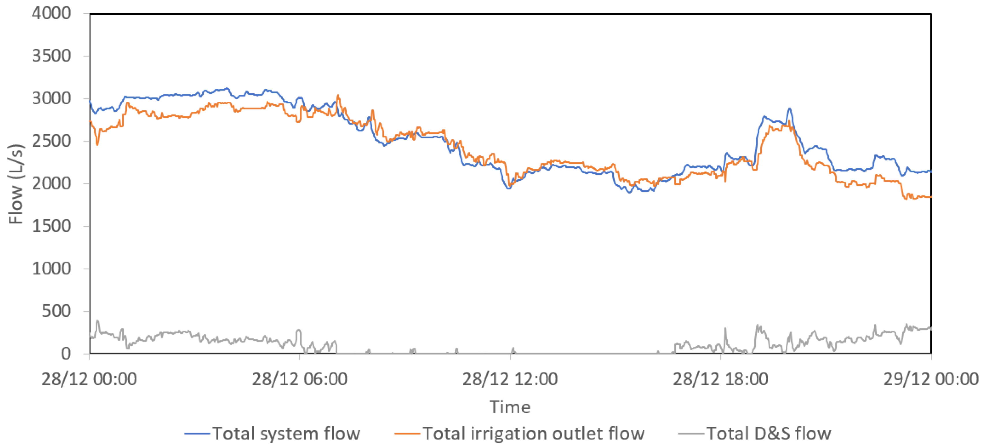
The data were pre-processed before the calibration process was carried out. First, all measured pressure and flow data have been interpolated into a regular 1 min time step which is smaller than the original interval of 144 s in the raw data. This makes the result comparison easier and ensures the accuracy of data interpolation. Second, as the D&S water consumption of each outlet is not measured in real-time, the total D&S demand is estimated by subtracting the sum of the real demand of each individual outlet from the total system flow observed at the pump station at each time step during the calibration period. The individual D&S demand pattern of each outlet is assumed to be the same as the total D&S demand pattern while the proportion of individual base demand is estimated according to the manual meter readings for each D&S outlet in the three months when the calibration period occurred. Figure 3 shows the time series of all categories of demands for the calibration period. Third, the observed system pressures just downstream of the pump station are replicated in the EPANET model as the initial condition to eliminate the impact of pump operations on the calibration results, as the pipe roughness in this paper is regarded as the main parameter to be calibrated. Further, through investigation, monitoring errors have been identified and corrected at the five pressure monitoring sites before calibration.
Through a number of preliminary EPANET model simulation runs, large vertical shifts between the field measurements and model-simulated pressures were identified at Pressure Sensor Number 2 (RTU2), 3 (RTU3) and 5 (RTU5). Particularly for RTU2, the observed Hydraulic Grade Line (HGL) was consistently about 10 m higher than the system HGL, which warrants further error investigation. Theoretically, under a zero-flow condition, the difference between the pressures of two nodes is expected to be equal to the difference between the elevations of the two. Therefore, after making the comparison under several historical static-pressure (near-zero flow) conditions, constant monitoring offset errors were identified to be 0.2 m, −12.6 m, 3.0 m, 0.9 m and 3.5 m for RTU1 to 5, respectively. Additionally, as the sensor elevations were surveyed and confirmed to be accurate, the corresponding errors were corrected at the five RTU locations.
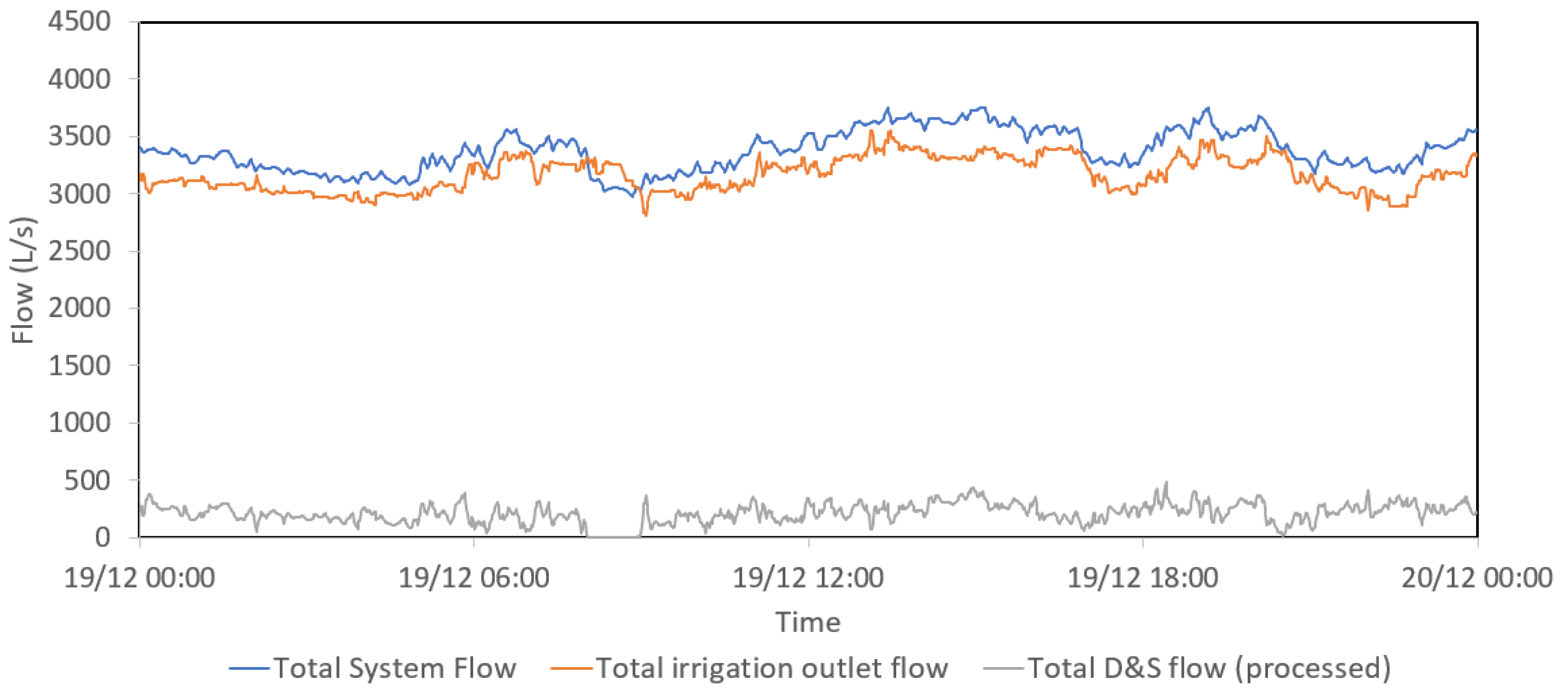
Similarly, the flow data for each demand category during the model validation period has been obtained and processed, as summarized in Figure 4 below.

3.4. Model Calibration

3.4.1. Calibration Process

The proposed calibration process in Figure 1 above has been applied to the case study system. First, for the model simplification, pipes with roughness values that can impact the pressures at the five monitoring sites (RTU 1 to 5 in Figure 2 above) are selected to form the pruned network. For instance, pipes downstream of RTU 4 will not be selected for calibration as their roughness values will not have an impact on the pressure readings of this sensor. The original network with 433 pipes has been then simplified to a pruned network with 126 pipes. Second, the optimization objective for this system becomes the minimization of the average of the five RMSE values between the measured and the predicted pressures with timesteps of 1 min at the five pressure monitoring sites.

3.4.2. Decision Variable Set Formulations

For the four different formulations for defining decision variables (DVs), 126 DVs, 4 DVs, 10 DVs and 34 DVs have been identified (see Section 2.4), respectively. In Formulation 1, each pipe roughness value of the 126 pipes in the pruned network is regarded as a decision variable. In Formulation 2, the pipe roughness values of 4 pipe materials are regarded as 4 decision variables. In Formulation 3, there are 10 different combinations of materials and diameters, which form the 10 decision variables. To identify decision variables for Formulation 4, five design demand patterns were used to simulate the potential maximum pipe flows based on LMW operational rules and the system delivery capacity. The average velocity of each pipe under the five demand patterns was used.

4. Results and Discussion

In this section, results from the three optimization methods and the four different ways of defining decision variables are presented and compared. The optimization results are then compared to the results obtained with pipe roughness values commonly used in engineering practice. The calibrated model was then validated using independent data.

4.1. Model Calibration Results

4.1.1. Optimization Settings for Model Calibration

A total of 10 runs with different random seeds have been conducted for each combination of the three optimization methods and four decision variable set formulations (i.e., in total 120 optimization runs were conducted). In order to make a fair comparison of results between different optimization methods, the same stopping (convergence) criterion was applied to the three methods. In this paper, the objective function tolerance f _ t o l [70] which represents the precision goal of objective function values has been selected as the stopping (convergence) criterion. When | f ( x i ) f ( x i + 1 ) | < f t o l = 10 6 , the objective function is regarded as converged in each of the three optimization methods. The inequality constraints for all methods and decision variable set formulations are set to be the lower and upper bound of 0.01 mm and 20 mm, respectively, of potential pipe roughness height values. The upper bound is much larger than common roughness values used in urban water supply systems which deliver treated clean water. This is because the case study system delivers untreated raw water from the Murray River, so that significantly larger pipe roughness values may occur over time considering the potential impact of biofilm growth [52,71].
Besides the constraints, another input parameter for the SLSQP is the initial guess vector x 0 for the decision variables. A random number generator has been used to generate the initial x 0 values within the given bounds (0.01, 20) mm for each run. For the GA and DE, random seeds have also been used to specify the starting point of the initial population in the search space. Other key parameters selected for the GA and DE are listed in Table 2. These parameters include the population size ( N ) for both, the probability of crossover ( p c ) and the probability of mutation ( p m ) for the GA, as well as the crossover rate ( C R ) and the weighting factor ( F ) for the DE. For the GA, a series of sensitivity analyses were conducted for choosing these parameter values. For the DE, the most common initial settings have been chosen as suggested in the literature [72,73,74]. In addition, a parameter control technique ‘dither’ [75] has been adopted for the DE in pymoo where F is selected from the interval (0.5, 1.0) randomly for each individual vector [76]. This can significantly improve convergence behavior.
In Section 4.1.1, results obtained from each of the optimization methods and formulations are compared. Results (the objective function value) obtained from using common pipe roughness values in engineering practice are also compared with results obtained using optimization methods. In Section 4.1.2, a detailed comparison between field-observed and model-predicted values at each of the monitoring sites is presented.

4.1.2. Model Calibration Results

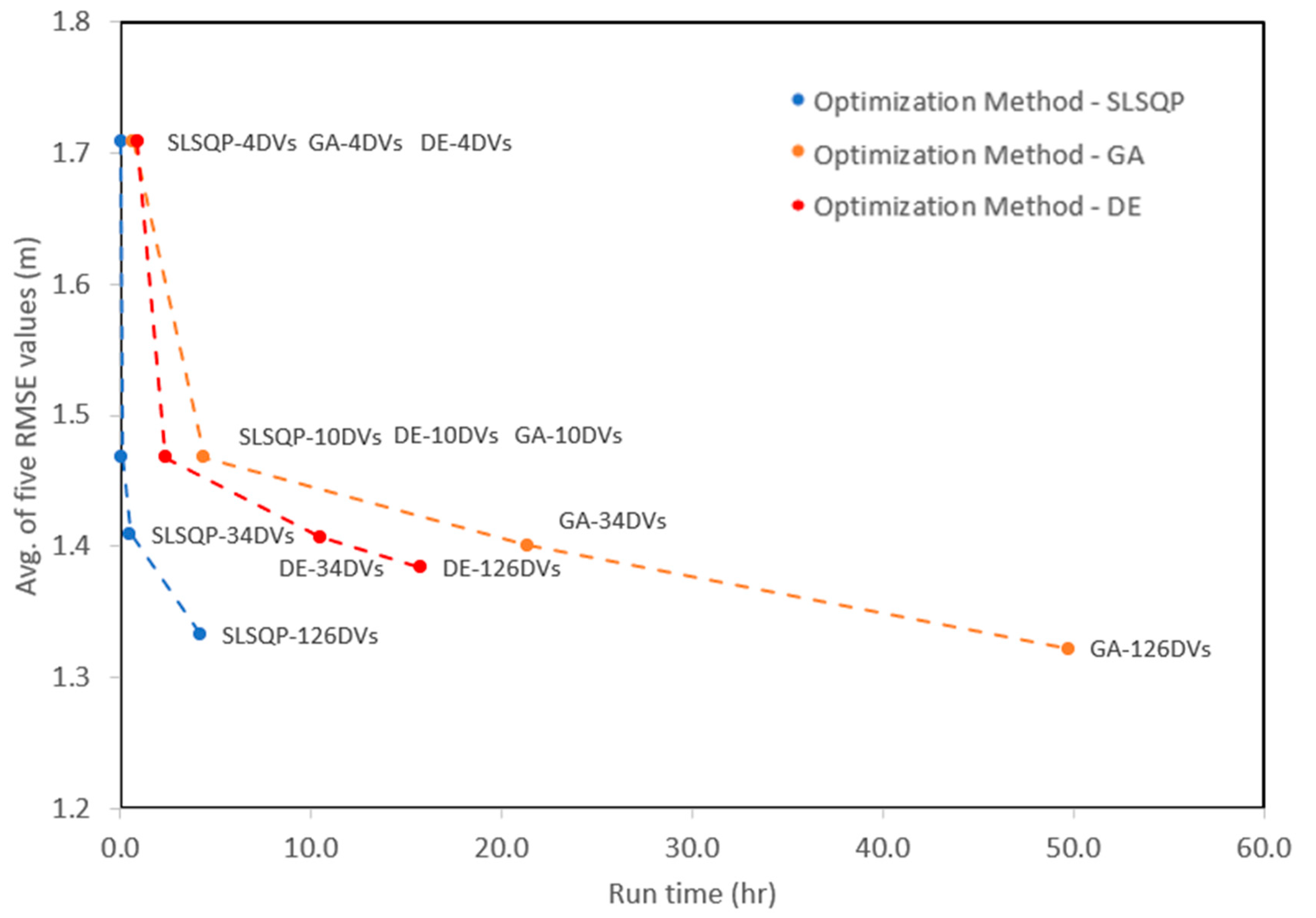
The optimization results of the average values of the 10 runs (each with a different starting random seed) for each optimization method and decision variable set formulation are summarized in Table 3. The average of the objective function values and run times of the 10 runs are also plotted in Figure 5. In addition, the average number of generations (iterations for SLSQP) and evaluations required for the 10 runs are also given in Table 3. Full results of the 10 runs have been provided in Tables S1 and S2 in the Supplementary Material.
As shown in Figure 5, for each optimization method, trade-offs between the objective function values and the run time are evident. The increase in run time can lead to a decrease in objective function values. For the same optimization method, the objective function value decreases with an increase in the number of decision variables. For instance, for the GA method, the average of the 10 runs of the average of the five RMSE values decreases from about 1.709 m to 1.322 m with an increase in the number of decision variables from 4 to 126 (i.e., the average of RMSE values: 4 DVs > 10 DVs > 34 DVs > 126 DVs). In addition, for the same optimization method, the run time increases significantly with an increase in the number of decision variables. For example, also for the GA method, the run time increases from about 0.55 h to 33.9 h with an increase in the number of decision variables from 4 to 126 (i.e., run time: 4 DVs < 10 DVs < 34 DVs < 126 DVs).
For all three optimization methods, as shown in Figure 5, the average objective function values for Formulation 2 (4 DVs) are the largest out of all decision variable set formulations, which is followed by Formulation 3 (10 DVs) and Formulation 4 (34 DVs). The average objective function values in Formulation 1 (126 DVs) are the smallest in comparison with the other decision variable set formulations. Under the same decision variable set formulation, very close objective function values are evident for all three optimization methods, particularly in Formulation 2 (4 DVs), Formulation 3 (10 DVs) and Formulation 4 (34 DVs). However, in Formulation 1 (126 DVs), DE results in a slightly larger objective function value (about 1.384 m). In addition, under the same decision variable set formulation, SLSQP always takes the least run time in comparison with the other two optimization methods. In Formulation 2 (4 DVs), DE requires slightly more run time than the other two methods. Nevertheless, in the other three decision variable set formulations, the GA takes the longest, followed by DE and then SLSQP.
Results (the objective function values) obtained using the optimization methods have also been compared to common values likely to be selected based on engineering judgment in real-world practice. The common pipe roughness height values are taken as 0.15, 0.06, 0.06 and 0.015 mm for MSCL, DICL, GRP and mPVC pipes, respectively [77]. The objective function value is calculated to be 4.099 m after applying these values to the case study system. It is evident that the average of the five RMSE values is much larger than any of the results obtained from using optimization methods.

4.2. Discussion of Model Calibration Results

Different pipe roughness values have been obtained from different decision variable set formulations. In terms of a general trend, for Formulations 2 (4 DVs), large roughness values, particularly for MSCL and GRP pipes, were obtained. For the other three decision variable set formulations with higher numbers of decision variables, some unrealistic combinations of pipe roughness values were obtained, despite limited improvement in the objective function values. For further analysis, pipe roughness values obtained from Formulations 2 (4 DVs) and Formulations 3 (10 DVs) are shown in Table 4 and Table 5, respectively.
As shown in Table 4, large roughness values, particularly for MSCL and GRP pipes, have been obtained using Formulation 2 with 4 DVs. This is a reasonable result, although was unexpected initially. The system has been used to pump raw water from the River Murray, there can potentially be significant growth of biofilms in pipes in the past ten years. Biofilms are complex microbiological slime layers that aggregate microorganisms in a polymer matrix [53,78]. They predominantly occur in raw or recycled water systems that deliver water containing a high level of nutrients such as dissolved organic carbon (DOC) in particular [52,53]. The Robinvale irrigation system carries raw water pumped from the Murray River, which forms the environment for the growth of biofilms in pipes. The major hydraulic impact imposed by biofilms is a dramatic increase in friction head loss [71,78,79], as the roughness height values of pipes can increase significantly over time [52,71]. For example, according to the results from a laboratory experiment [52], the roughness height value increased from approximately 0.01 mm to about 6.8 mm in a relatively short period (about 400 h).
When the number of decision variables is increased, for Formulation 3 with 10 DVs, for example, it has been found that some unrealistic combinations of pipe roughness values were obtained, as shown in Table 5. For instance, for DV1 and DV2 which have the same pipe material (mPVC) in Table 5, a small change in the diameter from 300 to 375 mm leads to significantly different pipe roughness values of 0.01 and 20 mm, respectively. In fact, the roughness values of these mPVC pipes have a limited impact on the pressure sensor readings. The algorithm tries to achieve a very slight improvement in the objective function values by pushing the two roughness values to the two extreme ends (lower and upper bounds). Hence, it is important to use engineering judgment to modify any anomalous calibrated pipe roughness values that are the outcome of the optimization process.
The reason behind this is related to the fitness landscape [33] of the optimization problem and the different levels of complexity resulting from different decision variable formulations. The finer resolutions of the fitness landscape resulting from more decision variables can potentially lead the search into local numerical optimums, which may not have realistic pipe roughness values. In addition, the finer resolution of the fitness landscape has a higher chance of leading to the phenomenon of equifinality [80,81], which refers to that the same objective function value can be achieved by different combinations of decision variables. This can also lead to unrealistic combinations of solutions with a slight improvement in objective function values. For instance, the percentage of the average error increases only about 0.5% when the number of decision variables increases from 4 to 126, at a cost of generating a large number of unrealistic combinations of solutions with a much longer run time. Additionally, the insignificant improvement in the relative error can be much smaller than the system or measurement errors, which can be 5% to 10% depending on the system. Therefore, for this case study, the formulation of 4 decision variables is sufficient to achieve a good level of calibration in a shorter run time without creating unrealistic combinations of pipe roughness values. This finding is further confirmed by the results obtained for Formulation 4 with 34 DVs and Formulation 1 with 126 DVs.
There are some insights obtained from the results and analysis above: (1) the use of optimization methods has added value to the model calibration by making much better results in comparison with that using common engineering practice (e.g., the objective function has been decreased from around 4 m to less than 1.8 m); (2) the more complicated (or the finer) problem formulations or the more advanced methods do not necessarily lead to better results; and (3) when similar results (e.g., objective function values) are obtained from different methods (e.g., decision variable formulation or optimization algorithm), a simpler method should be selected. For the case of this study, Formulation 2 with 4 DVs and the SLSQP optimization method is the best combination for pipe roughness calibration. The results obtained from this combination of decision variable formulation and optimization method are further evaluated using both calibration and validation data below.
Nevertheless, there are still limitations and room for improvement associated with this study. First, the proposed methods and decision variable set formulations have been tested on only one real-world network, and their application to other systems (e.g., networks with more complex loops) needs to be investigated in future research to see if similar conclusions can be drawn. In addition, further exploration of the mathematical model for different decision variable set formulations can be considered in future research to better understand the generation of unrealistic combinations of solutions with the increase in the number of decision variables. Finally, in this study, the model is calibrated based on pressure data while the demand is assumed to be fixed. The feasibility of the proposed methods and decision variable set formulations can be further investigated in future research when calibrating the demands and pressures at the same time.
In addition, optimized pipe roughness values obtained from Formulation 2 (4 DVs with the SLSQP method) have been selected as input into the hydraulic model to calculate the model-simulated results which are to be compared with field observations. The minimum average of the five RMSE values from the five pressure sensor locations is calculated to be 1.709 m. The field-observed HGL versus the model-predicted values at two pressure monitoring sites (RTU 1 and RTU 5) as two examples are shown in Figure 6 below. In general, a good match between the modeled and the observed values of each site has been achieved. Full results of the breakdown and comparison of the measured and modeled values at each monitoring site are provided in Table S3 and Figure S1 in the Supplementary Material.

4.3. Evaluation of Formulation 2 (4 DVs) Using Validation Data

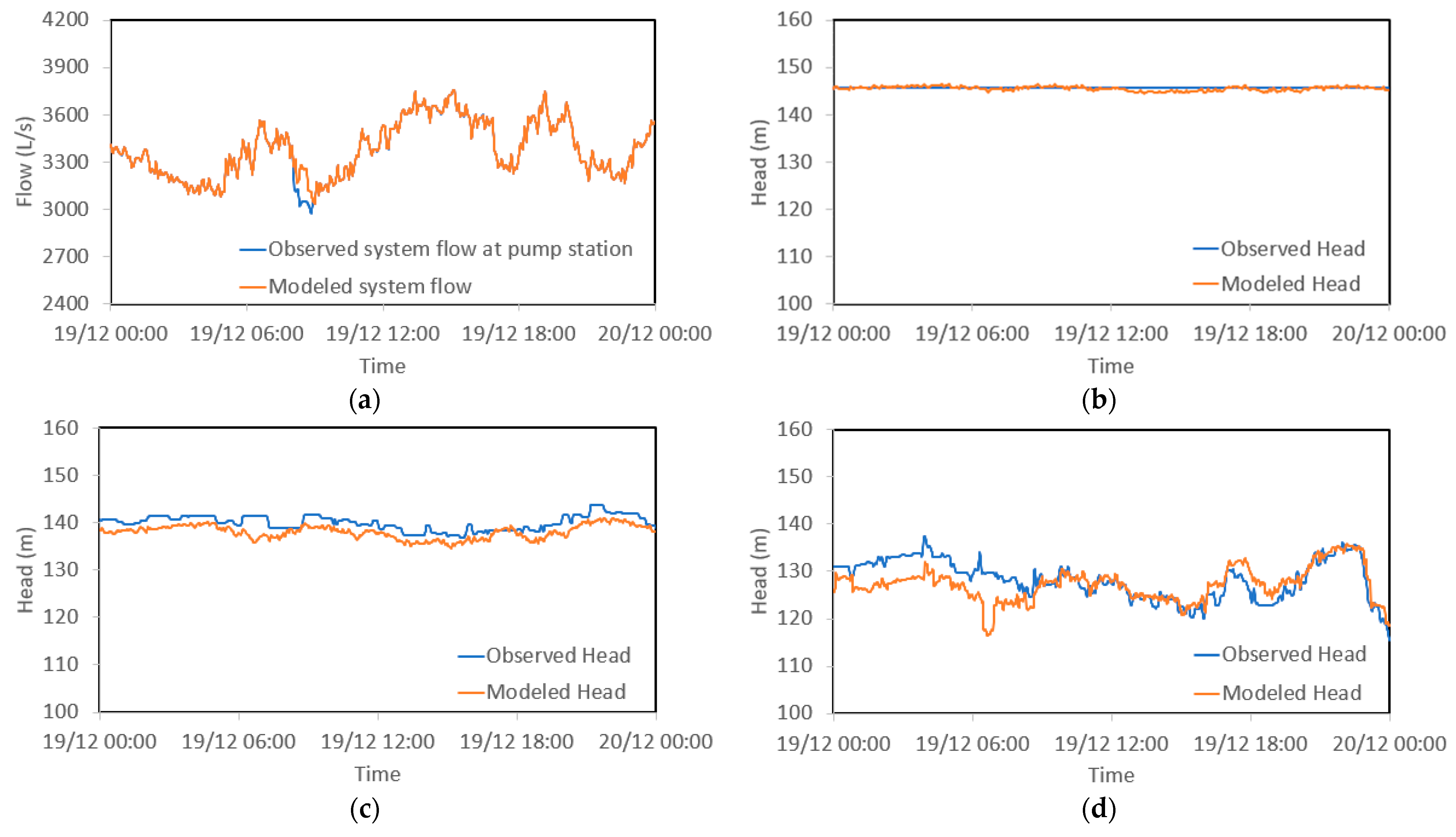
The breakdown of the average observed and modeled values, percentages, as well as the individual RMSE value at each monitoring site during the validation period, is summarized in Table 6. In this case, all the average differences between the modeled and observed HGL are less than 1.5 m [9], which indicates a satisfactory level of validation has been achieved.
The field-observed HGL and flows versus the model-predicted values at each pressure monitoring site are shown in Figure 7 below. In general, a good match between the modeled and the observed values of each site has been achieved. It has been noticed that there is an evident mismatch between modeled and the observed HGL values before 10 a.m. for RTU3. This can be potentially caused by anomalies (or equipment errors) that occurred in the measurement process of pressures during this period.

5. Summary and Conclusions

In this paper, three different optimization methods for hydraulic model calibration are compared. These methods include Sequential Least Squares Programming (SLSQP), a Genetic Algorithm (GA) and Differential Evolution (DE). Their performance is investigated over four different decision variable set formulations, where different numbers of decision variables are used to represent different levels of discretization of the search space. A real-world pressurized irrigation system in Victoria, Australia has been selected as the case study system.
It has been found that first for the same optimization method, an increase in the number of decision variables can lead to a slight decrease in objective function values but with a corresponding significant increase in run time. Second, for the same decision variable set formulation, similar objective function values are evident for all three optimization methods. SLSQP always takes the least run time in comparison with the other two methods. In most cases, GA takes the longest run time, which is followed by DE. It can be inferred that the objective function search space of this problem is relatively flat as both local and global algorithms have converged for all three optimization methods and four decision variable set formulations. Furthermore, different pipe roughness values have been obtained from different decision variable set formulations. The increase in the number of decision variables has led to some unrealistic combinations of pipe roughness values obtained, despite limited improvement in the objective function values.
It is evident from the results obtained that formal optimization does improve WDS hydraulic model calibration compared to setting pipe roughness values based on common engineering judgment. The different ways to formulate the decision variable have a slight impact on the performance of optimized solutions in terms of objective function values, with more complicated formulation leading to slightly improved results. However, the finer problem formulation does not necessarily lead to feasible solutions. A simpler formulation that suits the case study system and the data available can be better. Further, different combinations of decision variable formulations and optimization algorithms can lead to very similar results. In this case, a simpler method is often better. Finally, in this study, some large pipe roughness values have been obtained. This is very likely due to the significant growth of biofilms in pipes in the past ten years, as the network supplies raw river water that contains essential nutrients for excessive biofilm growth. Therefore, biofilm growth should be a consideration in WDS hydraulic model calibration, particularly for systems delivering untreated water.
There are also some issues that can be considered in future research. First, the proposed methods and decision variable set formulations should be tested for other case study systems, including networks with more complex loops. This would provide general guidelines for the selection of a suitable combination of optimization algorithms and decision variable set formulations for the WDS model calibration. In addition, further exploration of the mathematical model for different decision variable set formulations could be considered in future research to better understand the generation of unrealistic combinations of solutions with an increase in the number of decision variables.

Supplementary Materials

The following supporting information can be downloaded at: https://www.mdpi.com/article/10.3390/w14203276/s1, Figure S1: (a) Comparison of the observed and modeled system total flow during the calibration period; (b–f): Comparison of the observed and modeled HGL at RTU1 to RTU5 during the calibration period; Table S1: Full optimization results obtained from three optimization methods and four decision variable set formulations; Table S2: The number of generations and evaluations required for all runs; Table S3: Observed and simulated pressure data over the calibration period at each monitoring site.

Author Contributions

Conceptualization, Q.Z., W.W. and A.R.S.; methodology, Q.Z., W.W. and A.R.S.; software, Q.Z.; validation, Q.Z., W.W., A.R.S. and A.W.; formal analysis, Q.Z., W.W. and A.R.S.; investigation, Q.Z.; resources, A.W.; data curation, A.W.; writing—original draft preparation, Q.Z.; writing—review and editing, Q.Z., W.W., A.R.S. and A.W.; visualization, Q.Z. and W.W.; supervision, W.W., A.R.S. and A.W.; project administration, Q.Z. All authors have read and agreed to the published version of the manuscript.

Funding

Wenyan Wu acknowledges financial support from the Australian Research Council via the Discovery Early Career Researcher Award (DE210100117).

Data Availability Statement

Data available on request due to restrictions (subject to Lower Murray Water’s approval).

Acknowledgments

We would like to thank Lower Murray Water for supplying data for this paper. Wenyan Wu acknowledges support from the Australian Research Council via the Discovery Early Career Researcher Award (DE210100117). This research is supported by The University of Melbourne’s Research Computing Services and the Petascale Campus Initiative.

Conflicts of Interest

The authors declare no conflict of interest.

References

  1. Mendez, M.; Araya, J.A.; Sanchez, L.D. Automated parameter optimization of a water distribution system. J. Hydroinform. 2013, 15, 71–85. [Google Scholar] [CrossRef]
  2. Zhang, Q.; Zheng, F.; Duan, H.-F.; Jia, Y.; Zhang, T.; Guo, X. Efficient numerical approach for simultaneous calibration of pipe roughness coefficients and nodal demands for water distribution systems. J. Water Resour. Plan. Manag. 2018, 144, 04018063. [Google Scholar] [CrossRef]
  3. Wu, Z.Y.; Walski, T.M.; Mankowski, R.; Herrin, G.; Gurierri, R.; Tryby, M. Calibrating water distribution model via genetic algorithms. In Proceedings of the AWWA Information Management and Technology Conference, Kansas City, MO, USA, 14–17 April 2002. [Google Scholar]
  4. Savic, D.A.; Kapelan, Z.S.; Jonkergouw, P.M.R. Quo vadis water distribution model calibration? Urban Water J. 2009, 6, 3–22. [Google Scholar] [CrossRef]
  5. Walski, T.M.; DeFrank, N.; Voglino, T.; Wood, R.; Whitman, B.E. Determining the accuracy of automated calibration of pipe network models. In Proceedings of the Eighth Annual Water Distribution Systems Analysis Symposium, Cincinnati, OH, USA, 27–30 August 2006. [Google Scholar]
  6. Ormsbee, L.E.; Wood, D.J. Explicit pipe network calibration. J. Water Resour. Plan. Manag. 1986, 112, 166–182. [Google Scholar] [CrossRef]
  7. Shamir, U.Y.; Howard, C.D.D. Water distribution systems analysis. J. Hydraul. Div. 1968, 94, 219–234. [Google Scholar] [CrossRef]
  8. Gao, T. Pipe roughness estimation in water distribution networks using head loss adjustment. J. Water Resour. Plan. Manag. 2017, 143, 04017007. [Google Scholar] [CrossRef]
  9. Walski, T.M. Technique for calibrating network models. J. Water Resour. Plan. Manag. 1983, 109, 360–372. [Google Scholar] [CrossRef]
  10. Walski, T.M. Case-study—Pipe network model calibration issues. J. Water Resour. Plan. Manag. 1986, 112, 238–249. [Google Scholar] [CrossRef]
  11. Hutton, C.J.; Kapelan, Z.; Vamvakeridou-Lyroudia, L.; Savic, D.A. Dealing with uncertainty in water distribution system models: A framework for real-time modeling and data assimilation. J. Water Resour. Plan. Manag. 2014, 140, 169–183. [Google Scholar] [CrossRef]
  12. Maier, H.R.; Ascough Ii, J.C.; Wattenbach, M.; Renschler, C.S.; Labiosa, W.B.; Ravalico, J.K. Chapter five uncertainty in environmental decision making: Issues, challenges and future directions. In Developments in Integrated Environmental Assessment; Jakeman, A.J., Voinov, A.A., Rizzoli, A.E., Chen, S.H., Eds.; Elsevier: Amsterdam, The Netherlands, 2008; Volume 3, pp. 69–85. [Google Scholar]
  13. Walski, T.M.; Chase, D.V.; Savic, D.A. Water Distribution Modeling; Haestad Press: Waterbury, CT, USA, 2001. [Google Scholar]
  14. Walski, T.M.; Chase, D.V.; Savic, D.A.; Grayman, W.; Beckwith, S.; Koelle, E. Advanced Water Distribution Modeling and Management; Haestad Press: Waterbury, CT, USA, 2003. [Google Scholar]
  15. Ostfeld, A.; Salomons, E.; Ormsbee, L.; Uber, J.G.; Bros, C.M.; Kalungi, P.; Burd, R.; Zazula-Coetzee, B.; Belrain, T.; Kang, D. Battle of the water calibration networks. J. Water Resour. Plan. Manag. 2012, 138, 523–532. [Google Scholar] [CrossRef]
  16. Do, N.C.; Simpson, A.R.; Deuerlein, J.W.; Piller, O. Calibration of water demand multipliers in water distribution systems using genetic algorithms. J. Water Resour. Plan. Manag. 2016, 142, 04016044. [Google Scholar] [CrossRef]
  17. Kang, D.; Lansey, K. Demand and roughness estimation in water distribution systems. J. Water Resour. Plan. Manag. 2011, 137, 20–30. [Google Scholar] [CrossRef]
  18. Kapelan, Z. Calibration of Water Distribution System Hydraulic Models. Ph.D. Thesis, University of Exeter, Exeter, UK, 2002. [Google Scholar]
  19. Rahal, C.M.; Sterling, M.J.H.; Coulbeck, B. Parameter tuning for simulation-models of water distribution networks. Proc. Inst. Civ. Eng. 1980, 69 Pt 2, 751–762. [Google Scholar] [CrossRef]
  20. Bhave, P.R. Calibrating water distribution network models. J. Environ. Eng. 1988, 114, 120–136. [Google Scholar] [CrossRef]
  21. Lansey, K.E.; Basnet, C. Parameter-estimation for water distribution networks. J. Water Resour. Plan. Manag. 1991, 117, 126–144. [Google Scholar] [CrossRef]
  22. Boulos, P.F.; Ormsbee, L.E. Explicit network calibration for multiple loading conditions. Civ. Eng. Syst. 1991, 8, 153–160. [Google Scholar] [CrossRef]
  23. Boulos, P.F.; Wood, D.J. Explicit calculation of pipe-network parameters. J. Hydraul. Eng. 1990, 116, 1329–1344. [Google Scholar] [CrossRef]
  24. Ferreri, G.B.; Napoli, E.; Tumbiolo, A. Calibration of roughness in water distribution networks. In Proceedings of the 2nd International Conference on Water Pipeline System, Edinburgh, UK, 24–26 May 1994. [Google Scholar]
  25. Andersen, J.H.; Powell, R.S. Implicit state-estimation technique for water network monitoring. Urban Water 2000, 2, 123–130. [Google Scholar] [CrossRef]
  26. Hutton, C.J.; Kapelan, Z.; Vamvakeridou-Lyroudia, L.; Savic, D.A. Real-time demand estimation in water distrubtion systems under uncertainty. In Proceedings of the WDSA 2012: 14th Water Distribution Systems Analysis Conference, Adelaide, SA, Australia, 24–27 September 2012. [Google Scholar]
  27. Kang, D.; Lansey, K. Real-time demand estimation and confidence limit analysis for water distribution systems. J. Hydraul. Eng. 2009, 135, 825–837. [Google Scholar] [CrossRef]
  28. Ormsbee, L.E. Implicit network calibration. J. Water Resour. Plan. Manag. 1989, 115, 243–257. [Google Scholar] [CrossRef]
  29. Ormsbee, L.E.; Lingireddy, S. Calibrating hydraulic network models. J. Am. Water Work. Assoc. 1997, 89, 42–50. [Google Scholar] [CrossRef]
  30. Savic, D.A.; Walters, G.A. Genetic Algorithm Techniques for Calibrating Network Models; University of Exeter: Exeter, UK, 1995. [Google Scholar]
  31. Shang, F.; Uber, J.G.; van Bloemen Waanders, B.G.; Boccelli, D.; Janke, R. Real time water demand estimation in water distribution system. In Proceedings of the Water Distribution Systems Analysis Symposium, Kruger National Park, South Africa, 17–20 August 2008. [Google Scholar]
  32. Walski, T.; Wu, Z.; Hartell, W. Performance of automated calibration for water distribution systems. In Critical Transitions in Water and Environmental Resources Management; Amer Society of Civil Engineers: Reston, VA, USA, 2004; pp. 1–10. [Google Scholar]
  33. Maier, H.R.; Razavi, S.; Kapelan, Z.; Matott, L.S.; Kasprzyk, J.; Tolson, B.A. Introductory overview: Optimization using evolutionary algorithms and other metaheuristics. Environ. Model. Softw. 2019, 114, 195–213. [Google Scholar] [CrossRef]
  34. Bagloee, S.A.; Asadi, M.; Patriksson, M. Minimization of water pumps’ electricity usage: A hybrid approach of regression models with optimization. Expert Syst. Appl. 2018, 107, 222–242. [Google Scholar] [CrossRef]
  35. Coelho, B.; Andrade-Campos, A. Efficiency achievement in water supply systems—A review. Renew. Sustain. Energy Rev. 2014, 30, 59–84. [Google Scholar] [CrossRef]
  36. Abkenar, S.M.S.; Stanley, S.D.; Miller, C.J.; Chase, D.V.; McElmurry, S.P. Evaluation of genetic algorithms using discrete and continuous methods for pump optimization of water distribution systems. Sustain. Comput. Inform. Syst. 2015, 8, 18–23. [Google Scholar]
  37. Shamir, U. Optimal design and operation of water distribution systems. Water Resour. Res. 1974, 10, 27–36. [Google Scholar] [CrossRef]
  38. Datta, R.S.N.; Sridharan, K. Parameter-estimation in water-distribution systems by least-squares. J. Water Resour. Plan. Manag. 1994, 120, 405–422. [Google Scholar] [CrossRef]
  39. Reddy, P.V.N.; Sridharan, K.; Rao, P.V. Wls method for parameter estimation in water distribution networks. J. Water Resour. Plan. Manag. 1996, 122, 157–164. [Google Scholar] [CrossRef]
  40. Press, W.H.; William, H.; Teukolsky, S.A.; Vetterling, W.T.; Saul, A.; Flannery, B.P. Numerical Recipes 3rd Edition: The Art of Scientific Computing; Cambridge University Press: Cambridge, UK, 2007. [Google Scholar]
  41. Creaco, E.; Pezzinga, G. Embedding linear programming in multi objective genetic algorithms for reducing the size of the search space with application to leakage minimization in water distribution networks. Environ. Model. Softw. 2015, 69, 308–318. [Google Scholar] [CrossRef]
  42. Maier, H.R.; Kapelan, Z.; Kasprzyk, J.; Kollat, J.; Matott, L.S.; Cunha, M.C.; Dandy, G.C.; Gibbs, M.S.; Keedwell, E.; Marchi, A.; et al. Evolutionary algorithms and other metaheuristics in water resources: Current status, research challenges and future directions. Environ. Model. Softw. 2014, 62, 271–299. [Google Scholar] [CrossRef] [Green Version]
  43. Coelho, B.; Andrade-Campos, A. Using different strategies for improving efficiency in water supply systems. In Proceedings of the 1st ECCOMAS Young Investigators Conference, Aveiro, Portugal, 24–27 April 2012. [Google Scholar]
  44. Zecchin, A.C.; Maier, H.R.; Simpson, A.R.; Leonard, M.; Nixon, J.B. Ant colony optimization applied to water distribution system design: Comparative study of five algorithms. J. Water Resour. Plan. Manag. 2007, 133, 87–92. [Google Scholar] [CrossRef]
  45. Wolpert, D.H.; Macready, W.G. No free lunch theorems for optimization. IEEE Trans. Evol. Comput. 1997, 1, 67–82. [Google Scholar] [CrossRef] [Green Version]
  46. Letting, L.K.; Hamam, Y.; Abu-Mahfouz, A.M. Estimation of water demand in water distribution systems using particle swarm optimization. Water 2017, 9, 593. [Google Scholar] [CrossRef] [Green Version]
  47. Zanfei, A.; Menapace, A.; Santopietro, S.; Righetti, M. Calibration procedure for water distribution systems: Comparison among hydraulic models. Water 2020, 12, 1421. [Google Scholar] [CrossRef]
  48. Minaee, R.P.; Afsharnia, M.; Moghaddam, A.; Ebrahimi, A.A.; Askarishahi, M.; Mokhtari, M. Calibration of water quality model for distribution networks using genetic algorithm, particle swarm optimization, and hybrid methods. MethodsX 2019, 6, 540–548. [Google Scholar] [CrossRef]
  49. Roma, J.; Perez, R.; Sanz, G.; Grau, S. Model calibration and leakage assessment applied to a real water distribution network. Procedia Eng. 2015, 119, 603–612. [Google Scholar] [CrossRef] [Green Version]
  50. Walters, G.; Savic, D.; Morley, M.; De Schaetzen, W.; Atkinson, R. Calibration of water distribution network models using genetic algorithms. WIT Trans. Ecol. Environ. 1998, 26, 131–140. [Google Scholar]
  51. Gong, J.; Erkelens, M.; Lambert, M.F.; Forward, P. Experimental study of dynamic effects of iron bacteria–formed biofilms on pipeline head loss and roughness. J. Water Resour. Plan. Manag. 2019, 145, 04019038. [Google Scholar] [CrossRef]
  52. Lambert, M.F.; Brookes, J.; Kildea, M.; Grantham, T.; McFarlane, B. Understanding the impact of biofilm growth on pipe roughness. In Proceedings of the World Environmental and Water Resources Congress 2008, Honolulu, HI, USA, 12–16 May 2008. [Google Scholar]
  53. Lambert, M.F.; Edwards, R.W.J.; Howie, S.J.; De Gilio, B.B.; Quinn, S.P. The impact of biofilm development on pipe roughness and velocity profile. In Proceedings of the World Environmental and Water Resources Congress 2009, Kansas City, MO, USA, 17–21 May 2009. [Google Scholar]
  54. Kraft, D. A Software Package for Sequential Quadratic Programming; DFVLR Obersfaffeuhofen: Weßling, Germany, 1988. [Google Scholar]
  55. Golberg, D.E. Genetic algorithms in search, optimization, and machine learning. Addion Wesley 1989, 1989, 36. [Google Scholar]
  56. Storn, R.; Price, K. Differential evolution–a simple and efficient heuristic for global optimization over continuous spaces. J. Glob. Optim. 1997, 11, 341–359. [Google Scholar] [CrossRef]
  57. Ahmad, M.F.; Isa, N.A.M.; Lim, W.H.; Ang, K.M. Differential evolution: A recent review based on state-of-the-art works. Alex. Eng. J. 2021, 61, 3831–3872. [Google Scholar] [CrossRef]
  58. Kachitvichyanukul, V. Comparison of three evolutionary algorithms: Ga, pso, and de. Ind. Eng. Manag. Syst. 2012, 11, 215–223. [Google Scholar] [CrossRef] [Green Version]
  59. Liu, J.; Lampinen, J. A fuzzy adaptive differential evolution algorithm. Soft Comput. 2005, 9, 448–462. [Google Scholar] [CrossRef]
  60. Blank, J.; Deb, K. Pymoo: Multi-objective optimization in python. IEEE Access 2020, 8, 89497–89509. [Google Scholar] [CrossRef]
  61. Open Water Analytics. Owa-Epanet 2.2.4; Open Water Analytics: Andover, MA, USA, 2020. Available online: https://community.wateranalytics.org/ (accessed on 4 July 2022).
  62. Rossman, L. The Epanet Programmer’s Toolkit; National Risk Management Research Laboratory, Office of Research and Development, U.S. Environmental Protection Agency: Cincinnati, OH, USA, 1999.
  63. Walski, T. Procedure for hydraulic model calibration. J. Am. Water Work. Assoc. 2017, 109, 55–61. [Google Scholar] [CrossRef]
  64. Lower Murray Water. Lower Murray Water Annual Report 2018–2019; Lower Murray Water: Mildura, VIC, Australia, 2019.
  65. Lower Murray Water. Lower Murray Water Corporate Plan 2019–2020; Lower Murray Water: Mildura, VIC, Australia, 2019.
  66. Google Maps. Victoria, Australia; Google Maps: Mountain View, CA, USA, 2022; Available online: https://www.google.com/maps/place/%E7%B6%AD%E5%A4%9A%E5%88%A9%E4%BA%9E%E7%9C%81/@-36.5052093,140.9779493,6z/data=!3m1!4b1!4m5!3m4!1s0x6ad4314b7e18954f:0x5a4efce2be829534!8m2!3d-36.9847807!4d143.3906074 (accessed on 4 July 2022).
  67. Walski, T.M. Model calibration data: The good, the bad, and the useless. J. Am. Water Work. Assoc. 2000, 92, 94–99. [Google Scholar] [CrossRef]
  68. Pietrucha-Urbanik, K.; Studzinski, A. Selected issues of costs and failure of pipes in an exemplary water supply system. Rocz. Ochr. Srodowiska 2016, 18, 616–627. [Google Scholar]
  69. Studziński, A.; Pietrucha-Urbanik, K. Failure risk analysis of water distributions systems using hydraulic models on real field data. Ekon. Sr. 2019, 68, 152–165. [Google Scholar]
  70. Blank, J.; Deb, K. Termination Criterion. Available online: https://pymoo.org/interface/termination.html (accessed on 4 July 2022).
  71. Picologlou, B.F.; Characklis, W.G.; Zelver, N. Biofilm growth and hydraulic performance. J. Hydraul. Div. 1980, 106, 733–746. [Google Scholar] [CrossRef]
  72. Centeno-Telleria, M.; Zulueta, E.; Fernandez-Gamiz, U.; Teso-Fz-Betoño, D.; Teso-Fz-Betoño, A. Differential evolution optimal parameters tuning with artificial neural network. Mathematics 2021, 9, 427. [Google Scholar] [CrossRef]
  73. Ronkkonen, J.; Kukkonen, S.; Price, K.V. Real-parameter optimization with differential evolution. In Proceedings of the IEEE Congress on Evolutionary Computation, Edinburgh, UK, 2–5 September 2005. [Google Scholar]
  74. Storn, R. On the usage of differential evolution for function optimization. In Proceedings of the North American Fuzzy Information Processing, Berkeley, CA, USA, 19 June 1996. [Google Scholar]
  75. Dawar, D.; Ludwig, S.A. Differential evolution with dither and annealed scale factor. In Proceedings of the 2014 IEEE Symposium on Differential Evolution (SDE), Orlando, FL, USA, 9–12 December 2014. [Google Scholar]
  76. Blank, J.; Deb, K. De: Differential Evolution. Available online: https://pymoo.org/algorithms/soo/de.html#DE:-Differential-Evolution (accessed on 4 July 2022).
  77. Standards Australia. AS 2200: 2006; Design Charts for Water Supply and Sewerage. Standards Australia: Sydney, NSW, Australia, 2006.
  78. Cowle, M.W.; Babatunde, A.O.; Rauen, W.B.; Bockelmann-Evans, B.N.; Barton, A.F. Biofilm development in water distribution and drainage systems: Dynamics and implications for hydraulic efficiency. Environ. Technol. Rev. 2014, 3, 31–47. [Google Scholar] [CrossRef]
  79. Characklis, W.G. Attached microbial growths-ii. Frictional resistance due to microbial slimes. Water Res. 1973, 7, 1249–1258. [Google Scholar] [CrossRef] [Green Version]
  80. Beven, K. Prophecy, reality and uncertainty in distributed hydrological modeling. Adv. Water Resour. 1993, 16, 41–51. [Google Scholar] [CrossRef]
  81. Beven, K. A manifesto for the equifinality thesis. J. Hydrol. 2006, 320, 18–36. [Google Scholar] [CrossRef]
Figure 1. Calibration process in this study.
Water 14 03276 g001
Figure 2. Case study system (the location of the system was generated with Google Maps [66], and the layout of the network was provided by LMW).
Water 14 03276 g002
Figure 3. Total flow of each demand category during the calibration period.
Water 14 03276 g003
Figure 4. Total flow of each demand category during the validation period.
Water 14 03276 g004
Figure 5. Optimization results—4 different decision variable set formulations under 3 optimization methods.
Water 14 03276 g005
Figure 6. Comparison of the observed and modeled HGL at: (a) RTU1; (b) RTU5 during the calibration period.
Water 14 03276 g006
Figure 7. (a) Comparison of the observed and modeled system total flow during the validation period; (bf): Comparison of the observed and modeled HGL at RTU1 to RTU5 during the validation period.
Water 14 03276 g007aWater 14 03276 g007b
Table 1. Four different ways of defining decision variables.
Decision Variable Set Formulation No.Basis for Grouping Pipes
Formulation 1Every pipe in the pruned network as an individual decision variable
Formulation 2Pipe material
Formulation 3Pipe material + Pipe diameter
Formulation 4Pipe material + Pipe velocity under peak flows
Table 2. Parameters selected for the GA and DE.
ParametersFormulation 1
126 DVs 1
Formulation 2
4 DVs
Formulation 3
10 DVs
Formulation 4
34 DVs
GA N 40050100350
p c 0.70.70.70.7
p m 0.010.010.010.03
DE N 400100100340
C R 0.90.90.90.9
Initial F 0.80.80.80.8
Note: 1 DVs = decision variables.
Table 3. Optimization results obtained from three optimization methods and four decision variable set formulations.
SLSQPGADE
Avg. of 10 RunsAvg. of 10 RunsAvg. of 10 Runs
Formulation 1:
126 DVs
Ave RMSE (m)1.3331.3221.384
Run Time (h)4.2149.7315.76
No. of generations3181155250
No. of evaluations39,980462,000100,000
Formulation 2:
4 DVs
Ave RMSE (m)1.7091.7091.709
Run Time (h)0.020.680.88
No. of generations2712685
No. of evaluations14762808500
Formulation 3:
10 DVs
Ave RMSE (m)1.4681.4681.468
Run Time (h)0.084.382.38
No. of generations69406224
No. of evaluations77040,55022,400
Formulation 4:
34 DVs
Ave RMSE (m)1.4091.41.407
Run Time (h)0.5121.3310.47
No. of generations138562295
No. of evaluations4825196,840100,300
Table 4. Pipe roughness values obtained from Formulation 2 (4 DVs) with the SLSQP method.
Decision Variable No.DV1DV2DV3DV4
Pipe MaterialMSCLDICLGRPmPVC
Run No.Roughness Values
110.620.442.910.01
210.650.442.910.01
310.590.442.910.01
410.600.442.910.01
510.630.442.910.01
610.630.442.910.01
710.620.442.910.01
810.630.442.910.01
910.600.442.910.01
1010.600.442.900.01
Avg.10.620.442.910.01
Table 5. Pipe roughness values obtained from Formulation 3 (10 DVs) with the SLSQP method.
Decision Variable No.DV1DV2DV3DV4DV5DV6DV7DV8DV9DV10
Pipe MaterialmPVCmPVCDICLDICLDICLDICLDICLGRPMSCLGRP
Nominal Diameter (mm)300375375450500600750100012001400
Run No.Roughness Values
10.0120.000.010.0112.544.470.011.9811.021.56
20.0120.000.010.0117.084.430.011.4111.311.56
30.0120.000.010.0118.844.460.011.2810.961.56
40.0120.000.010.0113.714.480.011.8210.871.57
50.0120.000.010.0117.034.460.011.4410.871.58
60.0120.000.010.0114.594.480.011.7110.941.57
70.0120.000.010.0112.814.490.011.9311.011.57
80.0120.000.010.0115.034.460.011.6511.071.56
90.0120.000.010.0114.444.470.011.7410.931.56
100.0120.000.010.0113.204.460.011.8911.041.55
Avg.0.0120.000.010.0114.934.470.011.6811.001.56
Table 6. Observed and simulated pressure data over the validation period at each monitoring site.
Pressure Monitoring Sites
Pressure monitoring siteAverage observed HGL (m)Average modeled HGL (m)Average observed pressure (m)Average modeled pressure (m)Average difference (m)Percentage difference in pressuresRMSE (m)
RTU1145.80145.5575.0674.810.260.34%0.508
RTU2139.98138.0170.9568.981.472.77%2.196
RTU3128.27127.2366.3665.321.041.57%3.646
RTU4137.60137.6674.8674.92−0.06−0.08%1.809
RTU5128.77128.0359.1558.410.741.24%1.585
Avg.1.949
Flow monitoring site
Flow monitoring siteAverage
observed flow (L/s)
Average
modeled flow (L/s)
Average difference (L/s)Percentage differenceRMSE (L/s)
Sys_Flow33743379−50.16%31
Publisher’s Note: MDPI stays neutral with regard to jurisdictional claims in published maps and institutional affiliations.