1. Introduction
Floods, in any of their typologies, are probably the most frequently recurring natural phenomenon affecting global society, regardless of their geographical location or socioeconomic development, as shown by the data collected by the International Disasters Database for the period 1900–2020 [
1]. This international database collects 11,356 records of hydrological and meteorological events around the world for the time period between 1900 and 2020, with totals of 8.6 million deaths and 2600 million US dollars (2019) of economic damage. Considering only hydrological events, the totals are of around 7 million people dead and 900 million US dollars (2019) in economic damage. However, those data are only a partial image of reality. Data availability for older events (before the 1950s) and geographic regions (mostly developing countries) are not similar in quality to the most recent events and data from developed countries. All those previous data constitute the main reason why flood risk management is an essential tool from both a social and an economic perspective, the purpose being to reduce flooding losses around the world. To reinforce that idea, we must bear in mind the results of Hallegatte et al. [
2], who estimated that global flood losses by 2050 would amount to a total of USD 1 trillion.
Among other main data sources such as peak flow (or flow hydrograph) data or Manning’s n value (surface roughness), the availability of appropriate surface topographic data is essential [
3] for a correct hydrodynamic modelling and flood hazard assessment. There are multiple studies of the influence of surface topography data (mostly digital elevation models—DEMs) in hydrodynamic modelling (e.g., [
4,
5,
6,
7,
8,
9]), where one of the main conclusions is the positive relationship between higher spatial resolutions and more accurate flooding predictions. The necessity of high-resolution DEMs appears to be essential for urban flooding assessments [
10,
11,
12,
13], where the effect on buildings is more evident and their inclusion in the DEMs [
11,
14] is probably the most frequent way to represent those buildings in the two-dimensional (2D) hydrodynamic models needed to simulate the floodwater dynamics in urban areas (e.g., [
15,
16,
17,
18]).
The above paragraph highlights the necessity of accurate and high spatial resolution topographic data for reliable assessments of flooding area mapping and flood hazard analysis. However, the availability of these DEMs is scarce and mainly confined to developed countries. Thus, this unavailability of high-precision data for hydrodynamic modelling in most cases leads to the use of free global DEMs, which range from 12 to 90 m in spatial resolution. Usually, the data in free global DEMs include vegetation and buildings, which is not the case of DTMs, in which data represent the “natural” surface of a terrain. The most common technique for creating global DEMs is the airborne and spaceborne Interferometric Synthetic Aperture Radar (InSAR) [
19], which is the technology behind the most popular free global DEM, the Shuttle Radar Topography Mission (SRTM). However, most of these global DEMs present a series of more or less systematic errors associated with different factors both in the terrain (mainly vegetation and bodies of water) and in the sensor itself. Those DEM errors were categorized by Wise [
20] as systematic, blunders or random, and they derived from different sampling and/or processing errors. In relation to flood modelling, the sources of systematic errors [
19] derive from interpolation techniques, erroneous sink filling, hydrological corrections, vegetation, and deficient sampling, which impede the resolution of urban features, as has been pointed out by multiple previous assessments (e.g., [
21,
22,
23,
24,
25,
26,
27,
28]).
As stated previously, the SRTM is the most commonly used one in data-sparse regions [
29,
30], and few studies have compared flood extents using different DEMs [
12,
31,
32]. However, the results of different studies [
33,
34,
35] have shown that SRTM is not the best option and other DEMs, such as the Multi-Error-Removed-Improved-Terrain (MERIT) model, have fewer artefacts and a better performance in flood modelling. Even so, we must not forget that the MERIT model (like other free global DEMs such as Bare Earth DEM, EarthEnv, or Viewfinder Panorama) is fundamentally based on SRTM data. Other available global DEMs not derived (fully or partially) from SRTM are the Alos Palsar DEM, the ASTER GDEM, the TanDEM-X, or the Copernicus DEM.
There are multiple previous assessments of flood modelling and flood hazard analysis using free global DEMs in data-sparse regions (e.g., [
7,
36,
37,
38,
39]). Thus, at this point our analysis is not innovative, but in fact it is when, among the models (DEMs) chosen, one takes into account the Copernicus DEM, which (to the present author’s knowledge) has not been used in this type of work, probably due to its recent date of distribution. Most of them use the SRTM model as the only data source, and others use it as one of the models analyzed. In general, when more than one free DEM is compared, the SRTM and ASTER DEM are usually selected [
40,
41]; although, other DEMs have also been used, such as the MERIT, TanDEM-X, or EU-DEM [
38,
41,
42], and they usually show a better performance than SRTM or ASTER. However, although more recent DEMs are improving their performance in hydraulic modelling, the spatial accuracy (both horizontal and vertical) of these models has not yet reached a level of quality that would give the results obtained from them a high degree of reliability. This is especially true in urban areas, where the geometric complexity of the territory is very high, and not so much in rural areas, where previous studies [
8] have shown that an increase in spatial resolution below 50 m does not provide significant improvements in the results.
The errors and weaknesses in global DEMs propagate into hydraulic modelling, and thus condition its results. This will therefore affect flood hazard analysis tasks as well as flood risk management, especially in data-sparse regions. Therefore, the limitations caused by the lack of precision of global DEMs must also affect the results obtained in recent global flood-prone area models [
43,
44,
45], limiting their usefulness mainly to urban environments. These problems are undoubtedly the reason and origin of the calls for attention [
46,
47] to the need to develop new DEMs on a global scale and with a greater degree of precision in their data.
The main aim of the present work is to assess the performance of eight different free global DEMs for flood modelling and hazard analysis in the urban environment of Mocuba city (Mozambique). The use of up to eight free global DEMs allows us to analyze and compare the performance of most of the available free global DEMs, and rank them on the basis of their capacity to give us reasonable and credible outputs for the main hydrodynamic variables (flow depth and velocity). To achieve this goal, we used the January 2015 flood event, one of the most important flooding events in recent Mozambique history. At first, we used the peak flow record of the Mocuba gauge station for flood frequency analysis, with the aim to relate peak flow values and frequency (return period of flood), and a 500-year return period peak flow was used in a two-dimensional (2D) hydrodynamic model (Iber [
48] free software). Due to the underestimation of peak flows associated with different return periods, the peak flow estimated from field data (which is almost three times that associated with the 500-year return period) was also used to carry out a new hydraulic modelling using the different free global DEMs considered. From the results obtained, it can be seen that the MERIT and Copernicus models are the ones that offer the best results, especially the latter, which shows the best results in terms of the extent of the flood zone and its flow depth values. Although the spatial resolution and topographic accuracy of the data are not yet suitable for carrying out analyses of flood hazard and risk on a local scale, the results obtained can be considered for regional analyses and flood risk management, from the perspective of selecting the most dangerous areas in which to prioritize the creation of more detailed studies. What is more, in view of the results obtained with the Copernicus DEM, we can propose its usefulness for hydraulic modelling and flood hazard analysis in scenarios in which the river channel is above 100 m in width; although more analyses should be carried out using this topographic model in other types of scenarios (vegetation, type of channel...).
2. Materials and Methods
2.1. Study Area
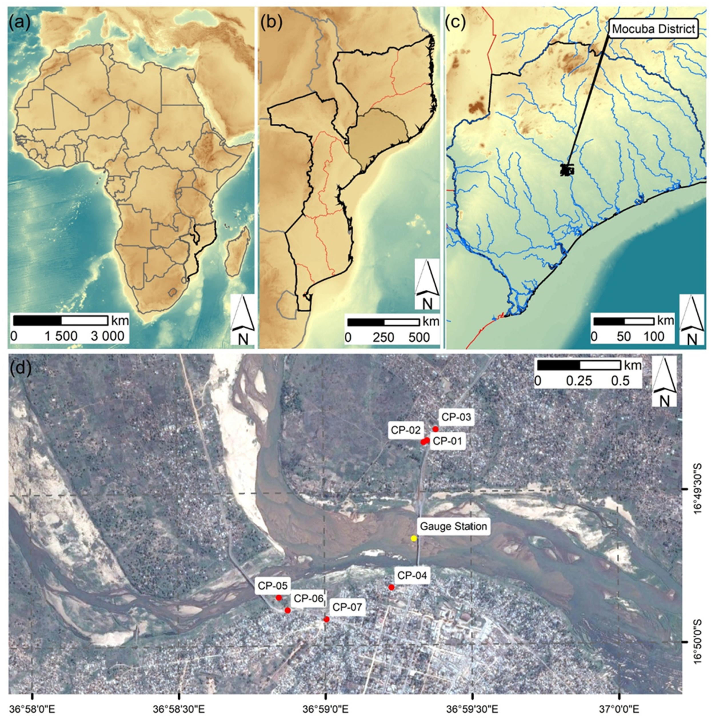
The city of Mocuba is located in the Zambezia region of Mozambique, about 100 km inland from the capital of Zambezia Province, the port city of Quelimane. The city of Mocuba has a population of about 70,000 people, but this rises to 230,000 people for the whole district of Mocuba. The city of Mocuba is located on the banks of the Licungo River (
Figure 1), just downstream from the confluence of this river with its tributary, the Lugela River. Most of the urban area of Mocuba is located on the right bank of the Licungo River, where a somewhat chaotic urban development can be observed, composed of old buildings from the colonial era (Mozambique was a Portuguese colony until 1975), and other, more modern buildings of poor construction quality. These low-quality, generally single-story buildings are the most common approaching the banks of the Licungo River. For this reason, the vulnerability of the buildings is considerable. Available information [
49] for the Mozambique country in general indicates estimated damages of about 75–80 EUR m
−2 in rural areas and about 400 EUR m
−2 in urban areas, when a 2-meter flow depth affects buildings. It is clear that these average figures cover very different situations. The same data indicate that for a 2-meter flow depth, the damage factor for buildings (building plus contents) is close to 85%.
On the other hand, the Licungo River extends over an area of approximately 30,000 km2, entirely within the territory of Mozambique. The headwaters of the river, north of the city of Gurue, are located in the mountainous reliefs whose summit is located in the Namuli Peak (with an altitude of 2419 m a.s.l), where intense rainfall feeds the flooding process at the mid and lower Licungo River basin. In fact, the location of Mocuba city could be used as the upper limit of flood-prone areas of the Licungo River basin. These intense rainfall events are frequently linked to the activity of cyclone systems in the Pacific Ocean.
These heavy rainfall events have produced at least 10 flooding events in the Mocuba District since the middle of the 20th century, according to information available in the International Disasters Database [
1]. Most catastrophic events are dated 1970, 2001, 2013, 2015, and 2019; in the two more recent events, the intense rainfall had its origin in the coalescence of two Pacific cyclones at the same time (the Chezda and Bansi cyclones in 2015, and the Idai and Kenneth cyclones in 2019).
2.2. The January 2015 Heavy Rainfall and Flooding Event
According to the Dutch Risk Reduction Team Report [
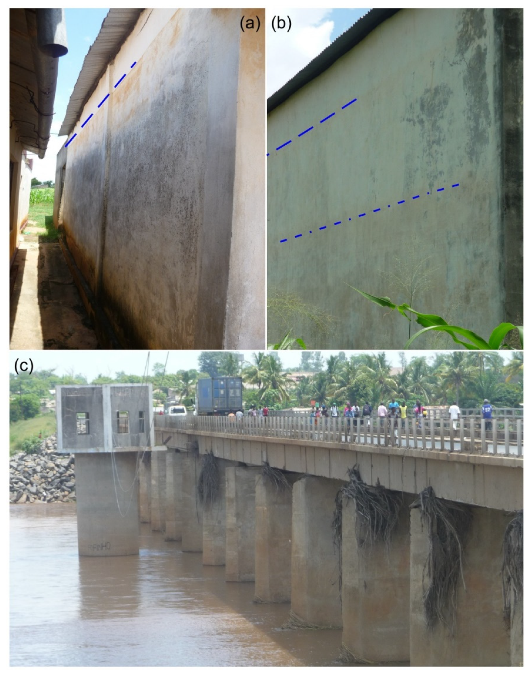
50], the 2015 flooding event lasted for approximately one month in the Licungo lower basin, beginning on 11 January 2015 and reaching its peak on 12, when the waters reached a depth of more than 12 m at the Mocuba gauging station and one of the bridges over the Licungo River collapsed. In Mocuba, the water levels dropped from 13 to 16 January 2015.
The flooding event was fed by an intense rainfall (with up to 590 mm [
51] over the month of January recorded in Mocuba, although other sources [
50] put the figure as high as 700 mm), which was related to a 30-year return period [
51], and rainfall intensity on 11 January 2015 was above 60 mm h
−1 [
50] according to Meteosat data. Considering that all the rainfall over the Licungo River basin contributed to the river discharge in Mocuba, the maximum peak flow estimations range from 13,000 to 19,000 m
3 s
−1; much higher than the estimation of the Directorate National of Water from the gauge station rating curve (about 6500 m
3 s
−1) [
51].
As a consequence of this extreme natural event, the damage for the whole area affected in the provinces of Zambezia and Nampula (Mozambique) was around USD 371 million (2.4% of the national GDP) [
51]., while the tasks of early recovery, post-disaster recovery, and vulnerability reduction were estimated at a total amount of USD 490 million. The post-event operations of emergency and recovery carried out by the International Federation of Red Cross and Red Crescent Societies helped 1588 households and 7940 people [
52] in the Mocuba District. According [
51] to the National Institute for the Management of Natural Disasters of Mozambique, registered casualties amounted to a total of 155, 10 of which took place in the city of Mocuba.
2.3. Hydro-Meteorological Data
Peak flow data were available for Mocuba city due to the presence of a gauge station with a non-continuous record from 1943 to 2014. The record of annual maximum peak flow derived from gauge station data is 69 years long, although personal communication from Mozambican technicians highlights a limited trust in higher peak flow values, due to deficiencies in gauging station measurements at times when flows rates are very high.
Assuming these measurement limitations, three extreme distribution values (Gumbel, generalized extreme values (GEV), and two-component extreme values (TCEV)) were fitted by the maximum likelihood (ML) method to obtain the relationship between peak flow rate and T-year return periods (
Table 1). Further, two-flow frequency analyses (FFA) were carried out considering the January 2015 peak flow (of which the value was estimated by field data [
51]) as non-systematic data, first as exact censored data (18,000 m
3 s
−1), and second as censored data (range or double limit data—13,000 to 18,000 m
3 s
−1).
The field data campaign after the January 2015 flooding event, accompanied by Mozambican technicians from the “Universidade Pedagógica de Mozambique”, in Mocuba city, allowed us to obtain the topographic data of seven control points linked to buildings affected or not affected by the flooding event. In the case of affected buildings, flow depth height data were collected.
2.4. Surface Terrain Data—Global DEMs
Several free global DEMs have been used to carry out a comparison regarding the performance of hydrodynamic simulations for flood-prone area delimitations and hazard analyses in sparse-data regions. An overview of selected free global DEMs, and their main features are given in
Table 2. In summary, their original spatial resolution is between 30 and 90 m, and they have been generated either from optical sensors (as is the case of ALOS and ASTER DEM) or by InSAR techniques (as is the case of SRTM, TanDEM-X, or Copernicus DEM).
Two of these are the main sources of data of the currently most used free global DEMs: First the SRTM, from which other DEMs are derived, such as the Bare Earth DEM (BEST DEM, O’Loughlin et al. [
55]), which involves removing the vegetation artefacts present in the original SRTM DEM; the MERIT DEM, in which errors are reduced by removing absolute bias, stripe noise, speckle noise, and vegetation bias (Yamazaki et al. [
33]); or the NASA DEM (Buckley et al. [
57]), which has been developed by completely reprocessing the SRTM radar data and then merging it with refined ASTER GDEM elevations. The second main data source is the TanDEM-X [
59], from which the recent Copernicus DEM [
58] derives, by terrain (spikes, voids, noise, and negative elevation) and hydrological (oceans, lakes, rivers, islands, or bridges) editing.
The group of free global DEMs used for hydrodynamic modelling in the city of Mocuba is used in the format in which they can be downloaded from their respective file servers (
Appendix A). The only processing of the data, with the aim of obtaining a homogeneous 3D mesh in the Iber software, consisted in resampling the data to a similar spatial resolution. The ESRI ArcGIS 10.6 environment was used for the process of resampling, and a value of 10 m was selected as the common spatial resolution of all DEMs.
Most of the DEMs used can be considered digital surface models (DSM), in which vegetation, buildings, water bodies, etc. are included. These DSM characteristics mean that they should only be used with caution in flood models [
19]. As pointed out by Archer et al. [
37], the processing and filtering of original data can produce an improvement in free global DEMs. However, for this assessment the DEMs have been used without any processing or filtering (except for those where the original downloaded data were already subjected to these treatments). This was done in this way with the idea of trying to replicate the analyses that could be carried out by public authorities responsible for flood risk management in developing countries, as these are likely to be the most frequent users of this type of DEM. In more economically developed countries, the analysis is likely to be carried out using higher spatial resolution topographic information, mainly LiDAR data. Therefore, we understand that end users in these developing countries will not carry out the complex tasks of processing and filtering the original topographic information, but will use the data as obtained from the web servers.
2.5. Mocuba City Urban Data
The urban Mocuba city building footprint at vector format was obtained from the OpenStreetMap [
60] dataset. The OpenStreetMap (OSM) is a geographic database with a worldwide coverage, which is constantly growing and ensures regular updates in terms of the accuracy and completeness of the data, so nowadays it is considered reliable [
61,
62]. The OSM has been previously used for flood vulnerability analysis [
63] with good results, since it does not solve all the problems linked to the vulnerability of buildings due to their shape and constitution, but data are consistent and openly accessible, which makes it easier and more cost effective to transfer vulnerability models to other regions. Although the OSM database does not include data about inhabitants per building, it can be a good approach (and probably the best public available data for Mocuba city), both regarding the number of buildings in the flood-prone area and the number of buildings within different building stability hazard areas.
2.6. Methodological Approach
The methodological approach of the present assessment could be divided into three main groups. The first group includes the use of available hydro-meteorological data (annual peak flow series) for FFA, with the aim of defining the peak flow value related to different return periods. The results of this FFA allow us to determine the frequency of different peak flow magnitudes.
Those peak flows for the T-year return period were used for hydrodynamic modelling with the free global DEMs (the second main group of working tasks) under consideration, so lower and higher peak flows allow one to compare the shape and extension of flood-prone areas. For a peak flow value, the hydrodynamic models are similar except for the topographic data, so the differences in results can be related to this variable rather than the combined effect of a group of variables.
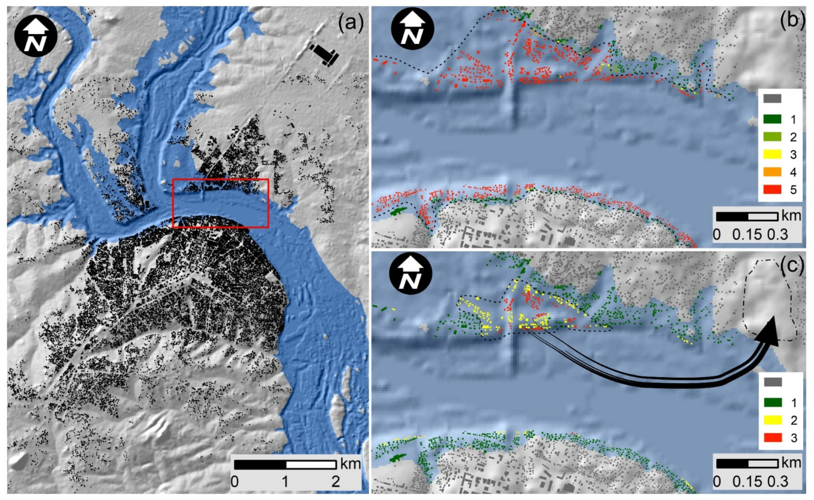
Finally, the third main group of working tasks includes those analysis for a calibration of the results obtained with the different hydrodynamic models, based on their comparison with the available field data (
Figure 2), as well as with the rating curve of the gauging station located in the city of Mocuba. Furthermore, we selected the best option between the different hydrodynamic models for flood hazard assessment by defining the areas and number of buildings where the hazard level of human loss of stability due to flooding characteristics is high, according to the model of Russo et al. [
64].
3. Results
3.1. Flood Frequency Analysis of the Annual Maximum Peak Flow Value Record
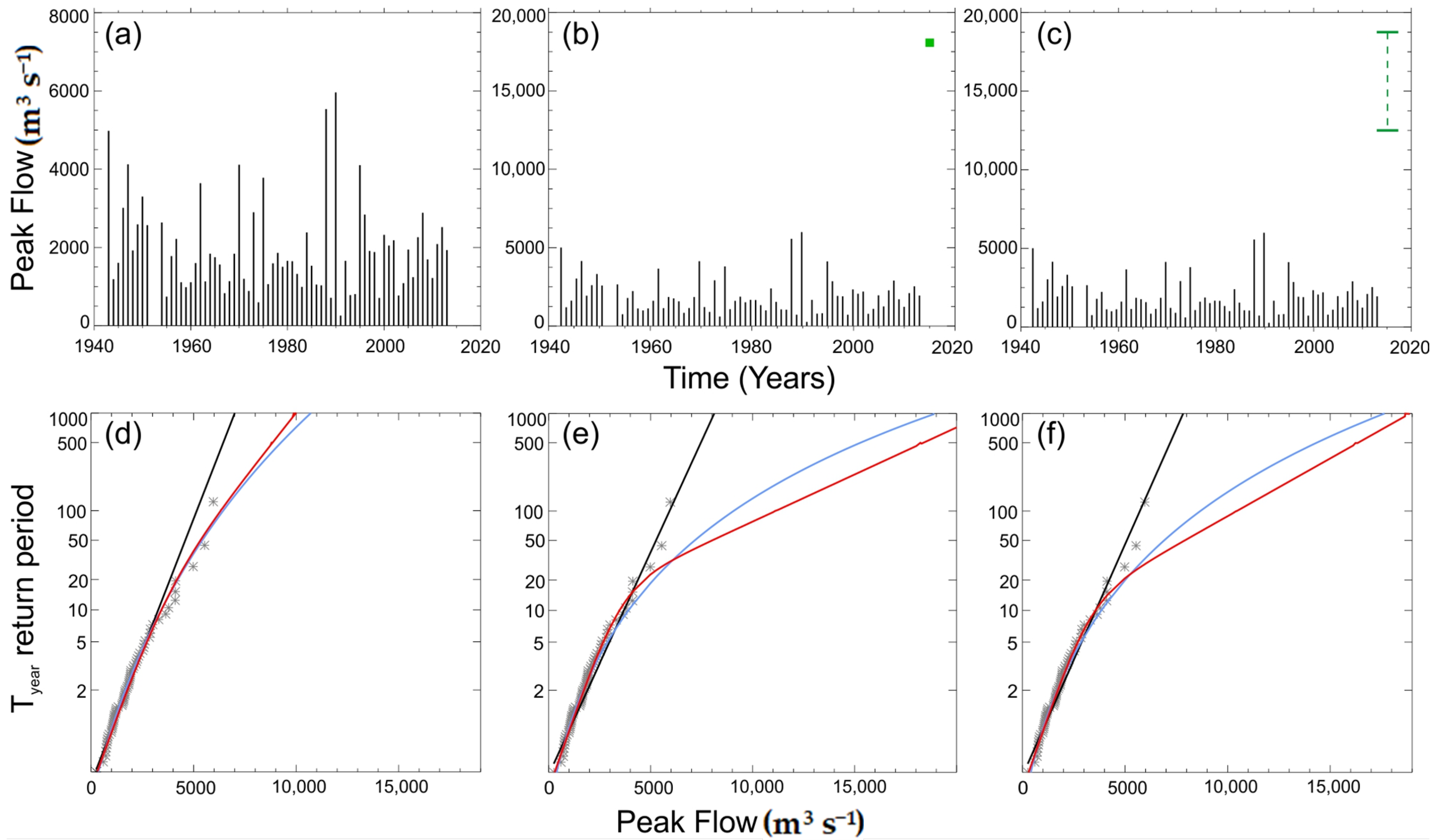
The results of the FFA (
Table 1) show significant differences when using only systematic data or systematic and non-systematic data; especially for high return periods (
Figure 3) and GEV and TCEV distributions. These results highlight the importance of working with representative data records, which include events of high magnitude. Thus, the absence of these high magnitude events (collected as systematic or non-systematic data) causes an underestimation of the magnitude of the process (in this case, a river flood) with respect to its relative frequency of occurrence.
From the first FFA (only systematic data), a 500-year return period peak flow value of 6451 m
3 s
−1 is obtained using Gumbel distribution, which is closed to the peak flow reported by the Mozambique Directorate National of Water [
51]. However, from the rating curve of the gauge station, the 500-year return period peak flow could be associated with a 9.5-meter flow depth value, far from the 12 m of flow depth obtained from field data for the January 2015 flood event [
51]. When using GEV or TCEV distributions, the peak flow value for the 500-year return period is increased up to values of 9277 and 8830 m
3 s
−1. Those peak flow values can be related to flow depth values of about 10.75 and 10.6 m, which are still lower than the field data value for the January 2015 flood event. Furthermore, although the January 2015 flooding event is regarded as probably the most catastrophic event in the recent history of Mozambique, other catastrophic events were dated in 1970, 2001, 2013, and 2019, so the frequency of catastrophic events is not too lower than a 200- or 500-year return period. Higher peak flow estimations [
51] shall be related to a T-year return period of up to 10,000 years or more, which may be considered an unrealistic estimate.
When non-systematic data are taken into consideration in the FFA, peak flow values for low-frequency events are significantly increased. This effect is mainly observed for FFAs carried out using the GEV or TCEV distribution functions, as these functions have a higher curvature capacity to adapt to sharper increases of the peak flow value with respect to its frequency. Thus, the peak flow value estimated by the Mozambique National Directorate of Water may be associated with a T-year return period lower than 50 years (a return period of about 35 years). Against this, a peak flow estimation ranging from 13,000 to 18,000 m
3 s
−1 [
52] is related to a T-year return period higher than 10,000 years using the Gumbel distribution, while, when GEV or TCEV distributions are used, that peak flow is related to a 500- or 1000-year return period. This difference points towards the effect of the use of different distribution functions, and the necessary knowledge of rainfall or flow characteristics at the study site.
From
Figure 3, we can observe that Gumbel distribution probably underestimates peak flow values for higher return periods, while GEV and TCEV distribution show more similar values. The underestimation associated to the Gumbel distribution function has been highlighted previously [
65,
66], and it is not a new feature of this study. It can also be noted that the use of estimated field peak flow for the January 2015 event as non-systematic data provide different results depending on how these data are considered. When the January 2015 data are used as exact values, the peak flow values linked to higher return periods are greater than those values when the January 2015 peak flow is used as a range value. In this case, and due to the uncertainty in the field estimation of the January 2015 peak flow, the use of this value as a range could be the more realistic option.
3.2. Free Global DEMs and Hydrodynamic Modelling
The comparison of results from all free global DEMs used is going to be made for three different flow rates: one related to high-frequency flow rates (10-year return period); another related to medium-to-low-frequency flow rates (about 100-year to 500-year return periods, depending on the distribution function considered); and finally an extreme event such as the January 2015 flood, with an estimated peak flow of 18,000 m
3 s
−1 [
51].
For each of these three sets of results, the shape of the flood-prone area, its spatial continuity and the range of values, as well as the values of the slope of the water surface and its spatial distribution were analyzed. The latter analysis was carried out with the aim of determining the presence of peaks and sinks in the DEMs, and on the assumption that the water surface should have a low slope (approximately similar to the slope of the channel) with a reduced spatial variability.
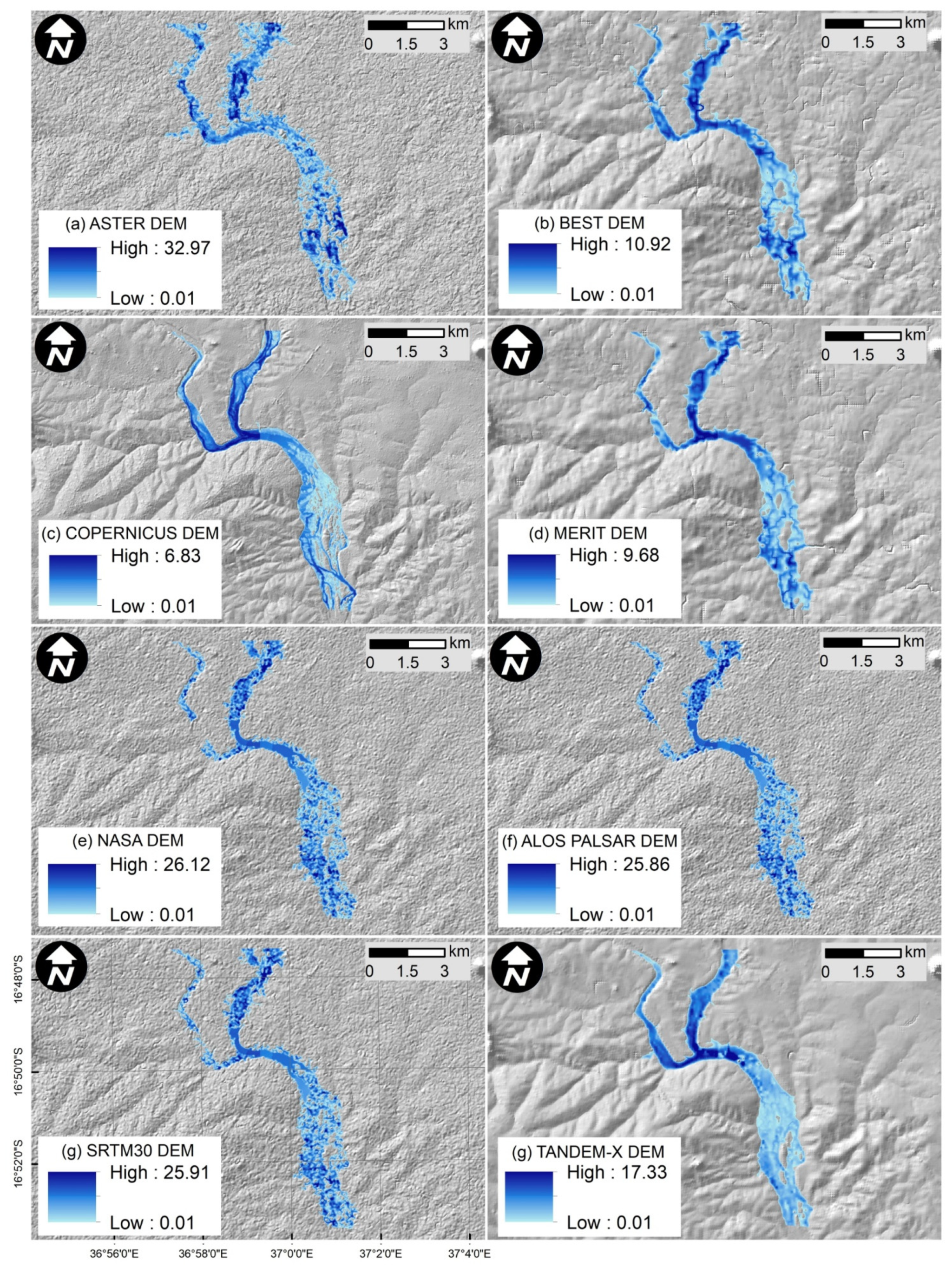
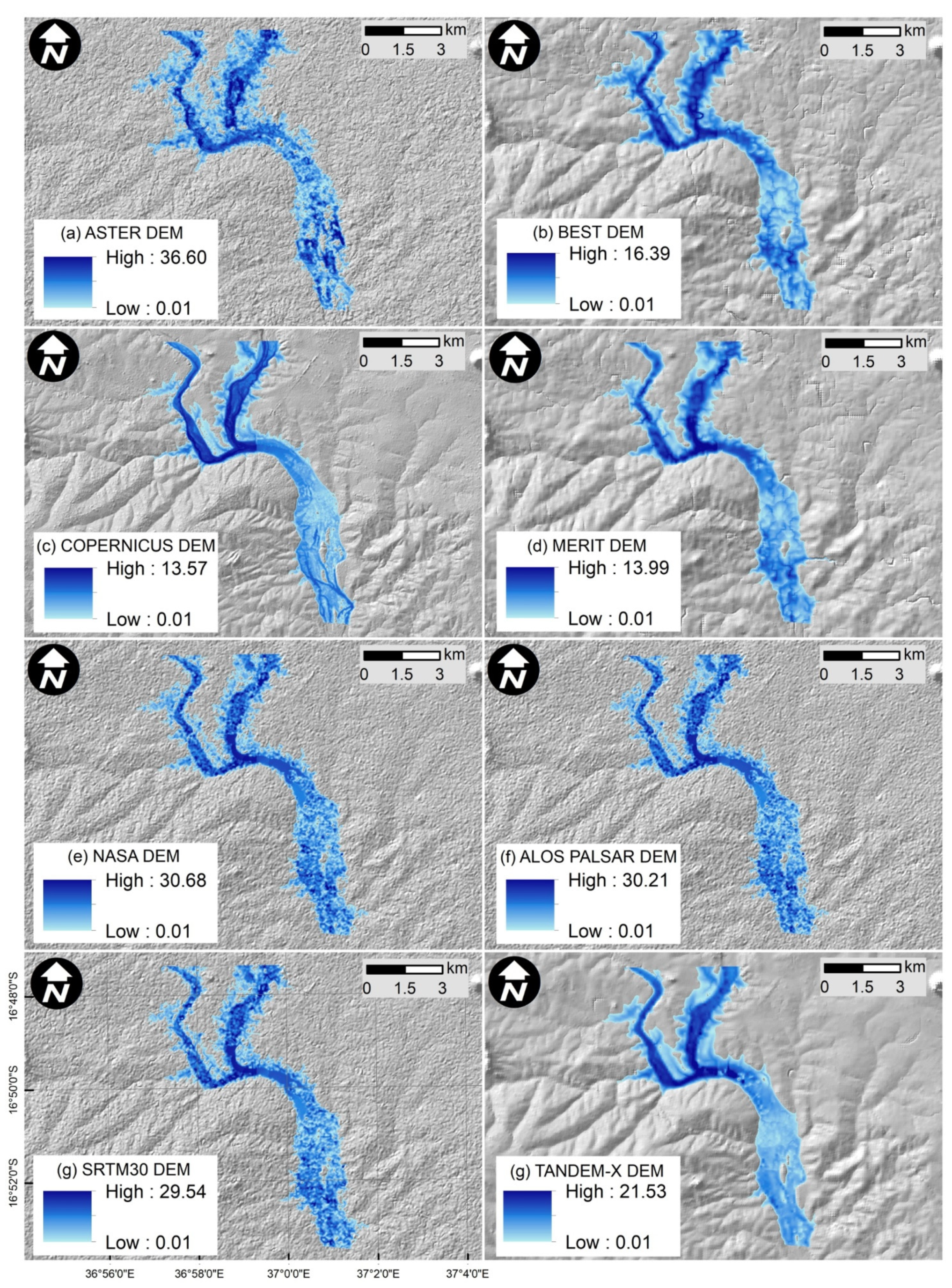
For the results related to the 10-year return period peak flow (
Figure 4), two main groups of results can be established on the basis of their visual appearance and spatial continuity. The first group may include the ASTER, NASADEM, ALOS Palsar, and SRTM30, which show high variability in flow depth values for neighboring or adjacent pixels, a lower spatial continuity, and all of them show an artificial appearance surface in the vicinity of Mocuba city. On the other hand, the BEST, Copernicus, MERIT, and TANDEM-X models show a lower variability in flow depth values for neighboring or adjacent pixels, and a higher spatial continuity. From the second group, the BEST and MERIT models show some artificial features like little channels in the flooding area, which change their flow direction at 90-degree angles, possibly conditioned by the height distribution in the pixels.
The previously defined DEM groups are supported by maximum flow depth values too. Thus, the group including ASTER, NASADEM, ALOS Palsar, and SRTM30 DEMs shows flow depth values of up to 30 m or more (36.5 m for the ASTER DEM), while the second group (the BEST, Copernicus, MERIT, and TANDEM-X models) shows flow depth values ranging from the 13.5 m of Copernicus DEM to 21.5 m for the TanDEM-X. The previous maximum values are related to the January 2015 peak flow, just when the flow depth differences between two groups are at their lowest. This effect could be explained by the fact that the maximum values of flow depth in the first group are associated with the presence of artificial depressions within the DEMs, which are the origin of the presence of such high values of flow depth.
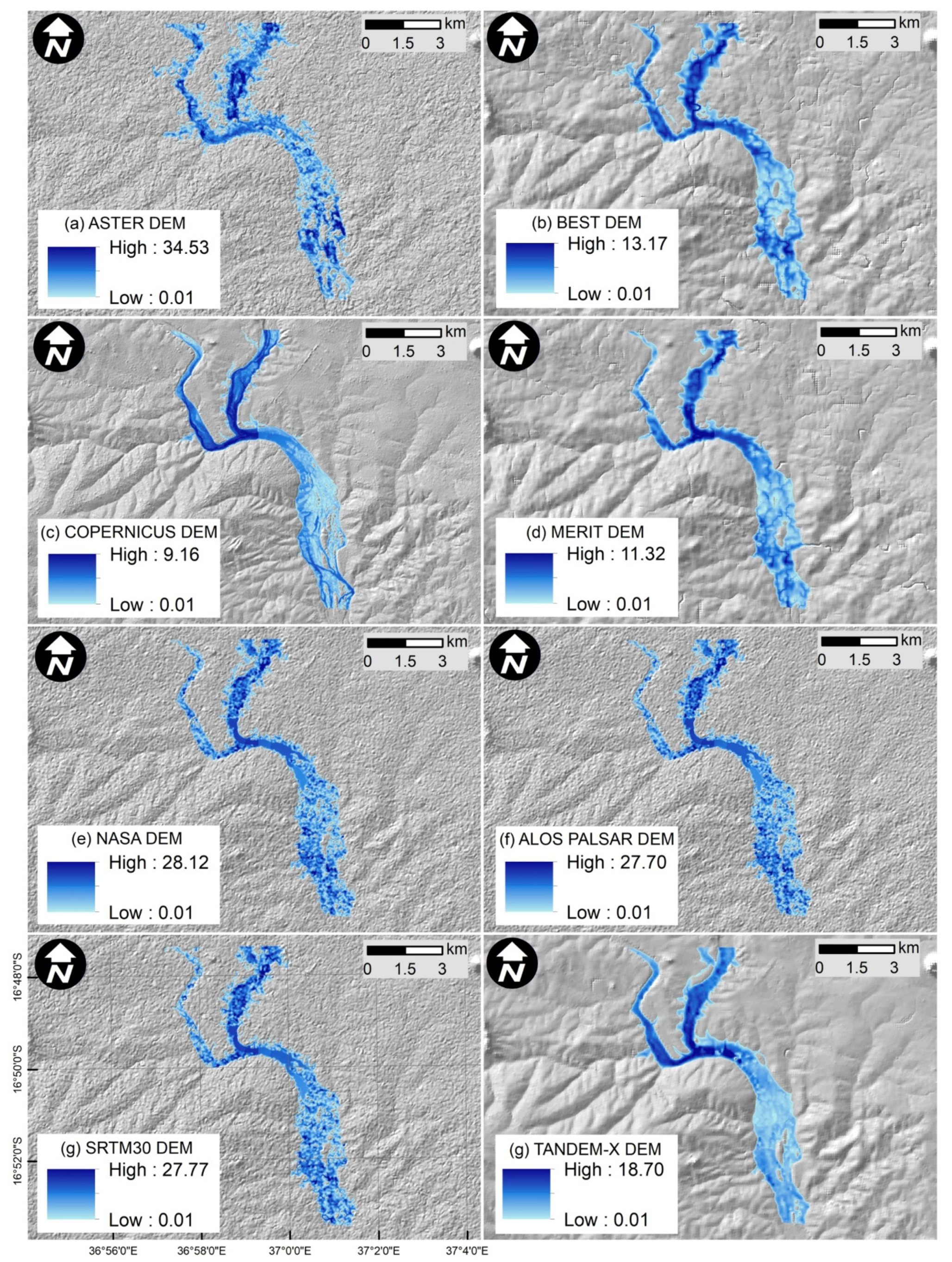
When considering the results related to the 100- to 500-year return periods (
Figure 5), the description of results is very similar to the previous one. The same two main groups can be established, and the same models are included in each group. Of course, the flood-prone areas are larger than those related to the 10-year return period and the spatial continuity is also greater for all models. When observing the results of the January 2015 peak flow models, the same conclusions are observed, so the BEST, Copernicus, MERIT, and TANDEM-X models show the better performance. From all models, the Copernicus DEM probably shows the most realistic results (
Figure 6), where flow depth variations in the channel appear to be related to the presence of sand bars, rocky outcrops, and inner channels. Although BEST, MERIT, and TanDEM-X models show a good performance too, the flow depth variations observed in the results are not too easily related to inside channel forms and deposits.
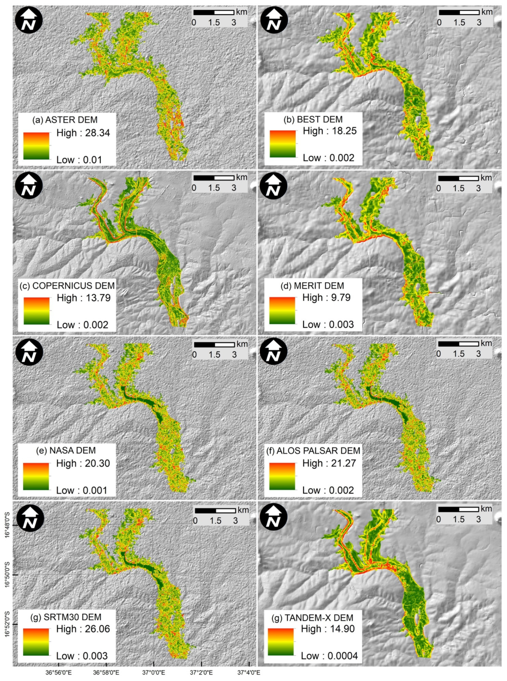
The results of water surface slope maps look quite similar to those of the flow depth, but some differences can be pointed out. On the one hand, the high variability in the spatial distribution of slope values can be observed too for the first group of DEMs (ASTER, NASADEM, ALOS Palsar, and SRTM30 DEMs), and they do not show a clear spatial pattern, and the slope variability is clearly lower for the second group of DEMs. This trend of high spatial variability cannot be interpreted as a succession of riffles and pools in the river channel, but rather resembles a network of pools as previously noted [
6] in the case of the SRTM model.
In the other hand, all DEMs derived from SRTM data (SRTM30, BEST, MERIT, and NASADEM; the ALOS Palsar DEM) show a homogeneous and low slope area just in front of Mocuba city (
Figure 7), which corresponds to a flat surface observed in DEMs (which may be due to radar shadows). This “non-natural” feature in water surface slope maps is partially blurred in BEST and MERIT DEMs, those in which filters were applied by developers to remove vegetation and noise.
3.3. Comparison of Hydrodynamic Model Results and Field Data
The comparison of hydrodynamic model results against field data was driven in two ways. First, the flow depth values of each hydrodynamic model (including all DEMs and T-year return periods) were plotted against the Mocuba gauge station rating curve with the aim to highlight deviations from the rating curve and select the best option of free global DEM. The second time, the flow depth results from each combination of “DEM–T-year return period” were compared to the flow depth values of the seven control points collected in the field work after the flooding event. Those seven control points include three water heights measured from building watermarks, and four non-flooding points on both sides of the Licungo River, so they allow one to define the spatial extension of flooding at the January 2015 event.
The two analyses were carried out using the mean absolute error (MAE) and the Nash-Sutcliffe efficiency (NSE) statistical indexes, as shown in Equations (1) and (2).
where
is the flow depth of the ith cell for the “modelled scenario”,
is the flow depth of the ith cell for the “observed scenario”, and
is the number of cells used for the analysis.
where
is the flow depth value of the modelled scenario,
is the flow depth value in the observed scenario, and
is the mean flow depth value for the observed scenario.
The results obtained for the gauge station and control points are shown in
Table 3. In both cases, the results linked to Copernicus DEM are the best option and they show the closest values to the Mocuba gauge station rating curve and the palaeostage indicator (PSIs) marks. For the first analysis, which plots flow depth values (from all free global DEMs) against the gauge station rating curve, the ASTER and TanDEM-X DEMs show the worst results and the other DEMs show MAE values ranging from 0.21 (Copernicus DEM) to 0.38. A similar trend is observed for NSE index, with the best result (0.75) linked to the Copernicus DEM. These results highlight the Copernicus DEM as the best model to reproduce the behavior of the waters (flow depth) within the Licungo riverbed. The error of 0.21 m shown by the MAE index is quite homogeneous regardless of the return period considered and shows an efficiency of 75% (NSE value) in reproducing the behavior of the rating curve of the gauging station.
The second analysis plots flow depth values against several control points, which include both 2015 flooding and unflooded areas. The results linked to ASTER DEM are the worst once again, but TanDEM-X DEM is now the second best option after the Copernicus DEM and very similar in results to the MERIT DEM. The Copernicus DEM is the only one in which the flow depth values in all the selected non-flooding control points were equal to 0.00 m. The MAE index for the Copernicus DEM shows a mean deviation of 0.44 m from field data and an efficiency of 81% (NSE index) reproducing real flow depth values. As the flow depth values in the non-flooding areas are reproduced exactly by the Copernicus DEM model, it is clear that the error at the control points in the flooded areas is higher. This could indicate that the peak flow value associated with the January 2015 event could be even higher than previously estimated.
None of the other models show a uniform trend in the relationship between modelled and real flow depth values. Thus, in the rest of the models, we can observe control points in which the modelled flow depth value is greater than the one observed, while in other control points the relationship is inverse. Thus, this heterogeneity in the results cannot be related to the peak flow value, but to possible errors in DEMs and their deficient topographic surface representativeness.
The MERIT and TanDEM-X models offer the best results after the Copernicus model. The results for both models are similar, and slightly better in the MERIT model. This is in agreement with previous reports by Archer et al. [
37], who already indicated that the TanDEM-X model (in its non-free access model, with a higher spatial resolution of 12 m), without additional surface artefact processing, improved on the performance of the SRTM model but not on the MERIT model in flood estimation.
3.4. Flood Hazard Assessment in Mocuba City
The hydraulic model developed upon the Copernicus DEM, which showed the best results in the previous section, was used to define the dragging people hazard zone according to the Russo et al. [
64] model. The flood hazard model uses the flow depth and flow velocity variables to define up to five different hazard levels (from low hazard for adults and children—value 1, to extreme hazard for adults—value 5). In the absence of building scale census data (including inhabitants per building), the analysis was carried out at building scale by using data from the OpenStreetMap database [
60].
The results (
Figure 8a) from hydraulic modelling show that a total of 2113 buildings in Mocuba city were affected during the January 2015 flooding event (using an estimated peak flow of 18,000 m
3 s
−1). This value is greater than the number of households (1588) helped by the International Federation of Red Cross and Red Crescent Societies [
52] in the Mocuba District, but it is very close to the number of buildings (1452) where flood hazards are moderate to extreme. From the flood hazard analysis, attention must be paid to the high number of buildings (
Figure 8b) where the hazard level is extreme (1422), which highlights the magnitude of the January 2015 flooding event and its associated high flood risk.
Other damage models are focused on building stability or damage rate in relation to both flow depth and velocity variables. The Pistrika and Jonkman model [
67], where the “dv” variable represents the product of flow depth by flow velocity, considers three damage levels and it was used in Mocuba city.
dv < 3 m2 s−1 yields only ‘‘inundation damage’’;
3 m2 s−1 ≤ dv < 7 m2 s−1 1 yields ‘‘partial damage’’;
dv ≥ 7 m2 s−1 yields ‘‘total destruction’’.
The results from the Pistrika-Jonkman model show that the majority of buildings are affected by “flood damage” hazard level (1814 buildings of the 2113 affected by the January 2015 flooding event). Only 82 buildings show a “total destruction” damage level (
Figure 8c), but these data cannot be compared to other data sources, such as the International Federation of Red Cross and Red Crescent Societies [
52] report. Neither the report [
52] nor the field data point to the occurrence of buildings collapsing, due to the absence of any commentary in the report or by the inhabitants.
4. Discussion
The FFA results show the uncertainty associated to the distribution function used and the consideration in the analysis of only systematic or systematic + non-systematic data. Anyway, this is not one of the main objectives of the present assessment, but it shows the clear dependence of an accurate estimation of higher return periods on the presence of extreme events in the systematic records, or the use of non-systematic data (e.g., [
68,
69,
70]). Thus, it is highly probable that the real return period for the January 2015 flooding event is lower than 500 years, because other known catastrophic events (1970, 2001, 2013, and 2019) may be underestimated in the peak flow record derived from the gauging station located in the city of Mocuba. The maximum peak flow for these other catastrophic events (except the 2019 event, which lies out of the temporal range of available time series) is only 4114 m
3 s
−1 in 1970, which is too far from the 13,000 to 18,000 m
3 s
−1 [
51] estimate for the January 2015 event. Therefore, if we take into account that the extreme peak flow values may be underestimated (something that some Mozambican technicians already pointed out in personal communications), the frequency or return period associated with these extreme events must be significantly lower than that obtained in this FFA.
As regards hydraulic modelling, the results show the effect of DEM artefacts due to errors in topographic data. All these artefacts in the river channel could be partially removed by hydrological correction processes, which improve their suitability for simulating floods [
32,
37,
71] when compared with original DEMs due to the correct representation of the rivers and associated channels. However, no hydrological corrections have been carried out (beyond those previously carried out, and which are integrated in the data that can be downloaded from the web servers where each model is available) to maintain equal conditions for all DEM models, as neither Copernicus nor TanDEM-X show a clear need for hydrological corrections. On the contrary, in the case of the Copernicus model, the width of the Licungo River as it passes through the city of Mocuba allows for an efficient reproduction of the channel cross-section shape with the original spatial resolution of the DEM. This is another important factor to take into account in hydraulic modelling, which works with low spatial resolution DEMs, as previously pointed out by Sanders [
6]. In fact, this may be a key point for future works involving Copernicus DEM, analyzing its ability to correctly reproduce the cross-section of narrower channels, and thus being able to produce useful results for flood hazard management in such scenarios.
With the aim to check the quality of the result of the hydraulic models, flow depth values were compared both with the Mocuba gauge station and with several field control points. Comparing the modelled flow depth values against the Mocuba gauge station rating curve involves uncertainty due to the characteristics of the gauge station itself. Probably, the most important factor is the Licungo riverbed mobility due to fluvial incision and deposition processes, which can produce variations over time in the flow depth–flow rate relationship for the gauging station [
72]. The cross-sectional shape and elevation are critical parameters for a correct flow rate estimation, as well as in the determination of paleo-flow rates [
73], and both parameters change over time due to erosional and depositional process associated to river dynamics. Thus, increases and decreases in flow velocity imply changes in the sediment transport capacity of water, which is directly related to the processes of fluvial erosion (linked to areas of higher flow velocity) and fluvial sedimentation (linked to areas of lower flow velocity, or when there is a decrease in flow velocity). All these variations occur during a river flood event and, as a consequence, cause variations in the shape of the channel cross-section, which are responsible (by modifying the drainage capacity of the channel) for altering the flow depth-flow rate relationship for that section of a river. Those changes are observed in the Mocuba gauge station record, so the rating curve was calculated by using only the more recent records (2000 to 2014), trying to avoid errors caused by older cross-sectional channel shapes that would have other associated flow depth-flow rate relationships. Using the more recent flow depth-flow rate data can limit the uncertainty linked to fluvial incision and deposition processes, but it can limit the availability of extreme event data; thus, a certain degree of uncertainty still remains.
Calibrating the results from flood models with water level data is usual for one-dimensional (1D) simulation models [
3,
74,
75,
76], while 2D simulation models tend to be calibrated and validated by comparing extensional flooding areas [
77,
78]. In the present assessment, a 2D simulating model (Iber) was used for hydraulic modelling, but a calibrating of the model through flooding extension is not available due to the lack of observed (field) data or remote sensing data on the event date. Thus, we calibrated the performance of the models against a set of water level measurements [
9,
15] in the study area.
Another way of calibrating hydraulic models is through the use of “
citizen science”, a calibration method that has been increasingly used since the 2010 decade. “
citizen science” involves different types of data acquisition and a review of the “
state of the art” could be found in Assumpção et al. [
79]. Although most such cases are located in developed countries (e.g., [
80,
81]), some positive assessments have been carried out in developing countries too (e.g., [
82,
83]); as highlighted by the experience of Sy et al. [
82], the use of “
citizen science” could help reconstruct past flood events and open up an available path for obtaining useful flood data in areas of scarce or unavailable flow data records.
When flood hazard analysis was carried out in Mocuba city, the results from the two hazard models used [
64,
67] gave results that are in agreement with the field assistance works carried out by the International Federation of Red Cross and Red Crescent Societies [
52]. However, some differences can by observed in the number of damaged buildings and damage levels. Building materials (masonry, bricks, woods, etc.) or types (elevated floor level, with or without a basement) cause significant changes in the damage rate associated with flow depth values, as can be seen in the compilation of Shrestha et al. [
84]. Thus, the quantitative results of the damage model should be viewed with caution, and it is likely that they should be used through a more qualitative approach.
Finally, the results obtained for Mocuba city could be of help to local natural hazard managers, the Zambezia regional government, or the Mozambican government with land planning and flood risk management and mitigation. Thus, the number, location, and spatial distribution of buildings at high flood hazard (
Figure 8c) could help design plans for the relocation of the population at risk of flooding to other, less hazardous areas of the city.
5. Conclusions
The city of Mocuba (Mozambique) has been selected to perform an assessment of free global DEMs and hydrodynamic modelling for flood hazard analysis. The choice of Mocuba city was due upon two main criteria: the city belongs to a developing country (where the availability of high-resolution DEMs is practically nil) and there is a repeated occurrence of flood events (the one that occurred during the month of January 2015 being that with the highest recorded magnitude).
The visual and statistical analysis of results from hydrodynamic models (for each of the eight DEMs) highlights the improved performance of the Copernicus DEM, the most recent of all DEMs used. Thus, a visual analysis of flow depth parameters shows more natural trends in its spatial variability, which could be related to the presence of riff and pools in the riverbed. This trend of results is less evident for TanDEM-X and MERIT DEMs, and it is totally unrecognizable for the rest of the models, where the variations in flow depth cannot be due to the natural forms of the channel but to the presence of topographic errors.
The statistical analysis of results through the use of MAE and NSE indexes point to the same conclusions. The performance of the Copernicus DEM is an improvement over all the other ones, and this free global DEM is the only one where the flow depth value in all the selected non-flooding control points was equal to 0.00 m. The results shown by the Copernicus DEM against field data (Mocuba gauge station and field control points) are much better than with any other free global DEMs.
The hydraulic model (using the Copernicus DEM) outputs, such as flow depth and flow velocity, have made it possible to define different flood hazard areas in Mocuba city. The use of the dragging people flood hazard model as well as building structural stability models have shown results (number of buildings at high hazard levels) that are in agreement with previous reports, such as that of the International Federation of Red Cross and Red Crescent Societies.
There are multiple previous research papers that advocate the need to improve the quality of the free global DEMs in order to develop more reliable flood hazard maps. Most of these previous studies do not use the last version of the Copernicus DEM, because it was launched barely more than a year ago. However, in view of the results obtained in the present study, the use of the Copernicus DEM along with flooding evidence field data could be a reliable approach to flood hazard assessment in developing countries, or at least for those rivers whose dimensions (river width) allow for an acceptable reproduction of their shape with the spatial resolution of these free global DEMs. Anyway, the results obtained should not be interpreted as an amendment to two widely agreed upon proposals: the need to improve the spatial resolution and quality of the global models, and the need to promote citizen participation in the collection of field data to improve the calibration of hydraulic models for flood hazard analysis.


