Article

Micro-Climate Computed Machine and Deep Learning Models for Prediction of Surface Water Temperature Using Satellite Data in Mundan Water Reservoir

by
Sabastian Simbarashe Mukonza
1 and
Jie-Lun Chiang
2,*
1
Department of Civil Engineering, National Pingtung University of Science & Technology, No. 1, Shuefu Road, Neipu 91201, Pingtung, Taiwan
2
Department of Soil and Water Conservation, National Pingtung University of Science & Technology, No. 1, Shuefu Road, Neipu 91201, Pingtung, Taiwan
*
Author to whom correspondence should be addressed.
Water 2022, 14(18), 2935; https://doi.org/10.3390/w14182935
Submission received: 14 August 2022 / Revised: 5 September 2022 / Accepted: 15 September 2022 / Published: 19 September 2022

Abstract

:
Water temperature is an important indicator of water quality for surface water resources because it impacts solubility of dissolved gases in water, affects metabolic rates of aquatic inhabitants, such as fish and harmful algal blooms (HABs), and determines the fate of water resident biogeochemical nutrients. Furthermore, global warming is causing a widespread rise in temperature levels in water sources on a global scale, threatening clean drinking water supplies. Therefore, it is key to increase the frequency of spatio-monitoring for surface water temperature (SWT). However, there is a lack of comprehensive SWT monitoring datasets because current methods for monitoring SWT are costly, time consuming, and not standardized. The research objective of this study was to estimate SWT using data from the Landsat-8 (L8) and Sentinel-3 (S3) satellites. To do this, we used machine learning techniques, such as Support Vector Regression (SVR), Gaussian Process Regression (GPR), simple neural network (ANN), and deep learning techniques (Long Short Term Memory, LSTM, and Convolutional Long Short Term Memory, 1D ConvLSTM). Using deep and machine learning techniques to regress satellite data to estimate SWT presents a number of challenges, including prediction uncertainty, over- or under-estimation of measured values, and significant variation in the final estimated data. The performance of the L8 ConvLSTM model was superior to all other methods (R2 of 0.93 RMSE of 0.16 °C, and bias of 0.01 °C). The factors that had a significant effect on the model’s accuracy performance were identified and quantified using a two-factor analysis of variance (ANOVA) analysis. The results demonstrate that the main effects and interaction of the type of machine/deep learning (ML/DL) model and the type of satellite have statistically significant effects on the performances of the different models. The test statistics are as follows: (satellite type main effect p *** ≤ 0.05, Ftest = 15.4478), (type of ML/DL main effect p *** ≤ 0.05, Ftest = 17.4607) and (interaction, satellite type × type of ML/DL p ** ≤ 0.05, Ftest = 3.5325), respectively. The models were successfully deployed to enable satellite remote sensing monitoring of SWT for the reservoir, which will help to resolve the limitations of the conventional sampling and laboratory techniques.

1. Introduction

Water quality is a measure of a water body’s characteristics that include its thermal, physical, chemical, and biological properties [1]. SWT is a crucial water quality parameter indicator of the hydrological cycle energy balance, hence it has found useful applications in hydrology, meteorology, and climatology. Globally, the surface water temperature of aquatic ecosystems is rising, which is affecting aquatic ecosystems [2]. These climate-driven hydrological changes have resulted in increasing snowmelt [3], surface erosion caused by snowmelt/rainfall runoff, increasing suspended sediment concentrations [3], a decrease in dissolved gases, such as dissolved oxygen (DO) [3], proliferation of algal blooms [4], and ocean acidification [5]. Consequently, warming water bodies are resulting in a wide range of impacts, including loss of habitat for cold water fish species, low DO levels, and fish mortality, resulting from harmful algal blooms. Global water pollution is increasing and has a detrimental effect on the environment, human health, and economic development [6]. Despite rising global water pollution, there is a lack of monitoring data to determine the extent of the problem [7]. The traditional SWT monitoring techniques (such as infrared sensors and thermometers) are arduous, time-consuming, and rely on discrete sampling to provide only a small number of in situ data points at very low sampling frequency [8,9].
The use of satellites with high spatiotemporal resolution for monitoring water quality helps to reduce needless manual sampling, this also lowers sampling costs and time [8,9]. For optically active water quality parameters, such as Chlorophyll-a (Chl-a), Chromophoric Dissolved Organic Matter (CDOM), and Suspended Sediments (SS), retrieval models are established based on empirical, analytical, semi-empirical, and machine learning methods [10,11]. Chemical oxygen demand (COD), dissolved oxygen (DO), total nitrogen (TN), and total phosphates (TP) are examples of optically inactive substances that do not directly correlate with spectral characteristics, such as AOP/IOP/Radiative Transferee Equation (RTE). However, they can be measured as proxies for optically active parameters or by using artificial intelligence to establish the complex relationships that exist between them and various satellite sensor signals [10,11]. In contrast, SWT’s spectral features depend on thermal infrared and microwave activity, hence it is neither an optically active property of water nor can it be identified by proxies of optically active substances. Therefore, in order to approximate surface temperatures and surface salinity of water bodies, thermal infrared and microwave bands are helpful [11]. For instance, Sentinel-2 MSI is unable to monitor land surface temperature because it lacks thermal infrared bands; whereas Landsat-8 OLI/TIRS, which is equipped with a TIRS sensor, can measure thermal emissivity to estimate temperature [12]. Based on thermal infrared remote sensing, the split window method (SWA) and radiative transfer equation (RTE) are used to calculate the temperature pixel values in satellite images [12,13]. The output temperature calculated using satellite data is a discrete temperature value that represents a pixel of the water body’s surface under monitoring. This value is more likely to be influenced by micro-climate variables describing the thermodynamic and dynamic state of the atmosphere, i.e., atmospheric air temperature (AAT), relative humidity (RH), wind speed (WS), and precipitation (P). Several studies have focused on using satellite data to measure sea surface temperature (SST) [13,14,15,16,17], while only a very small number of studies have concentrated on inland waters [12]. Most of these studies have used sensors with high spatial resolution, such as MODIS [13,14,16], in order to monitor large coverage of SST. Similarly, Sentinel-3 land surface temperature (LST) products may be used to track the thermal characteristics of inland surface water because of their high temporal resolution despite having a coarse spatial resolution. Additionally, the improved spectral, radiometric, and spatial resolution of the Landsat-8 TIRS sensor makes it an ideal choice for monitoring inland surface water temperature [18,19].
The two satellites used in the study are Landsat-8 (launched on 11 February 2013) carrying the Optical Land Imager (OLI) and Thermal Infrared Sensor (TIRS) instruments, which offer images with a higher spatial resolution (30–100 m) but a low revisit time frequency of 16 days, and Sentinel-3A (launched on 16 February 2016) and 3B (launched on 25 April 2018). Sentinel-3 A/B is a twin constellation equipped with the Sea and Land Surface Temperature Radiometer (SLSTR) on board these satellites and has two thermal bands, at 10.8 and 12 µm, which acquires LST at a coarser spatial resolution of approximately 1-km at nadir [20]. In comparison to Landsat-8, the Sentinel-3 constellation has a shorter revisit time of less than two days, making it suitable for applications in near-real time analysis [20]. Furthermore, archived data for both sensors are made freely available by the Copernicus Open Access Hub via several platforms (https://scihub.copernicus.eu accessed on 31 July 2021) and the United States Geological Survey (USGS) via EarthExplorer or GloVis. Finally, the satellites’ planned life cycle for Sentinel-3 is expected to span 15 to 20 years [21].
Recent publications have shown the potential of satellites, such as Landsat-8, Sentinel-2, and Sentinel-3 data application for monitoring water’s optical properties [22]. Single sensors [22], multi-sensor data fusion [22,23], and inter-sensor performance comparison approaches have all been used by researchers in investigating water quality [22,23,24]. As an example, different optically active constituents in water affects the sensitivity of Landsat-8, Sentinel-2, and Sentinel-3 spectral bands in different ways. This investigation examined the claims of difficulties in retrieval of chromophoric dissolved organic matter (CDOM) absorption using Landsat-8 and Sentinel-2 band configurations [25]. However, a limited number of studies have investigated water’s thermal properties using satellites in inland water bodies [26]. These studies have been applying single sensors and only a limited number have used multi-sensor data fusion [26,27]. Therefore, this study seeks to investigate inter-sensor comparison between L8 and S3 multi-sensor data and design a two-factor ANOVA design to compare how satellite properties and different types of machine and deep learning methods affect the retrieval of SWT. In as far as our knowledge is concerned, there has not been prior work that implemented such an experimental design in this research niche to compare performances of different satellites. Furthermore, we propose that the various models being used should take into account how microclimate factors/variables affect SWT. Regression prediction was performed using machine and deep learning models based on input features, such as WS, RH, P, AAT, Landsat-8 derived SWT (SWTL8), Sentinel-3 derived SWT (SWTS3), and the response variable ground-truth SWT (SWTGT). To assess the ML/DL technique’s predictive power: GPR, SVR, ANN, LSTM, and 1D ConvLSTM were trained on the input and output dataset. Finally, we provide a method for producing satellite-SWT at a large spatial variation using ML/DL algorithms that takes into account a complex interaction of hydro-meteorological variables.

2. Materials and Methods

2.1. Study Area

Mundan Reservoir is located in Mundan Township, in Pingtung County, Southern Taiwan. It supplies water for domestic consumption in Pingtung County and irrigation use for the Hengchun area. Mundan Reservoir is situated downstream, upstream, and midstream of the Sihjhong River valley at coordinates (22°07′58″–22°09′07″ N and 120°46′40″–120°47′11″ E) (Figure 1). It is a floodpath lake with significant seasonal variations in water levels. It has three sampling points designated at geo-coordinates 22°8′1.6512″ N and 120° 46′52.6368″ E for point 1, 22°8′25.4508″ N and 120°46′57.2412″ E for point 2, and 22°8′49.578″ N and 120°46′56.3448″ E for point 3, respectively.

2.2. Data Collection and Image Preprocessing

This section, explains how in situ and satellite data were collected for specific use in this study. Furthermore, it provides the theoretical background including equations and software used during the data preprocessing stages. Based on the sampling conducted at points 1–3 (S1–S3), which are highlighted in the reservoir map in Figure 1, SWT ground-truth data for Mundan reservoir was obtained from the Environmental Protection Administration, ROC (Taiwan) database, hereinafter referred to as Taiwan EPA database. Temporal resolution of in situ measurements is 4 or 5 times per month and is dependent on the sampling plan as laid out by Taiwan EPA. The meteorological station COR341 on the map was used to measure and gather the micro-climate observational data variables. Satellite data from Landsat-8 (L8) and Sentinel-3 (S3) for the selected regions of interest and acquisition dates corresponds to Taiwan EPA sampling locations and time were collected from USGS (EarthExplorer (usgs.gov)) accessed on 31 July 2021 and Sentinel Hub (https://scihub.copernicus.eu/dhus/ accessed on 31 July 2021) databases respectively. The S3 and L8 images were processed using European Space Agency’s (ESA) SentiNel Application Platform version 8.0 (SNAP 8.0) and Environment for Visualizing Images (ENVI 5.3) software, respectively. Temperature sensors were used to measure the temperature at a depth of 0.5 m below the water surface and right on the surface at sampling points S1–S3 and these readings presented surface water temperature ground-truth data. The generic process for WST retrieval based on satellite thermal infra-red (IR) bands involving the top of the atmosphere radiance split window algorithm (SWA) and spectral radiance models were used to calculate WST. The SWA needs two distinct spectral bands located in the 10–12 m electromagnetic range for the radiance attenuation from the atmospheric absorption. The basis for the initial SWA defined in this research was proposed in another research, which defines the link between LST and L8 bands 10 and 11 in the following mathematical expression [28]:
L S T = T 10 + 1.378 ( T 10 T 11 ) + 0.183 ( T 10 T 11 ) 2 0.268 + ( 54.3 2.238 W ) ( 1 ε ) + ( 16.4 W 129.2 ) Δ ε
In the equation T10 is the brightness temperature at the sensor for L8-TIRS band 10, and a constant factor bγ = 121.47.
Similarly, T11 is representing the brightness temperature of TIRS sensor for band 11, while bands 10 and 11 mean and difference emissivity values for the same L8-TIRS are represented by ε and Δε, respectively.
The SWT equation as expressed by the LST for the SWA used in this work is a proposition from Du and others [28] based on the generalization of SWA by Zhengming Wan and Dozier [29]. The expression of the equation is as follows:
L S T = b 0 + ( b 1 + b 2 1 ε ε + b 3 Δ ε ϵ 2 ) T 10 + T 11 2 ( b 4 + b 5 1 ε ε + b 6 Δ ε ε 2 ) T 10 + T 11 2 + b 7 ( T 10 T 11 ) 2
the coefficients bk (k = 0–7) [28].
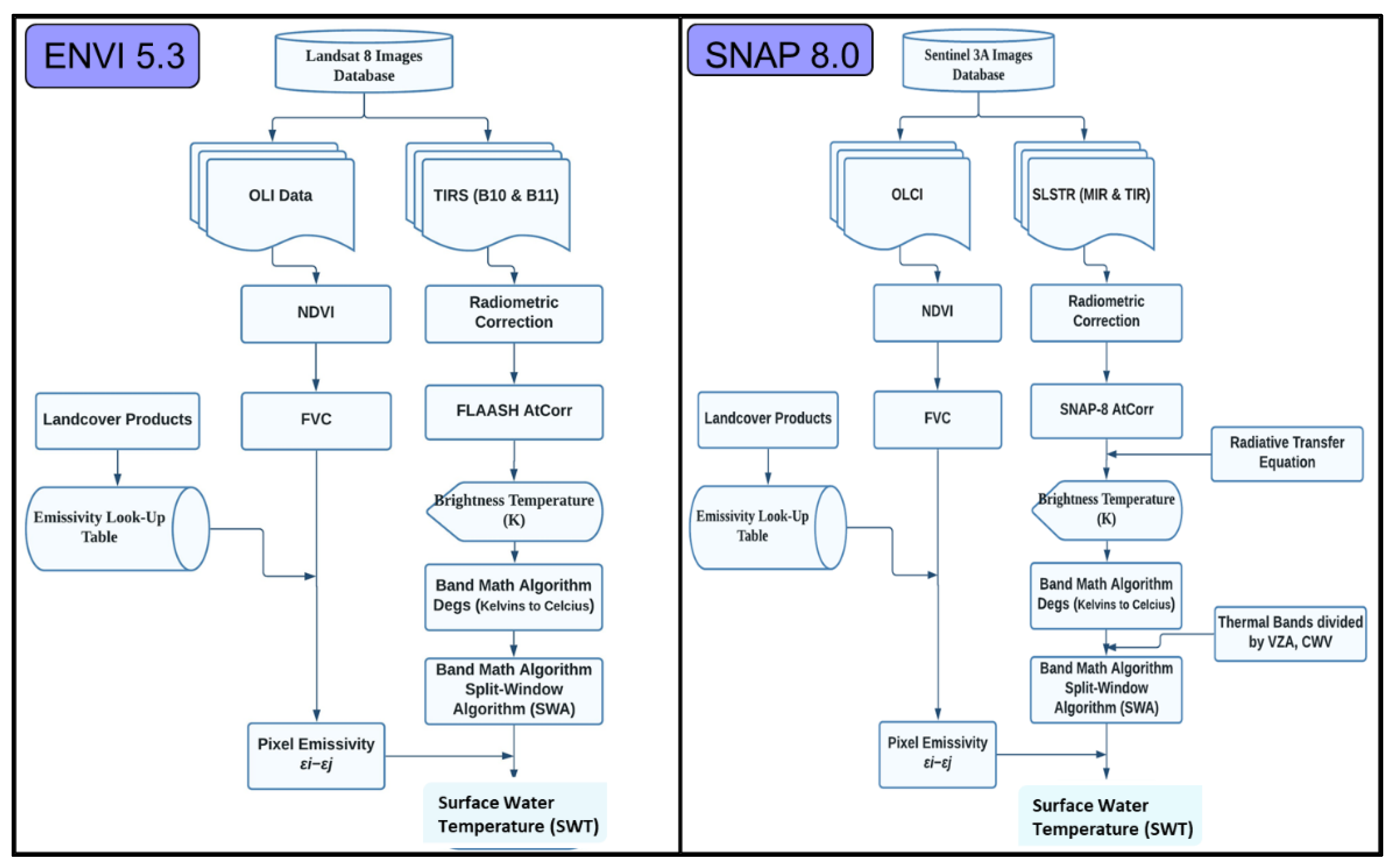
For S3A/B, SWT values were extracted from sea and land surface temperature radiometer (SLSTR) sensor level 2 land surface temperature (SLSTR L2) products. There are nine spectral bands on the SLSTR that are positioned within the 0.5–12 µm spectrum range. Furthermore, it consists of two additional channels for the recognition of fire; the visible-infrared bands and thermal-fire bands spatial resolutions are 500 m and 1 km, respectively. The algorithm is made up of five major steps: (1) radiometric image re-projection on the instrument grid, geometric correction which usually yields the level 1 SLSTR L1 re-gridding approach, and atmospheric correction; (2) the estimation of land surface emissivity (LSE) two methods of NDVI-THM and classification-based emissivity, (3) the NSW parameters presented by Sobrino and others [30], were used to estimate LST, and (4) validation of LST Sentinel-3 SLSTR LST product through comparison with in situ values [30]. Figure 2 depicts a flowchart to aid understanding of the step-by-step process for preprocessing of both L8 and S3 (Figure 2).

2.3. Machine and Deep Learning Algorithms Applied for Regression

This subsection is specifically for describing the theoretical background and all equations as well as defining all the quantities listed in the equations in order to organize and present the various ML/DL algorithms used in this study in the following order: Gaussian Process Regression (GPR), Support Vector Machine (SVM), Artificial Neural Network (ANN), Long-Short Term Memory (LSTM), and Convolutional LSTM (ConvLSTM). The listed ML/DL approaches were implemented in Python software version 3.6 using the NumPy, Pandas, and Matplotlib libraries, as well as the Statsmodels, Scikit-learn, and Statistica 13 packages for forecasting and data visualization. Additionally, the Statistica 13 software package was also used for hypothesis testing.
I.
Gaussian Process Regression (GPR)
The probabilistic machine learning models known as Gaussian Process Regressors (GPRs) are built on kernel functions and are similar to the Bayesian version of SVM models [31,32]. They are ideal models for resolving classification and regression prediction problems due to their computational efficiency [31,32]. GPR models often do not experience overfitting issues in contrast to ANNs [31,32]. Despite the benefits mentioned, researchers rarely use GPR models for hydrological and water resource modeling. The model can be mathematically expressed as follows using the notations form [33]:
Observation model:
( y | f ) , ϕ ~ i = 1 n p ( y i | f i , ϕ )  
GP prior:
f ( x ) | θ ~ gp ( m ( x ) ,   k ( x , x | θ ) )
Hyper prior:
θ , ϕ ~ p ( θ ) p ( ϕ )
where m ( x )   and   k ( x , x | θ ) indicate the mean and covariance functions and θ and Φ are parameters of the covariance function and the observation model, respectively. The joint distribution of training outputs (f) and test outputs ( f ¯ ) is given by:
[ f f ˜ ] | x , x ˜ , θ   ~   N ( 0 , [ K f , f K f , f ¯ K f ¯ ,   f K f ¯ , f ¯ ] )  
Marginal distribution of x ¯ as p( f ¯ | x ¯ ,θ) = N ( f ¯ |0, K f ¯ , f ¯ ) the conditional distribution of f ¯ (corresponding to test inputs x ¯ ) is:
f ˜ | f , x , x ˜ , θ   ~   N ( K f ¯ ,   f K f , f 1 f ,   K f ¯ , f ¯ K f ¯ ,   f K f , f 1 K f , f ¯ )
where K f , f ¯ = k(x, x ¯ |θ) and K f ¯ , f ¯ = k( x ¯ , x ¯ |θ)).
Different kernel functions can be used, including: quadratic, square d exponential, exponential, matern 5/2, matern 3/2, and their performances contrasted.
II.
Support Vector Machine (SVM)
Similar to GPR, SVM machine learning models have been successful in handling a variety of classification and regression problems. SVR is a nonparametric regression technique that creates a hyperplane with the lowest possible marginal error in order to construct correlations between predictor and response variables. It is based on the structural risk minimization theory [34]. The approximation function f(x) for an SVM model is denoted as follows for mapping training data of size n for input vector ((x1, …, xn) into output vector (y1, …, yn)) based on the learning function:
f ( x ) = i = 1 l ( α i α i )   K   ( x i , x ) + b  
where < x i , x > denotes the dot product of two vectors, x is the problem variable vector, b is the bias, α i α i are dual variables.
The radial basis function (RBF) is acknowledged in the literature as a superior kernel function [34,35]. Therefore, the Gaussian RBF is used as the kernel function for the SVM model in this study, which is based on empirical literature, and is defined as follows:
K   ( x i , x ) = e x p ( x x i 2 )
III.
Artificial Neural Network (ANN)
In contrast to SVM, ANN models use the assumption of minimizing empirical risk. Recently, multi-variate pattern classification and modeling of complicated environmental variables have dominated ANN research [36,37]. Simple ANNs consists of input layer(s), hidden layer(s), and one output layer and they are denoted by the basic function:
Y = f ( X ,   W ) +
where Y denotes the model’s response variables, X denotes its predictor variables, W denotes its weights, € denotes its bias term, and the function denotes the model’s functional relationship between its outputs, inputs, and parameters as mapped by an activation function. The network’s selected activation functions were the sigmoid function for the hidden layer and the rectified linear unit (ReLU) activation function for the output layer. In this study, three hidden layers and five input variables were used to predict the SWT.
IV.
Long Short Term Memory (LSTM)
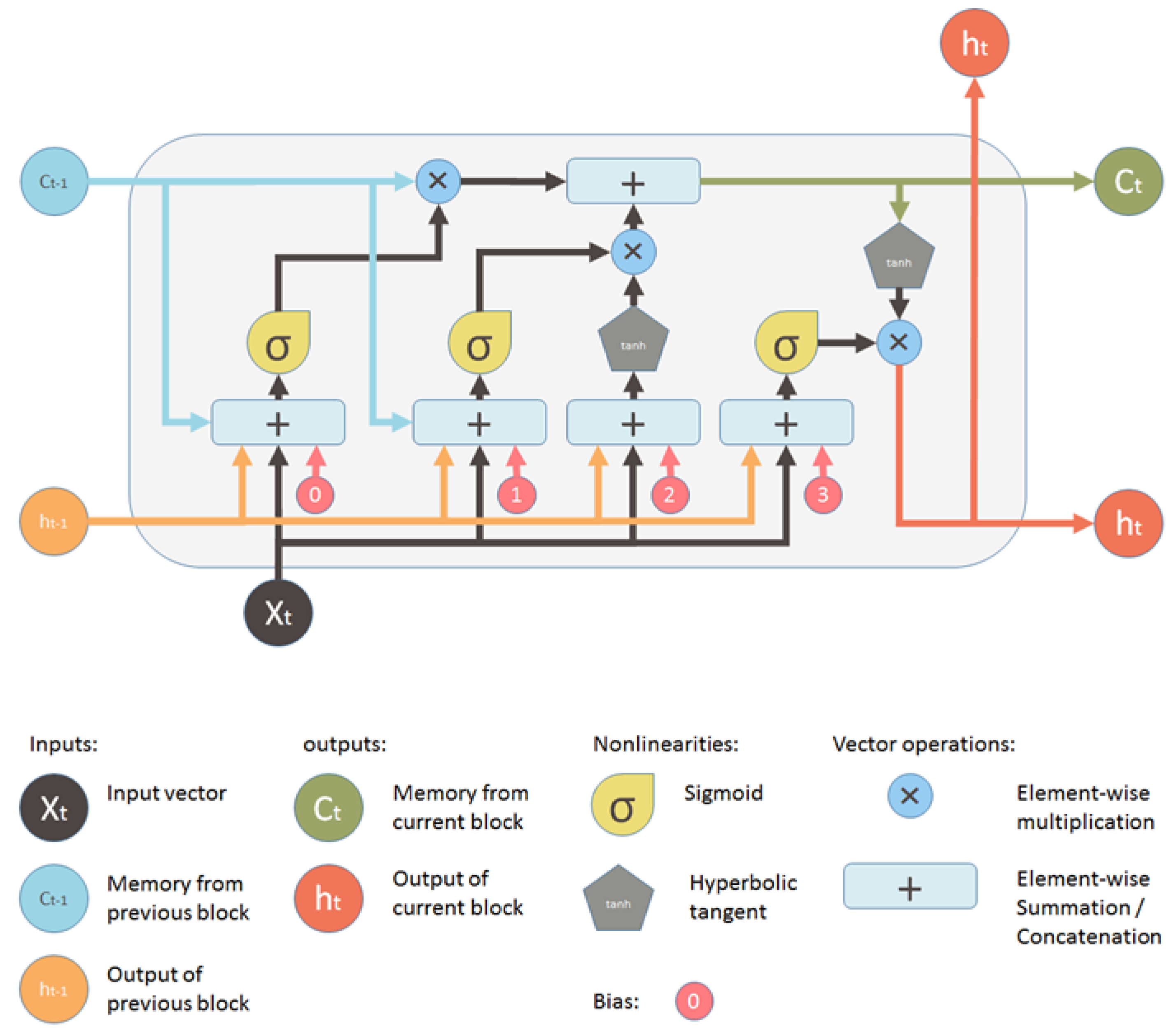
LSTM and gated recurrent units (GRUs) are recurrent neural network (RNN) variants [38]. However, LSTM and GRU maintain the advantage of memorizing long-term sequences by utilizing memory cells to store the activation value of previous data in the historical sequences. On the one hand, GRU preserves the benefits of LSTM for memorizing long-term sequences, while simplifying the architecture of the neural net, reducing training parameters, and mitigating the network’s over- and under-fitting problems, and it often outperforms LSTM in the scenarios of long text and small dataset [38]. On the other hand, regardless of LSTM high network complexity, which is frequently accompanied by over- and under-fitting, it provides increased flexibility to form ensemble learning methods for deep learning neural networks, such as convolutional LSTM (ConvLSTM) and combined full convolution LSTM (CFCC-LSTM) [39]. The ability to perform extensive feature engineering using ensemble deep learning networks is a useful application to high dimensional end-to-end spatiotemporal sequence prediction methods in satellite, which is why this study opted for an LSTM network over a GRU network [39]. Due to its capacity to learn on lengthy data sequences, while avoiding the inherent issues of gradient vanishing and explosion in RNN, LSTM outperforms RNN and GRU in lengthy time series predictions. An LSTM network has an input vector [h(t−1), x(t)] at time step t. The network cell state is denoted by c(t). The output vectors passing through the network between consecutive time steps t, t + 1 are denoted by h(t). The forget gate, input gate, and output gate are the three gates that make up an LSTM network and are used to update and control the cell states [38,39,40,41,42]. The gates are customized by hyperbolic tangent and sigmoid activation functions. On the assumption that new information would have entered the network, the forget gate directs that the information in a cell state be forgotten. Its output is computed by the function:
f t = σ ( W f [ h t 1 ,   x t ] )
On the basis of the new input information, the input gate controls how new information will be encoded into the cell state, and its output is indicated by the function:
i t = σ ( W i [ h t 1 ,   x t ] + b i )
The output gate regulates how data encoded in the cell state is transmitted back to the network (as the new input) input in the subsequent time step through the output vector h(t) [40,42]. The output gate’s activations are represented as:
o t = σ ( W o [ h t 1 , x t ] + b o )
and the cell’s output vector is given by:
h t = o t t a n h ( C t )
C t ˜ = t a n h ( W c [ h t 1 ,   x t ] + b c )
All of the steps are illustrated in Figure 3.
V.
Convolutional Long Short Term Memory (Conv-LSTM)
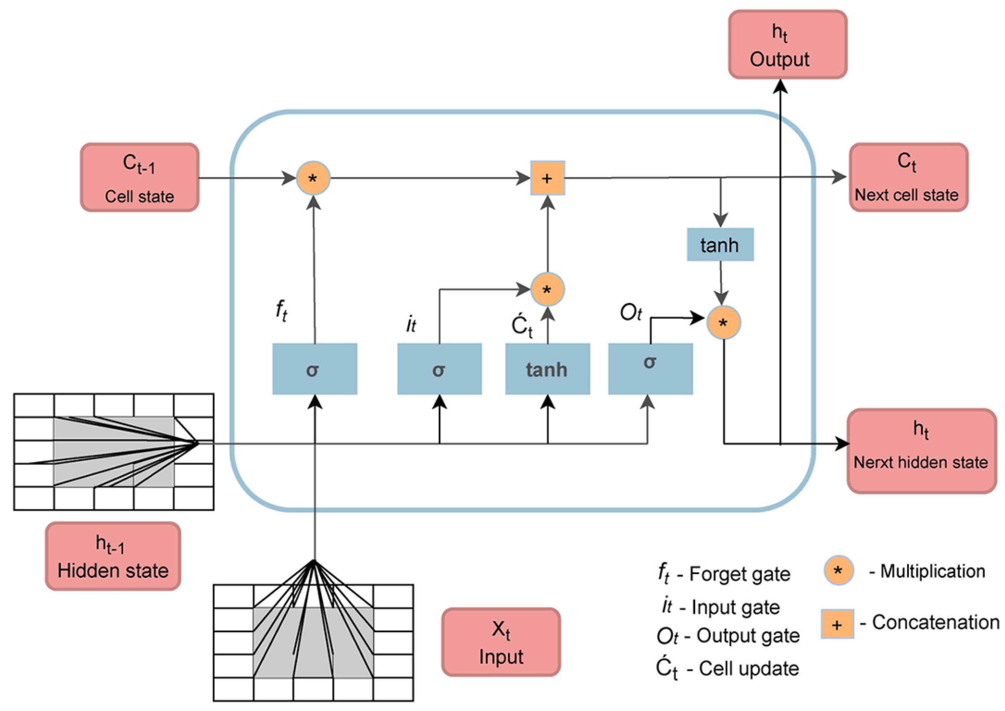
ConvLSTM is a type of recurrent neural network used for spatiotemporal prediction that incorporates convolutional structures in both input-to-state and state-to-state transitions [38,39]. Traditional RNN, GRU, LSTM, or CNN cannot fully exploit the temporal and spatial properties of open surface data using satellite images because data from various open surfaces water bodies is often spatially nonlinear and temporally dependent. Following that, the ConvLSTM algorithm was proposed to extend the capabilities of LSTM [43,44,45]. By using the inputs and past states of its local neighbors, the ConvLSTM predicts the future state of each cell in the grid. Using a convolution operator in the state-to-state and input-to-state transitions makes this is simple to accomplish (see Figure 4). The main equations of ConvLSTM are displayed below, where ∗ denotes the convolution operator and ⊙ the Hadamard product [38,39,45]:
i t = σ ( W x i X t + W h i H t 1 + W c i C t 1 + b i )
f t = σ ( W x f X t + W h f H t 1 + W c f C t 1 + b f )
C t = f t C t 1 + i t t a n h ( W x c X t + W h c t 1 + b c )  
o t = σ ( W x o X t + W h o t 1 + W c o C t + b o )
t = o t t a n h ( C t )
Sigmoid function:
σ ( x ) = 1 1 + e x
Tanh function:
t a n h = e x e x e x + e x
All steps and units are illustrated in Figure 4.

2.4. Sliding Window Time Series Cross-Validation and Model Evaluation Metrics

After successful application of all the regression models, the model performances were evaluated by measuring the following accuracy metrics: coefficient of determination (R2), root mean square error (RMSE), and uncertainties, i.e., bias-variance trade-off. To rigorously evaluate the performance of our proposed method, cross-validation was performed using the sliding window time series cross-validation (SWTSCV) method, which divided data into a series of overlapping training-testing sets [46]. As shown in Figure 5, each set is moved forward through the time series. SWTSCV is the most appropriate and robust evaluation method because it takes into account time indices and is capable of capturing autocorrelations. The principle is that the model should be trained using time series and its performance should be evaluated using (unseen) test data, which should always be the future data. Each model was evaluated on the test set, and the R2 and RMSE values were recorded. The SWTSCV-model scores were displayed using boxplots, and the average of the recorded and model errors were computed [47]. In our study, we used 10-time series split (i.e., i = 10). Time series cross-validation was selected because it is usually the most effective method for estimating the uncertainty in error statistics and gaining insight into the generalization ability of a model.

2.5. Performance Evaluation Metrics

This experiment compares the prediction accuracy of baseline ML to DL models presented under the machine learning section: GPR, SVR, ANN, LSTM, and 1D-ConvLSTM. Lee and Kim. [48] used Nash–Sutcliffe Efficiency (NSE) and RMSE as model performance evaluation metrics in a similar study. However, our model evaluation was based on (R2), RMSE, and bias-variance trade-offs. Mean absolute error (MAE) measures the extent to which a model is able to predict extreme events or outliers, such as extreme temperature heat wave or cold, and in this study MAE was not a useful metric because our data did not have extreme events or outliers as such.
R2 is a measure of how simulated variables can be predicted based on measured variables. Its strength ranging from 0 to 1, closer to 0 indicates a lower correlation, while close to 1 represents a high correlation.
R 2 = S S R S S T = [ i = 1 n ( y i y ¯ i ) ( y ^ i y ^ ¯ i ) ] 2 [ i = 1 n ( y i y ¯ i ) 2 i = 1 n ( y ^ i y ^ ¯ i ) 2 ]
RMSE is the standard deviation of the errors.
R M S E = 1 n i = 1 n ( y i y ^ i ) 2  
Bias is the mean error defined by the following function:
B i a s = 1 n i = 1 n ( y i y ^ i )  
where y ^ i and y i are the ith prediction and observation values, while y ¯ i and y ^ ¯ i are the calculated averages for the ith term observation and prediction values; and n is the total sample size for all data points. The higher the magnitude of R2 and the lower the RMSE, variance, and bias, the higher the model precision and accuracy for SWT, showing a better fit for the model predictions.

2.6. Hypothesis Testing (Two-Factor ANOVA) and Post-Hoc Scheffe

In this study, two different satellite sensors are applied, which affect model performances in different ways. Similarly, five different ML/DL algorithms are used and they affect model performance differently. Our research design allows us to focus on comparing three things: (1) how the different ML/DL models performed, (2) how the two satellites performed when compared to each other, and (3) how the effects of both the satellite used and ML/DL algorithm used affects model performance. Therefore, a two-factor ANOVA experimental design was adopted to test the following hypothesis:
H O :  
no main effects on model accuracy due to the type of satellite used (Factor 1)
H O :  
no main effects on model accuracy due to the type of ML/DL used (Factor 2)
H O :  
no interactive effects (Interaction) on model accuracy
In case of interactive effects between the two factors, the Scheffe method was used for a post-hoc comparison of the simple main effect. In the absence of interactive effects between the two factors, main effects were tested at α = 0.05 significance level.

3. Results

3.1. Descriptive Statistics

The descriptive statistics (sample size, mean, standard deviation, range, and inter-quartile range) for the in situ measured RH, WS, Precip, SWTGT, and the satellite derived SWT, i.e., SWTL8 and SWTS3 provide a summary of the data used in this study (Table 1). The historical data for in situ observations span a period of 28 years (January 1993 to 2020); however, the only matching satellite data and in situ observations spanned the years 2013 to 2020 due to the fact that L8 and S3 were operationalized during the years 2013 and 2016, respectively. We briefly outline some notable characteristics of our time series datasets before discussing model performances. In comparison to L8 (N = 882), sample size for S3 (N = 1050) was huge because S3 samples more frequently than L8, nearly once per day vs. twice a month. The range, median, and mean for L8’s estimated SWT were higher than those calculated by S3, indicating a difference in the two sensors’ levels of accuracy. There were no significant differences in the distribution of the other micro-climate data, as determined by the measure of central tendency scores as a result of all the data being measured and collected from the same meteorological station. There were no notable outliers, but shifting seasonal patterns allowed for the observation of seasonality as reflected in the cyclical maximum and minimum values of parameters, such as AAT, SWTGT, SWTL8, SWTS3, and P.

3.2. Long Term Atmospheric Air and Surface Water Temperature Trends for Mundan Water Reservoir (1993–2020)

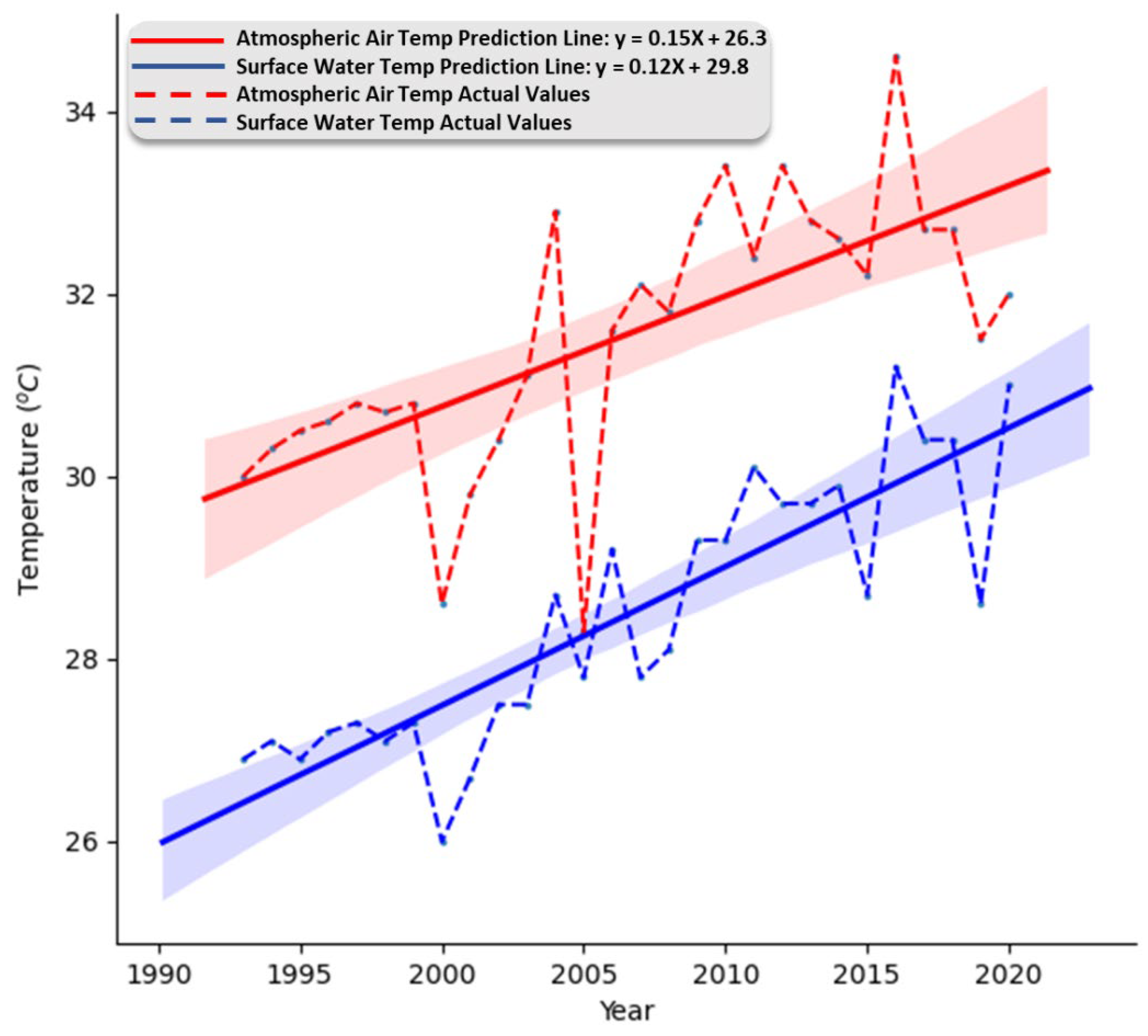
In the past 28 years, Taiwan EPA has collected data from SWT sampling points and station COR314; the results have shown a gradual but significant increase in both SWT and AAT around Mundan. Figure 6 depicts data recorded by the relevant authorities in the study area for almost three decades from 1993 to 2020. During the recorded period, both AAT and SWT for Mundan reservoir increased by 0.15 °C and 0.12 °C, respectively indicating warming temperatures in and around the Mundan Reservoir. As of 2006, the annual average atmospheric air temperature recorded was higher than the average (31.6 °C), and similarly, at the same time the annual average surface water temperature was higher than the average (28.5 °C). The trends for SWT and AAT are identical and they confirm a higher positive correlation (Figure 6). In fresh water ecosystems, photic zone water temperature measurements typically react quickly to brief changes in meteorological forcing, so that lake surface water essentially displays the same temperature signature as the surrounding air (see Figure 6). Surface water temperature generally mirrors rises in air temperature better than similar declines.

3.3. Exploratory Data Analysis–Correlation between Different Variables

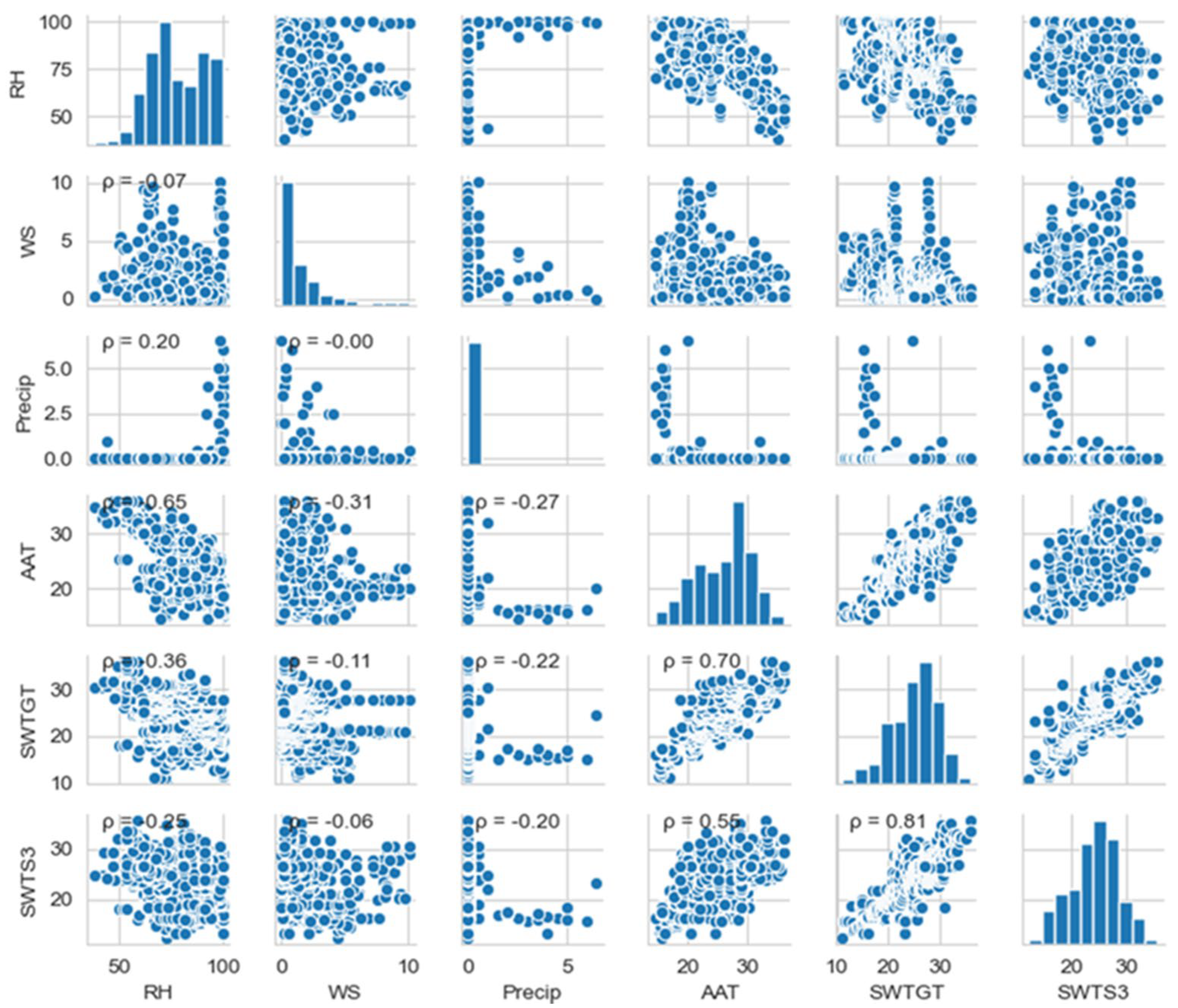
Pairwise multi-correlation analysis was performed on all variables used in this study, whether they were input or output variables (Figure 7). The resulting correlogram shows a combination of scatter plots (depicting a correlation between each pair of numerical variables) and histograms showing the distribution of each variable along the diagonal line. The thermodynamic exchanges between the reservoir boundary system and its surroundings, which is primarily atmospheric air, is responsible for the significant positive correlation between atmospheric air and surface water temperature (ρ = 0.70) [49]. Additional factors, such as secondary hydrological factors, i.e., snowmelt input, surface run-off, discharge, streambed including groundwater input being a key factor, and topography also contribute towards this thermodynamic exchange [50,51,52]. Therefore, it is imperative that research that evaluates the future impacts of warming water bodies consider changes in local hydrological and climatological factors. Similarly, satellite derived surface water temperature (SWTS3) showed strong positive correlations (ρ < 0.81) with SWTGT and (ρ = 0.55) AAT. However, there was a significant inverse relationship between relative humidity and SWTGT (ρ < −0.36), SWGS3 (ρ < −0.25), and AAT (ρ < −0.65). Except for its association with AAT (ρ < −0.31), wind speed’s correlation with other variables ranges from mildly negligible to low or no meaningful correlation.

3.4. Machine Learning Models

Three ML (GPR, SVM, ANN) and two DL-based models (LSTM, ConvLSTM) were selected for the test. SWTSCV was used to test both the train and test datasets. The grid-search range and selected hyperparameters of each ML method (GPR, SVR, ANN), as well as LSTM and ConvLSTM, are explained and highlighted in Table 2. The hyperparameter optimization was carried out in various ML/DL modules in the scikit-learn 0.20.3 Python v3.6 packages. Table 2 lists the grid-search hyperparameter optimization specifications for all of the models used.

4. Discussion

4.1. Factors Affecting the Accuracy of SWT Predictions

The accuracy of predictions in water quality parameters has been shown to depend on several factors that include but are not limited to the type of machine and deep learning modeling algorithms used [53,54,55], type of satellites used [56], and atmospheric correction methods applied [57]. However, no one factor has, up to this point, consistently provided optimal results in every situation. In a study reported by Arias-Rodriguez and others [55], who used cross-validation of machine learning algorithms to calculate Secchi Disk Depth (SDD) and turbidity estimates for the Valle de Bravo reservoir in central Mexico using MERIS data from 2002 to 2012 [55], the models did well estimating both parameters as reflected by excellent cross-validation (CV) scores. GPR performed better than the other models (SDD: R2 = 0.81; RMSE = 0.15; Turbidity: R2 = 0.86; RMSE = 0.95); the other models linear regression (LR), SVM, and random forest regressor (RFR) trailed behind. In another separate but similar study, water reflectance data obtained from both a hand-held spectroradiometer and satellite data was used to examine four ML approaches for retrieving three water quality parameters (Chl-a, SS, and turbidity) over the coastal waters of Hong Kong [53]. They also mapped the spatial distribution of these parameters. According to the results of cross-validation, ANN was able to reach the highest levels of accuracy for the water quality indicators for both in situ reflectance data (0.89 Chl-a, 0.93 SS, and 0.82 turbidity) and satellite data (0.91 Chl-a, 0.92 SS, and 0.85 turbidity). Further comparisons were made between the water quality characteristics retrieved by the ANN model and those retrieved by the standard C2RCC-Nets processing chain model for Case-2 Regional/Coast Color (C2RCC). The results of the standard Case-2 Regional/Coast Color (C2RCC) processing chain model C2RCC-Nets and the ANN model were further compared with station-based water quality data using a different set of satellite data. The potential of using ML and neural networks (NNs) for the retrieval of water quality metrics is demonstrated by all of the studies that have been cited [53]. This has only been applied to optically active and inactive water quality parameters. Our work expands the scope of this research to include thermal infrared channels for determining the thermal properties of surface water.
Our study demonstrates the following:
Water 14 02935 i001
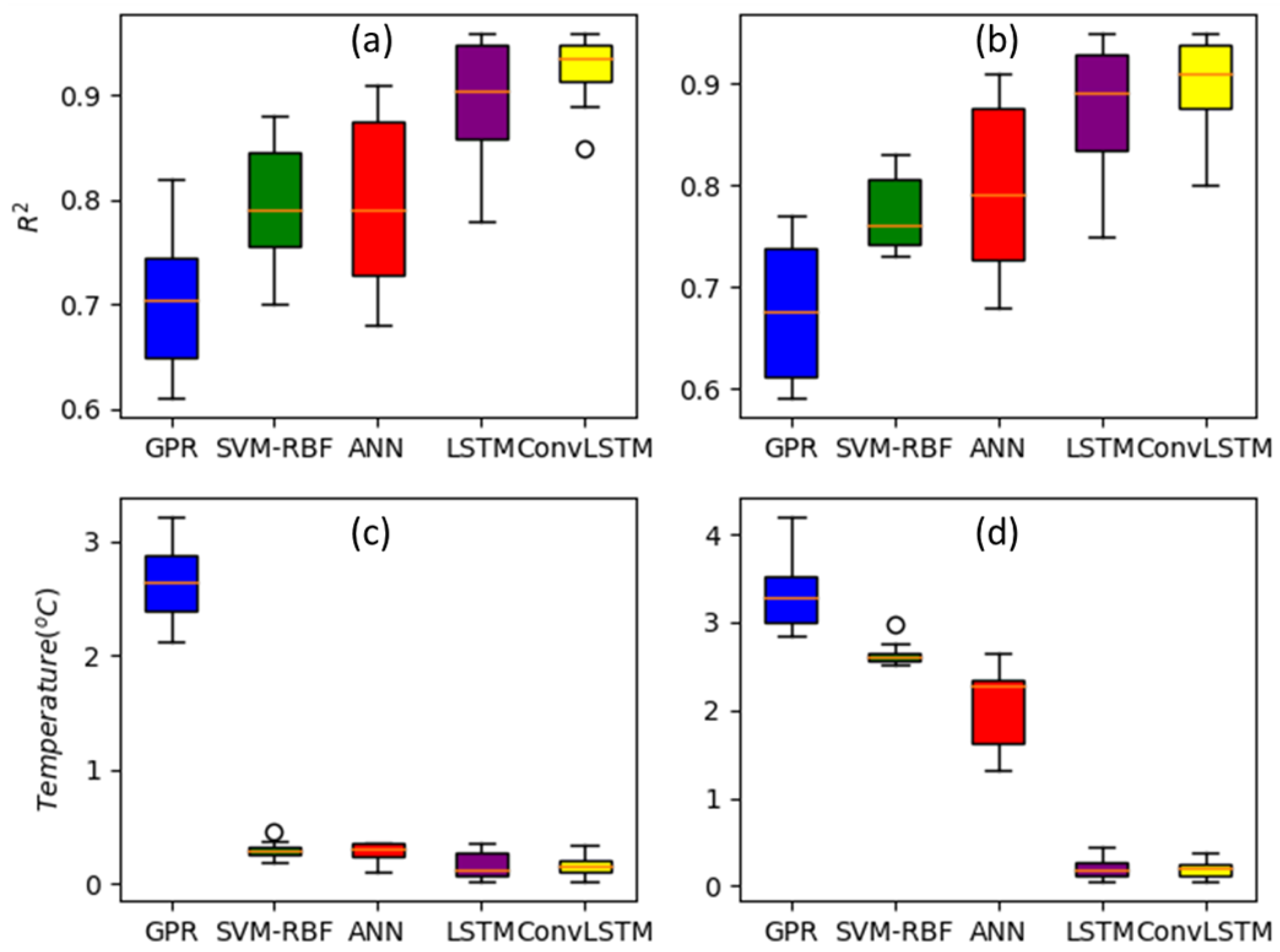
The five models tested performed well on both the test and training sets (accuracy > 0.67 for S3 and >0.71 for L8). Refer to Figure 8;
Water 14 02935 i001
DL models outperformed all other models in terms of greater R2 and as well as lower RMSE values when comparing the five generated models, achieving the highest accuracy in testing data. In terms of R2 and RMSE, 1D-ConvLSTM performed ahead of every other model for both satellites following the descending order: 1D-ConvLSTM > LSTM > ANN > SVM > GPR (Figure 8);
Water 14 02935 i001
Two deep-learning architectures (LSTM and 1D-ConvLSTM) performed relatively better than conventional and simple ANN architectures on test data used to evaluate different models. LSTM layers provide an added advantage over conventional model architecture when working with time series data since they are made up of memory cell blocks (known as hidden units in simple hidden layers). The hidden memory cell blocks can store information for longer time interval [58]. Deep-learning architectures needed more time to train than basic ML structures despite having superior predictive accuracy because they had more trainable parameters. Although adopting techniques, such as transfer learning or graphics processing unit (GPU) computing, can help to reduce training times;
Water 14 02935 i001
For all the evaluated models, the median R2 values ranged from 0.67 to 0.92, while the median RMSE scores ranged from 0.16 to 3.4 °C. In addition, L8 models performed better than their S3 corresponding models. It is also important to note that for both satellites, DL models performed better than conventional ML techniques. Similarly, this trend is also observed for the RMSE metric.
The type of satellite selected for the estimation of a water quality parameter is also a significant factor influencing the prediction accuracy since sensor-specific features, such as the spatial, spectral, and temporal resolutions of satellite imaging, affect the accuracy of mapping water quality. The importance of sensor selection in retrieval of water quality parameters is highlighted in a similar study that compared ground-truth SWT measurements to Landsat-5 Thematic Mapper (TM) and -7 Enhanced Thematic Mapper Plus (ETM+) derived SWT measurements [59], absolute errors were within acceptable 2 °C range, indicating that the Landsat algorithm is stable enough to determine seasonal trends and assess inter-annual variability of lake, reservoir, and estuarine temperatures. Several studies [56,60,61], also carried out an inter-sensor comparison through analyzing different spectral designs and resolutions of MultiSpectral Instrument (MSI) and Operational Land Imager (OLI) sensors and discussed the effects that the different sensor designs had on the performance of the sensors in retrieving Chlorophyll-a. Despite the fact that these studies compare different water quality parameters (Chlorophyll-a) and different sensors (OLI and MSI) to those used in this study, their relevance is that they explain how different sensors perform differently under specified conditions. Primarily, there are more bands in the MSI, particularly in the visible-near infrared area (three red-edge bands: 700–800 m). Additionally, some of these MSI bands, such as the green (3), red (4), and near infrared (8a) bands, have a finer spectral resolution. The spatial resolutions for the MSI are 10 m (4 bands), 20 m (6 bands), and 60 m (3 bands), but the spatial resolution for all the OLI bands is 30 m for all bands because thermal infrared bands (B10 and B11) can be resampled at 30m. Similar findings were achieved by other scientists who compared the performances of statistical models using these two sensors [61]. In all these cases, MSI showed superior performances over OLI and this can be attributed to finer spectral and higher spatio-temporal MSI resolution [60]. However, due to a lack of thermal IR bands, MSI is unable to monitor temperature. Sentinel-3 SLSTR, which carries 9 bands and can be applied for thermal and fire monitoring, was therefore used in this investigation. Data products for Sentinel-3 always remain freely available and accessible through the Copernicus Hub (https://scihub.copernicus.eu/ accessed on 31 July 2021), covering a large monitoring area and gathering satellite images once per day, despite the fact that it has a coarser spatial resolution. Only a few studies have been conducted to assess how well Sentinel-3 SLSTR products perform. In one such rare study, the Sentinel-3 SLSTR LST product was assessed in analyzing seasonal variations and to perform a separate inter-sensor comparison with MODIS [62]. The two LST datasets from Sentinel-3 and MODIS displayed the same pattern during seasonal variation. However, comparisons of sensor performance show that Sentinel-3 LST performed better overall and in all seasons. This study was designed to compare the performances of two distinct satellite sensors S3-SLSR and L8-TIRS for retrieval of SWT.
Our study demonstrates the following:
Water 14 02935 i001
Both performance assessment metric scores indicate that L8-TIRS outperformed S3-SLSR. According to the two line graphs in Figure 9, L8 has a lower RMSE than S3 for all models, while the opposite is true for R2 (refer to Figure 8);
Water 14 02935 i001
Furthermore, the results of the two sample t-tests confirm the null hypothesis (H0), which states that the average RMSE score for Landsat-8 is assumed to be less than or equal to the average of Sentinel-3’s RMSE score, with equal or pooled variance (p-value = 0.9453, (p(x ≤ T) = 0.05). This means that the probability of a type I error, which involves rejecting the correct H0, is too high: 94.53% for the 50 samples. This is further evidence that L8 SWT estimates are more precise than S3 estimates;
Water 14 02935 i001
These sensor performances may be attributed to the following factors: sensor characteristics, L8 has a higher spatial resolution compared to S3, data processing, season, day-night changes (in the case of Sentinel-3), and atmospheric correction.
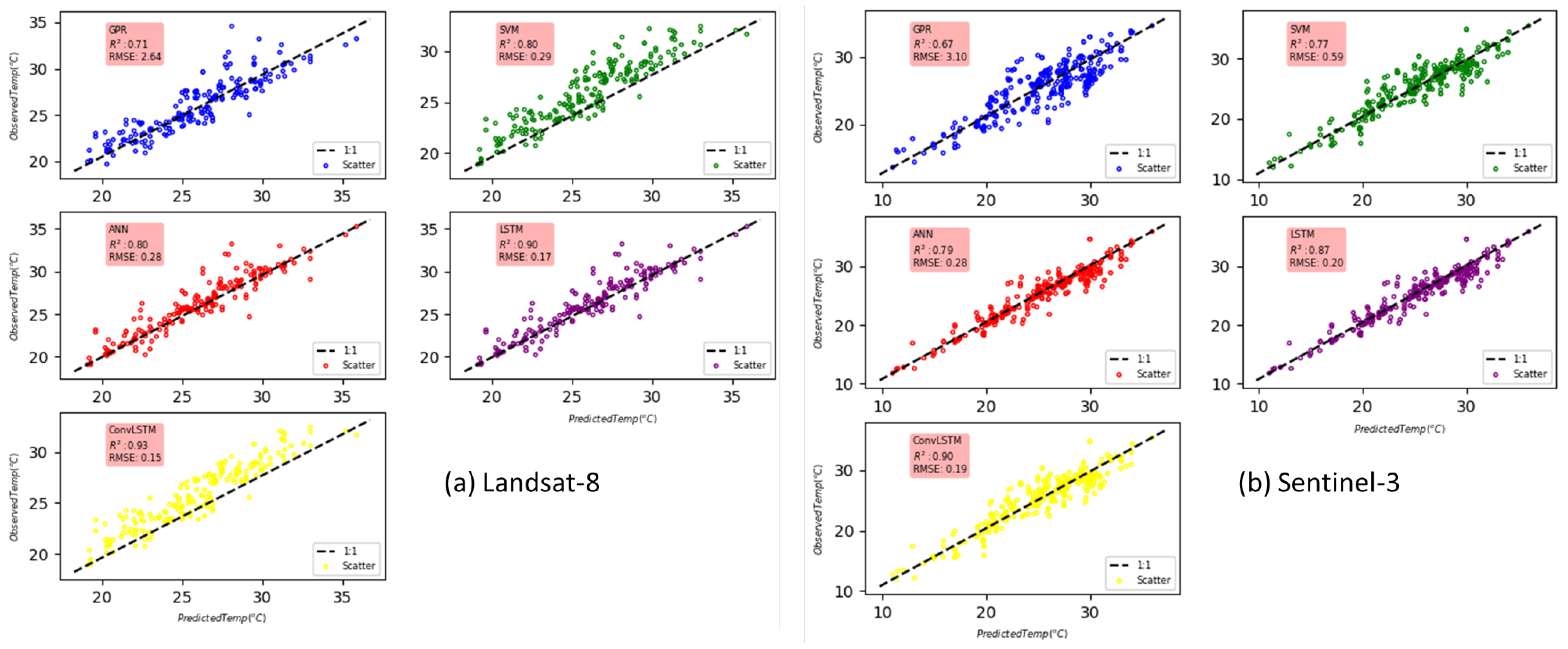
Scattergrams (Figure 9) were used as a simple way to visualize and evaluate model performance by regressing the observed SWT (in the y-axis) vs. predicted SWT (in the x-axis) and comparing how the different models performed using the slope and intercept parameters against the identity line (1:1) [63]. All the regression models showed a highly significant relation between predicted and observed SWT, a confirmation that the models performances were satisfactory. The scatter plots highlight average R2 and RMSE of every model in each subplot.

4.2. Hypothesis Testing: Two-Factor ANOVA

Every ML/DL model was subjected to a SWTSCV in Scikit-Learn, producing an array of ten scores for 10-time series splits. Since two satellites and six ML/DL models were used, this resulted in 12 groups with 10 RMSE scores per group. The two factors that were taken into consideration when designing a two-factor ANOVA experiment were satellite type and ML/DL type.
Our research demonstrated the following:
Water 14 02935 i001
Type of ML/DL main effect (F = 17.4607, p = 4.001 × 10⁻¹² ***);
Water 14 02935 i001
The satellite type main effect (F = 15.4478, p = 0.0001208 ***);
Water 14 02935 i001
Interaction effect (satellite type × type of ML/DL) (F = 3.5325, p = 0.008399 ***);
Water 14 02935 i001
The results indicate that both factors and their interaction have an impact on model performance;
Water 14 02935 i001
An increasing effect based on the factorial analysis of variance using effect size estimates ( η p 2 ) was observed in the following descending order: type of ML/DL > interaction > type of satellite;
Water 14 02935 i001
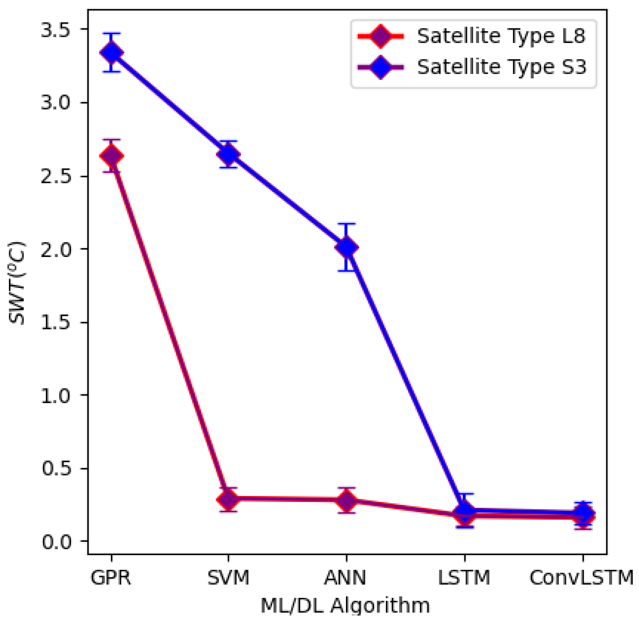
According to the two-factor ANOVA design approach, the selection of ML/DL is therefore more significant than the type of satellite used. The model score for S3 is improved by using DL models as shown by diverging or crossing lines, which shows evidence of interaction between the two factors (Figure 10);

4.3. Hypothesis Testing: Scheffe’s Post-Hoc Multiple Comparison

The main effects for both factors and their interactive effects are significant, therefore Scheffe’s post-hoc pairwise multiple comparison is used to identify group pair means that differ significantly. The highlights of the post hoc analysis show that pairwise group comparison between GPR (S3 and L8), SVM (S3 only), and ANN (S3 only) models for both showed significant differences with all other machine and deep learning models. In contrast, all the other pairwise comparisons did not exhibit statistical evidence of significant difference (Table 3).

4.4. Bias-Variance Trade-off for the ML/DL Models

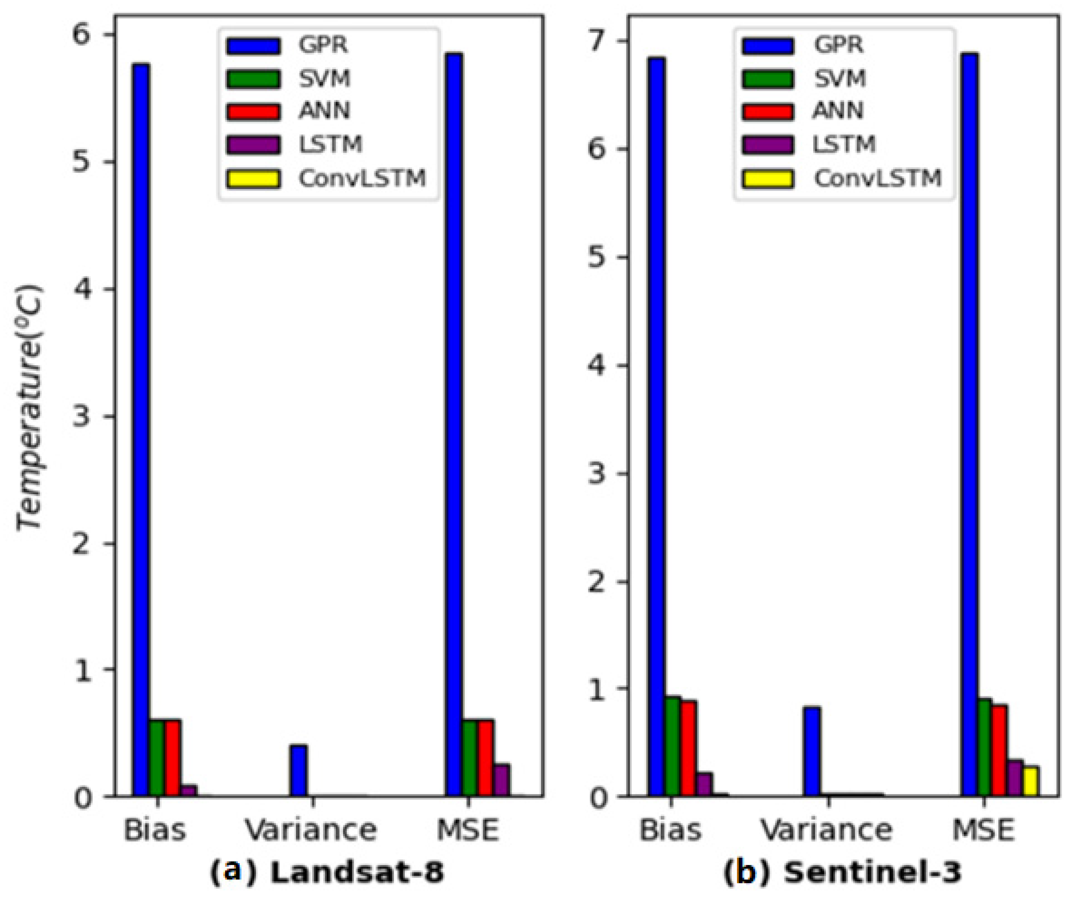
R2 is constrained in its utility as a validation metric score because high R2 does not always imply high accuracy if the estimates are significantly biased [64,65,66]. Nonetheless, it can frequently be applied as an assessment tool to evaluate the algorithm’s consistency across a range of measurements [64,65,66]. The limitation of RMSE estimates is that they do not capture the average error [49]. Therefore, to avoid potentially erroneous interpretations of R2 and RMSE, bias-variance decomposition of the error was used as a tool to simultaneously identify the bias errors (underfitting) and variance errors (overfitting) that prevent supervised learning algorithms from generalizing beyond their training sets. The GPR emerges for having inflated bias across all satellites (Figure 11), which can be explained by the fact that its simple model architecture fails to capture key data regularities, leading to underfitting. Similar to GPR, SVM and ANN are relatively low complexity models that are plagued by the same bias problem, the only difference is that the severity of their bias is significantly diminished. DL models are ideal for solving regression prediction problems for large data samples because, despite them being more complex models than ML, they nevertheless maintained lower bias and variance metrics (Figure 11), making them accurate and precise in determining SWT.

4.5. Spatio-Temoporary Variation Thermal Maps for Mundan

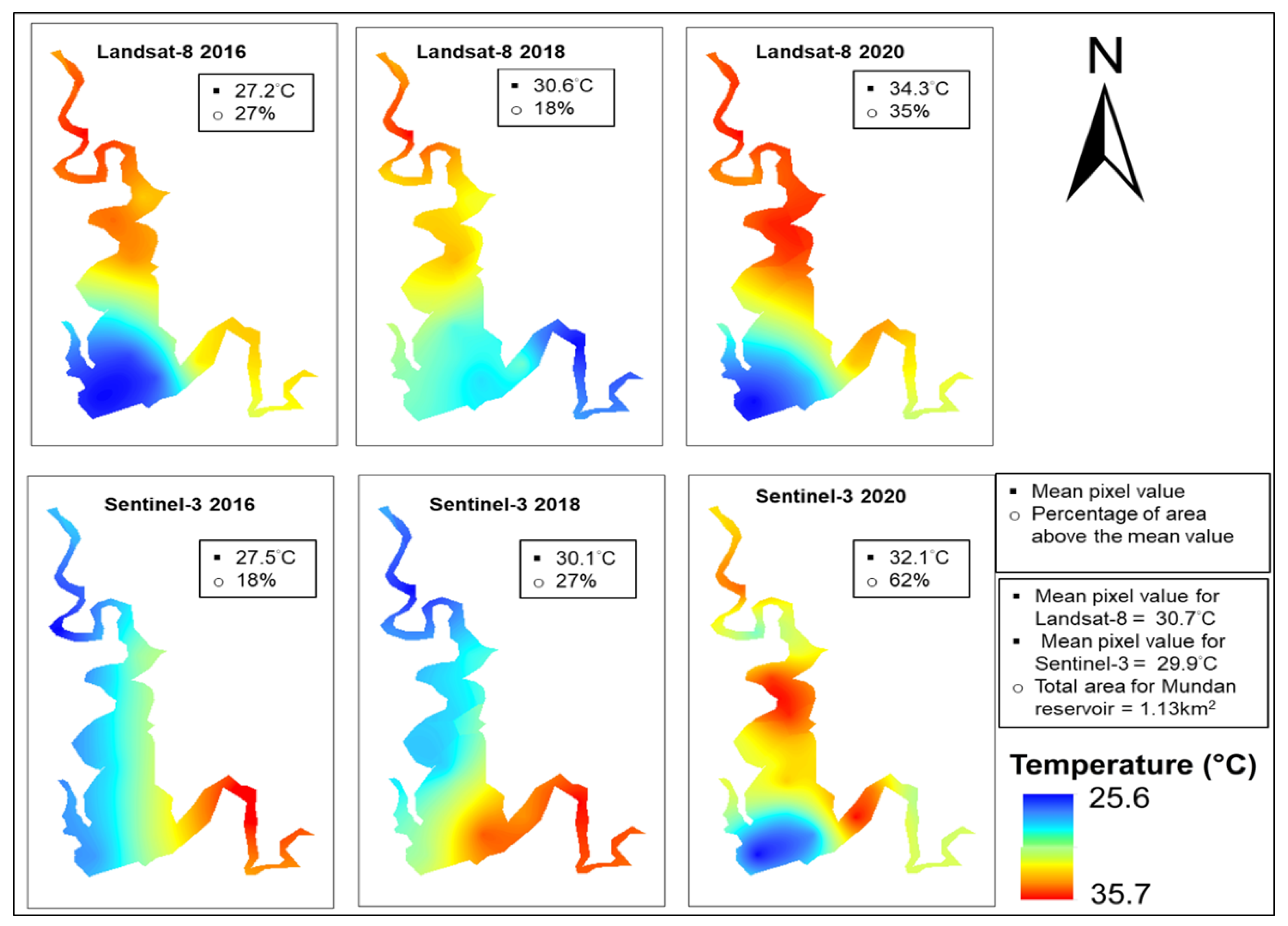
Based on L8 and S3 1D-ConvLSTM projections, SWT delineation maps show the spatial distribution of water temperature in Mundan Reservoir. The SWT geo-spatial distribution maps for the years 2016, 2018, and 2020 shows the average annual pixel temperature values calculated. The average annual pixel temperature values predicted using 1D-ConvLSTM for both satellites were plotted and to smoothen the inter-pixel values Kriging interpolation was used. The mean pixel temperature values for all the satellites show a noticeable increase from 2016 to 2020, while L8 SWT estimates are typically higher than S3 estimates (Figure 12). The Mundan Reservoir showed some differences in the pixel-to-pixel comparison between Landsat-8 and Sentinel-3 products of the corresponding years, with the exception of S3 2016 and 2018-pixel, temperature readings being higher in the northern parts of the reservoir (red and orange color). The disparity can be attributed to uncertainties, biases, and errors in monitoring small inland waters using various sensors, which are caused by a variety of factors [67,68]. These factors include complex optical water properties, surface glint, atmospheric aerosol heterogeneity, and the proximity of reflecting surfaces. Furthermore, radiation effects from the environment (adjacent effects) with complex geometry add to the difficulty, particularly for small inland lakes [19]. A combination of these factors makes obtaining accurate information on observed water systems difficult.
For all the satellites, there is a general increase in the area covered by pixels with temperatures above the mean pixel value, indicating that the reservoir is warming. The reservoir’s mean pixel values display rising temperatures and heat gain (orange). Hu [68] recommended that the sensor’s pixel size be at minimum four times more than the width of the surface slick being detected by the satellite. For the Mundan reservoir, which covers a total area of 1.13 km2, a full resolution projected satellite picture of Sentinel-3 resampled at 300 m × 300 m SLSR pixel theoretically yields 13 pixels. Under such circumstances, the accuracy of the results at specific sampling points is likely to be impacted by the effects of neighboring and adjacent pixels and an increased number of mixed pixels. For instance, an error resulting from the patchiness of sporadic blooms in water polluted by algal blooms [68,69]. In contrast, Landsat-8 TIRS pixels can be resampled at a resolution of 30 m × 30 m, covering 1111 pixels for the same 1.13 km2. Therefore, a sampling point is clearly discernable with minimum effects from its neighboring or adjacent pixels and has less mixed pixels overall. These are some of the possible underlying reasons behind the superior performances by L8.

5. Conclusions

Our research described the retrieval of SWT over Mundan Water Reservoir based on Sentinel-3A/B SLSTR and Landsat-8 TIRS sensors. Observations of long term temperature trends in Mundan Reservoir is indicating that the reservoir is experiencing warming. This combined together with the spatio-temporary SWT variation maps in Section 4.5 shows that water bodies are a good indicator of how climate change is affecting the aquatic ecosystems. To be specific, Mundan Reservoir surface water is warming at a rate of 0.12 °C per year and the warming rate of the AAT surrounding the reservoir area is 0.15 °C per year. We were successful in developing ML and DL models that explain potential sources of uncertainty relating to the spatial, spectral, and temporal resolutions of satellite images as well as how ML/DL model type affects SWT mapping in Mundan water reservoir. All of the models performed satisfactorily when tested against in situ measurements, with the largest error being a RMSE of 5 °C or less (RMSE < 5 °C) that was encountered by the worst performing GPR. The following conclusions can be noted as follows:
(1)
The ANOVA result demonstrated that the ML/DL model used had a more significant impact on estimation accuracy than the type of satellite used. However, it demonstrates that both factors had a significant impact in improving SWT’s estimation accuracy;
(2)
To further support this, DL models applied to low resolution satellites performed significantly well;
(3)
The considered important evaluation metrics for estimation of SWT were R2, RMSE, and bias-variance trade-off evaluators;
(4)
The maximum prediction accuracy was achieved by the ConvLSTM based on L8-TIRS data, with R2 = 0.93, RMSE = 0.15 °C.
This study’s successful implementation of the ConvLSTM algorithm to enhance the estimate performance of SWT to get even higher precision with low resolution sensors, such as Sentinel-3’s SLSR, is a significant contribution. Additionally, applying a DL model has demonstrated its ability to manage model uncertainties.

Author Contributions

Conceptualization, S.S.M. and J.-L.C.; methodology, S.S.M.; software, S.S.M. and J.-L.C.; validation, S.S.M. and J.-L.C.; formal analysis, S.S.M.; investigation, S.S.M.; resources, J.-L.C.; data curation, S.S.M.; writing—original draft preparation, S.S.M.; writing—review and editing, J.-L.C.; visualization, S.S.M.; supervision, J.-L.C.; project administration, J.-L.C.; funding acquisition, J.-L.C. All authors have read and agreed to the published version of the manuscript.

Funding

The National Pingtung University of Science and Technology (NPUST) in Taiwan’s department of Soil and Water Conservation, in collaboration with the department of Civil Engineering, funded this research.

Data Availability Statement

The USGS and ESA websites provide free access to primary data in the form of satellite images. Following formal approval of your request, you can access ground-truth data from the Taiwan EPA website. However, the corresponding author can also make all of the curated data used in this specific study available upon your request.

Acknowledgments

We gratefully acknowledge the Taiwan EPA, USGS, and ESA for providing us with free data for use in this study.

Conflicts of Interest

The authors declare no conflict of interest.

References

  1. Mansourmoghaddam, M.; Ghafarian Malamiri, H.R.; Rousta, I.; Olafsson, H.; Zhang, H. Assessment of Palm Jumeirah Island’s construction effects on the surrounding water quality and surface temperatures during 2001–2020. Water 2022, 14, 634. [Google Scholar] [CrossRef]
  2. Suzuki, H.; Nakatsugawa, M.; Ishiyama, N. Climate change impacts on stream water temperatures in a snowy cold region according to geological conditions. Water 2022, 14, 2166. [Google Scholar] [CrossRef]
  3. Ficklin, D.L.; Stewart, I.T.; Maurer, E.P. Effects of climate change on stream temperature, dissolved oxygen, and sediment concentration in the sierra Nevada in California. Water Resour. Res. 2013, 49, 2765–2782. [Google Scholar] [CrossRef]
  4. Ho, J.C.; Michalak, A.M.; Pahlevan, N. Widespread global increase in intense lake phytoplankton blooms since the 1980s. Nature 2019, 574, 667–670. [Google Scholar] [CrossRef]
  5. Findlay, H.S.; Turley, C. Ocean acidification and climate change. In Climate Change; Elsevier: Amsterdam, The Netherlands, 2021; pp. 251–279. [Google Scholar] [CrossRef]
  6. The Food and Agriculture Organization of the United Nations (FAO); The International Water Management Institute (IWMI). Water Pollution from Agriculture: A global Review. FAO: Rome, Italy; International Water Management Institute (IWMI): Colombo, Sri Lanka. CGIAR Research Program on Water, Land and Ecosystems 2017, (WLE). Available online: https://www.fao.org/3/i7754e/i7754e.pdf (accessed on 20 June 2021).
  7. Damania, R.; Desbureaux, S.; Rodella, A.-S.; Russ, J.; Zaveri, E. Quality Unknown: The Invisible Water Crisis; World Bank Publications: Washington, DC, USA, 2019. [Google Scholar] [CrossRef]
  8. Cherif, E.K.; Mozetič, P.; Francé, J.; Flander-Putrle, V.; Faganeli-Pucer, J.; Vodopivec, M. Comparison of in-situ chlorophyll-a time series and sentinel-3 ocean and land color instrument data in Slovenian National Waters (gulf of trieste, Adriatic Sea). Water 2021, 13, 1903. [Google Scholar] [CrossRef]
  9. Zhu, W.-D.; Qian, C.-Y.; He, N.-Y.; Kong, Y.-X.; Zou, Z.-Y.; Li, Y.-W. Research on chlorophyll-a concentration retrieval based on BP neural network model—case study of Dianshan Lake, China. Sustainability 2022, 14, 8894. [Google Scholar] [CrossRef]
  10. Seidel, M.; Hutengs, C.; Oertel, F.; Schwefel, D.; Jung, A.; Vohland, M. Underwater use of a hyperspectral camera to estimate optically active substances in the water column of Freshwater Lakes. Remote Sens. 2020, 12, 1745. [Google Scholar] [CrossRef]
  11. Yang, H.; Kong, J.; Hu, H.; Du, Y.; Gao, M.; Chen, F. A review of remote sensing for Water Quality Retrieval: Progress and challenges. Remote Sens. 2022, 14, 1770. [Google Scholar] [CrossRef]
  12. Malakar, N.K.; Hulley, G.C.; Hook, S.J.; Laraby, K.; Cook, M.; Schott, J.R. An operational land surface temperature product for landsat thermal data: Methodology and validation. IEEE Trans. Geosci. Remote Sens. 2018, 56, 5717–5735. [Google Scholar] [CrossRef]
  13. Kumar, C.; Podestá, G.; Kilpatrick, K.; Minnett, P. A machine learning approach to estimating the error in satellite sea surface temperature retrievals. Remote Sens. Environ. 2021, 255, 112227. [Google Scholar] [CrossRef]
  14. Ai, B.; Wen, Z.; Jiang, Y.; Gao, S.; Lv, G. Sea surface temperature inversion model for infrared remote sensing images based on Deep Neural Network. Infrared Phys. Technol. 2019, 99, 231–239. [Google Scholar] [CrossRef]
  15. Sammartino, M.; Buongiorno Nardelli, B.; Marullo, S.; Santoleri, R. An artificial neural network to infer the Mediterranean 3D chlorophyll-a and temperature fields from remote sensing observations. Remote Sens. 2020, 12, 4123. [Google Scholar] [CrossRef]
  16. Jung, S.; Yoo, C.; Im, J. High-resolution seamless daily sea surface temperature based on satellite data fusion and machine learning over Kuroshio Extension. Remote Sens. 2022, 14, 575. [Google Scholar] [CrossRef]
  17. Barth, A.; Alvera-Azcárate, A.; Licer, M.; Beckers, J.-M. DINCAE 1.0: A convolutional neural network with error estimates to reconstruct sea surface temperature satellite observations. Geosci. Model Dev. 2020, 13, 1609–1622. [Google Scholar] [CrossRef]
  18. Hafeez, S.; Wong, M.S.; Abbas, S.; Asim, M. Evaluating landsat-8 and sentinel-2 data consistency for high spatiotemporal inland and coastal water quality monitoring. Remote Sens. 2022, 14, 3155. [Google Scholar] [CrossRef]
  19. Pan, Y.; Bélanger, S.; Huot, Y. Evaluation of atmospheric correction algorithms over lakes for high-resolution multispectral imagery: Implications of adjacency effect. Remote Sens. 2022, 14, 2979. [Google Scholar] [CrossRef]
  20. Malenovský, Z.; Rott, H.; Cihlar, J.; Schaepman, M.E.; García-Santos, G.; Fernandes, R.; Berger, M. Sentinels for science: Potential of sentinel-1, -2, and -3 missions for scientific observations of ocean, cryosphere, and land. Remote Sens. Environ. 2012, 120, 91–101. [Google Scholar] [CrossRef]
  21. Torres, R.; Snoeij, P.; Geudtner, D.; Bibby, D.; Davidson, M.; Attema, E.; Potin, P.; Rommen, B.Ö.; Floury, N.; Brown, M.; et al. Gmes sentinel-1 mission. Remote Sens. Environ. 2012, 120, 9–24. [Google Scholar] [CrossRef]
  22. Kravitz, J.; Matthews, M.; Lain, L.; Fawcett, S.; Bernard, S. Potential for high fidelity global mapping of common inland water quality products at high spatial and temporal resolutions based on a synthetic data and machine learning approach. Front. Environ. Sci. 2021, 9, 587660. [Google Scholar] [CrossRef]
  23. Caballero, I.; Roca, M.; Santos-Echeandía, J.; Bernárdez, P.; Navarro, G. Use of the Sentinel-2 and Landsat-8 Satellites for Water Quality Monitoring: An Early Warning Tool in the Mar Menor Coastal Lagoon. Remote Sens. 2022, 14, 2744. [Google Scholar] [CrossRef]
  24. Dorji, P.; Fearns, P. Impact of the spatial resolution of satellite remote sensing sensors in the quantification of total suspended sediment concentration: A case study in turbid waters of northern Western Australia. PLoS ONE 2017, 12, e0175042. [Google Scholar] [CrossRef] [PubMed]
  25. Al-Kharusi, E.S.; Tenenbaum, D.E.; Abdi, A.M.; Kutser, T.; Karlsson, J.; Bergström, A.-K.; Berggren, M. Large-scale retrieval of coloured dissolved organic matter in Northern Lakes using sentinel-2 data. Remote Sens. 2020, 12, 157. [Google Scholar] [CrossRef]
  26. Yu, Z.; Yang, K.; Luo, Y.; Shang, C.; Zhu, Y. Lake surface water temperature prediction and changing characteristics analysis—a case study of 11 natural lakes in Yunnan-Guizhou Plateau. J. Clean. Prod. 2020, 276, 122689. [Google Scholar] [CrossRef]
  27. Yang, L.; Driscol, J.; Sarigai, S.; Wu, Q.; Lippitt, C.D.; Morgan, M. Towards Synoptic Water Monitoring Systems: A Review of AI Methods for Automating Water Body Detection and Water Quality Monitoring Using Remote Sensing. Sensors 2022, 22, 2416. [Google Scholar] [CrossRef]
  28. Du, C.; Ren, H.; Qin, Q.; Meng, J.; Zhao, S. A practical split-window algorithm for estimating land surface temperature from Landsat 8 data. Remote Sens. 2015, 7, 647–665. [Google Scholar] [CrossRef]
  29. Wan, Z.; Dozier, J. A generalized split-window algorithm for retrieving land-surface temperature from space. IEEE Trans. Geosci. Remote Sens. 1996, 34, 892–905. [Google Scholar] [CrossRef]
  30. Sobrino, J.A.; Li, Z.-L.; Stoll, M.P.; Becker, F. Multi-channel and multi-angle algorithms for estimating sea and land surface temperature with ATSR data. Int. J. Remote Sens. 1996, 17, 2089–2114. [Google Scholar] [CrossRef]
  31. Cui, T.; Pagendam, D.; Gilfedder, M. Gaussian process machine learning and Kriging for groundwater salinity interpolation. Environ. Model. Softw. 2021, 144, 105170. [Google Scholar] [CrossRef]
  32. Ewusi, A.; Ahenkorah, I.; Aikins, D. Modelling of total dissolved solids in water supply systems using regression and supervised machine learning approaches. Appl. Water Sci. 2021, 11, 13. [Google Scholar] [CrossRef]
  33. Rasmussen, C.E. Gaussian processes in machine learning. Adv. Lect. Mach. Learn. 2004, 3176, 63–71. [Google Scholar] [CrossRef]
  34. Mamun, M.; Lee, S.-J.; An, K.-G. Temporal and spatial variation of nutrients, suspended solids, and chlorophyll in Yeongsan Watershed. J. Asia-Pac. Biodivers. 2018, 11, 206–216. [Google Scholar] [CrossRef]
  35. Mamun, M.; Kim, J.-J.; Alam, M.A.; An, K.-G. Prediction of algal chlorophyll-a and water clarity in monsoon-region reservoir using machine learning approaches. Water 2019, 12, 30. [Google Scholar] [CrossRef]
  36. Cho, K.H.; Sthiannopkao, S.; Pachepsky, Y.A.; Kim, K.-W.; Kim, J.H. Prediction of contamination potential of groundwater arsenic in Cambodia, Laos, and Thailand using Artificial Neural Network. Water Res. 2011, 45, 5535–5544. [Google Scholar] [CrossRef] [PubMed]
  37. Park, Y.; Cho, K.H.; Park, J.; Cha, S.M.; Kim, J.H. Development of early-warning protocol for predicting chlorophyll-a concentration using machine learning models in freshwater and estuarine reservoirs, Korea. Science of The Total Environment 2015, 502, 31–41. [Google Scholar] [CrossRef]
  38. Zhang, Z.; Pan, X.; Jiang, T.; Sui, B.; Liu, C.; Sun, W. Monthly and Quarterly Sea Surface Temperature Prediction Based on Gated Recurrent Unit Neural Network. J. Mar. Sci. Eng. 2020, 8, 249. [Google Scholar] [CrossRef]
  39. Yang, Y.; Dong, J.; Sun, X.; Lima, E.; Mu, Q.; Wang, X. A CFCC-LSTM model for sea surface temperature prediction. IEEE Geosci. Remote Sens. Lett. 2018, 15, 207–211. [Google Scholar] [CrossRef]
  40. Ye, W.; Zhang, F.; Du, Z. Machine Learning in Extreme Value Analysis, an Approach to Detecting Harmful Algal Blooms with Long-Term Multisource Satellite Data. Remote Sens. 2022, 14, 3918. [Google Scholar] [CrossRef]
  41. Jia, X.; Ji, Q.; Han, L.; Liu, Y.; Han, G.; Lin, X. Prediction of Sea Surface Temperature in the East China Sea Based on LSTM Neural Network. Remote Sens. 2022, 14, 3300. [Google Scholar] [CrossRef]
  42. Yan, S. Understanding LSTM and Its Diagrams. Medium. Available online: https://blog.mlreview.com/understanding-lstm-and-its-diagrams-37e2f46f1714 (accessed on 5 September 2022).
  43. Su, H.; Jiang, J.; Wang, A.; Zhuang, W.; Yan, X.-H. Subsurface Temperature Reconstruction for the Global Ocean from 1993 to 2020 Using Satellite Observations and Deep Learning. Remote Sens. 2022, 14, 3198. [Google Scholar] [CrossRef]
  44. Song, T.; Wei, W.; Meng, F.; Wang, J.; Han, R.; Xu, D. Inversion of Ocean Subsurface Temperature and Salinity Fields Based on Spatio-Temporal Correlation. Remote Sens. 2022, 14, 2587. [Google Scholar] [CrossRef]
  45. Iskandaryan, D.; Ramos, F.; Trilles, S. Bidirectional convolutional LSTM for the prediction of nitrogen dioxide in the city of Madrid. PLoS ONE 2022, 17, e0269295. [Google Scholar] [CrossRef] [PubMed]
  46. Kaastra, I.; Boyd, M. Designing a neural network for forecasting financial and Economic Time Series. Neurocomputing 1996, 10, 215–236. [Google Scholar] [CrossRef]
  47. Mozaffari, L.; Mozaffari, A.; Azad, N.L. Vehicle speed prediction via a sliding-window time series analysis and an evolutionary least learning machine: A case study on san francisco urban roads. Eng. Sci. Technol. Int. J. 2015, 18, 150–162. [Google Scholar] [CrossRef]
  48. Lee, S.; Kim, J. Predicting inflow rate of the Soyang River Dam using Deep learning techniques. Water 2021, 13, 2447. [Google Scholar] [CrossRef]
  49. McCombie, A.M. Some relations between air temperatures and the surface water temperatures of Lakes. Limnol. Oceanogr. 1959, 4, 252–258. [Google Scholar] [CrossRef]
  50. Webb, B.W.; Zhang, Y. Spatial and seasonal variability in the components of the river heat budget. Hydrol. Processes 1997, 11, 79–101. [Google Scholar] [CrossRef]
  51. Mohseni, O.; Stefan, H.G. Stream temperature/air temperature relationship: A physical interpretation. J. Hydrol. 1999, 218, 128–141. [Google Scholar] [CrossRef]
  52. Ficklin, D.L.; Luo, Y.; Stewart, I.T.; Maurer, E.P. Development and application of a hydroclimatological stream temperature model within the soil and water assessment tool. Water Resour. Res. 2012, 48. [Google Scholar] [CrossRef] [Green Version]
  53. Hafeez, S.; Wong, M.; Ho, H.; Nazeer, M.; Nichol, J.; Abbas, S.; Tang, D.; Lee, K.; Pun, L. Comparison of machine learning algorithms for retrieval of water quality indicators in case-II waters: A case study of hong kong. Remote Sens. 2019, 11, 617. [Google Scholar] [CrossRef]
  54. Ewuzie, U.; Bolade, O.P.; Egbedina, A.O. Application of deep learning and machine learning methods in water quality modeling and prediction: A Review. In Current Trends and Advances in Computer-Aided Intelligent Environmental Data Engineering; Elsevier: Amsterdam, The Netherlands, 2022; pp. 185–218. [Google Scholar] [CrossRef]
  55. Arias-Rodriguez, L.F.; Duan, Z.; Sepúlveda, R.; Martinez-Martinez, S.I.; Disse, M. Monitoring water quality of Valle de Bravo Reservoir, Mexico, using entire lifespan of Meris data and machine learning approaches. Remote Sens. 2020, 12, 1586. [Google Scholar] [CrossRef]
  56. Bande, P.; Adam, E.; Elbasit, M.A.A.; Adelabu, S. Comparing Landsat 8 and sentinel-2 in mapping water quality at Vaal dam. In Proceedings of the International Geoscience and Remote Sensing Symposium (IGARSS), Valencia, Spain, 22–27 July 2018; pp. 22–27. [Google Scholar]
  57. Windle, A.E.; Evers-King, H.; Loveday, B.R.; Ondrusek, M.; Silsbe, G.M. Evaluating atmospheric correction algorithms applied to olci sentinel-3 data of Chesapeake Bay Waters. Remote Sens. 2022, 14, 1881. [Google Scholar] [CrossRef]
  58. Baek, S.-S.; Pyo, J.; Chun, J.A. Prediction of water level and water quality using a CNN-LSTM combined deep learning approach. Water 2020, 12, 3399. [Google Scholar] [CrossRef]
  59. Schaeffer, B.A.; Iiames, J.; Dwyer, J.; Urquhart, E.; Salls, W.; Rover, J.; Seegers, B. An initial validation of Landsat 5 and 7 derived surface water temperature for U.S. lakes, reservoirs, and estuaries. Int. J. Remote Sens. 2018, 39, 7789–7805. [Google Scholar] [CrossRef]
  60. Pizani, F.M.; Maillard, P.; Ferreira, A.F.; de Amorim, C.C. Estimation of water quality in a reservoir from sentinel-2 MSI and landsat-8 oli sensors. ISPRS Ann. Photogramm. Remote Sens. Spat. Inf. Sci. 2020, V-3-2020, 401–408. [Google Scholar] [CrossRef]
  61. Yadav, S.; Yamashiki, Y.; Susaki, J.; Yamashita, Y.; Ishikawa, K. Chlorophyll estimation of lake water and coastal water using landsat-8 and sentinel-2a satellite. Int. Arch. Photogramm. Remote Sens. Spat. Inf. Sci. 2019, XLII-3/W7, 77–82. [Google Scholar] [CrossRef]
  62. Zarei, A.; Shah-Hosseini, R.; Ranjbar, S.; Hasanlou, M. Validation of non-linear split window algorithm for land surface temperature estimation using sentinel-3 satellite imagery: Case study; Tehran Province, Iran. Adv. Space Res. 2021, 67, 3979–3993. [Google Scholar] [CrossRef]
  63. Piñeiro, G.; Perelman, S.; Guerschman, J.P.; Paruelo, J.M. How to evaluate models: Observed vs. predicted or predicted vs. observed? Ecol. Model. 2008, 216, 316–322. [Google Scholar] [CrossRef]
  64. Ali, K.A.; Moses, W.J. Application of a PLS-augmented ANN model for retrieving chlorophyll-a from hyperspectral data in case 2 waters of the western basin of Lake Erie. Remote Sens. 2022, 14, 3729. [Google Scholar] [CrossRef]
  65. Seegers, B.N.; Stumpf, R.P.; Schaeffer, B.A.; Loftin, K.A.; Werdell, P.J. Performance metrics for the assessment of Satellite Data Products: An ocean color case study. Opt. Express 2018, 26, 7404. [Google Scholar] [CrossRef]
  66. Brewin, R.J.W.; Sathyendranath, S.; Müller, D.; Brockmann, C.; Deschamps, P.-Y.; Devred, E.; Doerffer, R.; Fomferra, N.; Franz, B.; Grant, M.; et al. The Ocean Colour Climate Change Initiative: III. A round-robin comparison on in-water bio-optical algorithms. Remote Sens. Environ. 2015, 162, 271–294. [Google Scholar] [CrossRef]
  67. Fisher, T.; Gibson, H.; Liu, Y.; Abdar, M.; Posa, M.; Salimi-Khorshidi, G.; Hassaine, A.; Cai, Y.; Rahimi, K.; Mamouei, M. Uncertainty-aware interpretable deep learning for slum mapping and monitoring. Remote Sens. 2022, 14, 3072. [Google Scholar] [CrossRef]
  68. Hu, C. A novel ocean color index to detect floating algae in the global oceans. Remote Sens. Environ. 2009, 113, 2118–2129. [Google Scholar] [CrossRef]
  69. Shen, M.; Chen, J.; Zhuan, M.; Chen, H.; Xu, C.-Y.; Xiong, L. Estimating uncertainty and its temporal variation related to global climate models in quantifying climate change impacts on hydrology. J. Hydrol. 2018, 556, 10–24. [Google Scholar] [CrossRef]
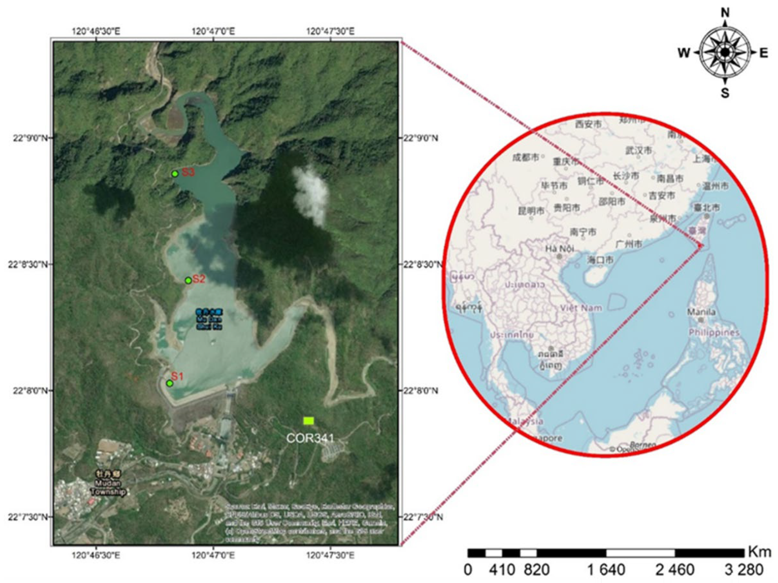
Figure 1. Location of Mundan water reservoir and Mundan meteorological station (COR 341) with respect to the map of Taiwan, the reservoir is showing the sampling points S1–S3 as indicated on the map (left-side).
Water 14 02935 g001
Figure 2. Workflow to show the process of retrieval of SWT from L8 and S3 images by ENVI 5.3 and SNAP 8.0 software respectively.
Water 14 02935 g002
Figure 3. LSTM building block units redrawn from Yan. S. Medium Review article [42].
Water 14 02935 g003
Figure 4. Diagram of a ConvLSTM cell structure from Iskandaryan and others [45].
Water 14 02935 g004
Figure 5. Graphic presentation of sliding window time series cross-validation.
Water 14 02935 g005
Figure 6. Trends in annual atmospheric and surface water temperatures recorded by the Mundan microclimate weather station and the Taiwan EPA, respectively, 1993–2021.
Water 14 02935 g006
Figure 7. Correlation matrix for the different variables highlighting pairwise numerical value of ρ, scatterplots, while the diagonal bar charts represent a data distribution pattern for each variable.
Water 14 02935 g007
Figure 8. Distribution of SWTSCV performance metric evaluation scores, 10-R2, and RMSE scores for each algorithm because the sliding windows were split into 10-time series splits. The subplots column (a,c) are R2 and RMSE for L8, similarly (b,d) shows the same for S3.
Water 14 02935 g008
Figure 9. Observed vs. predicted WST regression scattergrams derived from the ML/DL models test data. The name of the ML/DL, R2 and RMSE are shown in the graph legends. The distribution of the scatter point markers along the line of equality (1:1) are also visualized in the figure; (a) Landsat-8 models are in the left and middle left columns, and (b) Sentinel-3 models are in the middle right and right columns.
Water 14 02935 g009
Figure 10. Line plots showing the outcome of a two factor experiment main and interactive effects of satellite type and type of ML/DL.
Water 14 02935 g010
Figure 11. Bias-Variance Trade-offs and MSE bar charts for all the models: (a) L8, and (b) S3 models.
Water 14 02935 g011
Figure 12. Time series for the spatial distribution of SWT based on ConvLSTM predictions smoothened by Kriging interpolation in Mundan water reservoir.
Water 14 02935 g012
Table 1. Descriptive statistics for all the input variables to the data of the models from 1993–2020.
Landsat-8 Data Set
IndexRH (%)WS (m/s)Precip (mm)AAT (°C)SWTL8 (°C)SWTGT (°C)
Count (N)882882882882882882
Mean66.81.420.1027.427.726.0
Std. Dev19.61.340.664.313.693.75
Min10001719.119.1
First Quartile57.30.3023.624.723
Median691027.62725.9
Third Quartile802.403130.328.7
Max997.7536.937.636.3
Sentinel-3 Data Set
IndexRH (%)WS (m/s)Precip (mm)AAT (°C)SWTS3 (°C)SWTGT (°C)
Count (N)105010501050105010501050
Mean77.91.390.0726.024.125.1
Std. Dev13.31.820.494.734.234.55
Min380014.412.411
First Quartile670.102221.221.7
Median760.8027.024.425.5
Third Quartile901.9029.12728.2
Max10010.16.53635.536
Notes: RH–Relative Humidity, WS–Wind Speed, Precip–Precipitation, AAT–Atmospheric Air Temperature, SWTS3 –Sentinel-3 Surface Water Temperature, SWTGT–Surface Water Temperature Ground Truth, SWTL8 –Landsat-8 Surface Water Temperature.
Table 2. Grid-search range of the parameters of each ML/DL method with test values for the hyper-parameters are sorted in ascending order.
ModelHyper-Parameter NameHyperparameter DescriptionGrid Search Parameter ValuesOptimal Hyper-Parameter Value
GPRlength_scaleThe length-scale of the respective feature dimension is specified.0.5, 1, 2, 31
Kernel functionTransforms data that is linearly inseparable into data that is linearly separable and specifies the kernel type to be used in the algorithm.RBF, Constant, and exponentialRBF
n_restarts_optimizerThe number of optimizer restarts required to find the kernel parameters that maximize the log-marginal likelihood.5, 7, 9, 11, 139
SVMCost (C)Regularization parameter0.1, 1, 10, 100, 100010
gammaKernel coefficient for RBF, poly and Sigmoid0.0001, 0.001, 0.01, 0.1, 10.0001
Kernel functionTransformation of linearly inseparable data to linearly separable ones and specifying the kernel type to be used in the algorithmRBF, Sigmoid, Linear, and PolynomialRBF
epsilon (ε)Defines a tolerance margin in which errors are not penalized.0.01, 0.1, 1, 1.50.1
ANNActivation functionsThe activation function compute the input values of a layer into output valuesReLU, Sigmoid, Softplus, and tanhSigmoid–hidden layers and ReLU–output layer
OptimizerThe optimizer changes the learning rate and weights of neurons in the neural network to achieve lowest loss functionAdam, SGD, RMSprop, and AdagradAdam
Learning rateLearning rate manipulates the step size for a model to attain the minimum loss function0.001, 10.01
NeuronsThe number of neurons in every layer is set to be the same and should be adjusted to the solution complexity10, 10065
EpochsThe number of times a whole dataset is passed through the neural network model 20, 100100
Batch sizeBatch size is the number of training data sub-samples for the input.50, 500100
Drop outDropout is another regularization layer. The dropout layer, randomly drops a certain number of neurons in a layer0, 20.9
Dropout rateThe rate of how much percentage of neurons to drop is set in the dropout rate0, 0.50.15
Batch NormalizationThe batch normalization layer normalizes the values passed to it for every batch. This is similar to standard scaler in conventional Machine Learning0, 10.90
LSTMLearning rateLearning rate controls the step size for a model to reach the minimum loss function0.001, 110−3
EpochsThe number of times a whole dataset is passed through the neural network model 20, 100100
Batch sizeBatch size is the number of training data sub-samples for the input.50, 500100
Drop outThe dropout layer is another name for the regularization layer, which randomly drops a set number of neurons in a layer.0, 20.5
ConvLSTMLearning rateLearning rate controls the step size for a model to reach the minimum loss function0.001, 110−3
EpochsThe number of times an entire dataset is processed through the neural network model.20, 100100
Batch sizeBatch size is the number of training data sub-samples for the input.50, 500100
Drop outThe dropout layer is another name for the regularization layer, which randomly drops a set number of neurons in a layer.0, 20.5
Table 3. Post-Hoc Scheffe test p-values for all 12 groups’ two level factors (Satellite Type * ML Algorithm) for RMSE.
L8L8L8L8L8L8S3S3S3S3S3S3
SLTML/DLGPRSVM-RBFSVM-LinANNLSTMConvLSTMGPRSVM-RBFSVM-LinANNLSTMConvLSTM
L8GPR
L8SVM-RBF0.001
L8SVM-Lin0.0011.00000
L8ANN0.0010.89999471.00000
L8LSTM0.0010.89999471.000000.8999947
L8ConvLSTM0.0010.89999471.000000.89999470.8999947
S3GPR0.0010.0010.000000.0010.0010.001
S3SVM-RBF0.89999470.0010.0000000.0010.0010.0010.001
S3SVM-Lin0.89999470.0010.0000000.0010.0010.0010.0010.00000
S3ANN0.0010.010.010.0010.0010.0010.0010.0011.00000
S3LSTM0.0010.89999470.89999470.89999470.89999470.89999470.0010.0010.9997810.001
S3ConvLSTM0.0010.89999470.89999470.89999470.89999470.89999470.0010.0010.9999740.0010.8999947
Notes: p-value figures highlighted in blue and red color indicate p *** < 0.001 and p ** < 0.01, respectively. Error; Between MS = 0.07129, df = 108.
Publisher’s Note: MDPI stays neutral with regard to jurisdictional claims in published maps and institutional affiliations.