Article

Land-Use and Land Cover Is Driving Factor of Runoff Yield: Evidence from A Remote Sensing-Based Runoff Generation Simulation

1
College of Urban and Environmental Sciences, Peking University, No. 5 Yiheyuan Road, Haidian District, Beijing 100871, China
2
Chemical Science College, Bordeaux University, UMR EPOC CNRS 5805, 33400 Talence, France
*
Author to whom correspondence should be addressed.
Water 2022, 14(18), 2854; https://doi.org/10.3390/w14182854
Submission received: 18 July 2022 / Revised: 7 September 2022 / Accepted: 8 September 2022 / Published: 13 September 2022

Abstract

:
The spatial distribution of water storage capacity has always been the critical content of the study of saturation-excess runoff. Xin’anjiang model uses the water storage capacity curve (WSCC) to characterize the distribution of water storage capacity for runoff yield calculation. However, the mathematical and physical foundations of WSCC are unclear, which is impossible to simulate runoff generation with complex basins accurately. To fill this gap, we considered the dominant role of basin physical characteristics in water storage capacity and developed a new integrated approach to solve the spatial distribution of water storage capacity (L-WSCC) to account for the spatiotemporal dynamics of their impact on runoff generation. The main contribution of L-WSCC was to confer WSCC more physical meaning and the spatial distribution of water storage capacity was explicitly represented more accurately, so as to better express the runoff generation and provide a new approach for runoff yield calculation in non-data basin. L-WSCC was applied to Misai basin in China and promising results had been achieved, which verified the rationality of the method (the mean Nash–Sutcliffe efficiency (NSE):0.86 and 0.82 in daily and hourly scale, respectively). Compared with WSCC, the performance of L-WSCC was improved (mean NSE: 0.82 > 0.78, mean absolute value of flood peak error (PE): 12.74% < 21.66%). Moreover, the results of local sensitivity analyses demonstrated that land-use and land cover was the major driving factor of runoff yield (the change of mean absolute error (ΔMAE): 131.38%). This work was significant for understanding the mechanisms of runoff generation, which can be used for hydrological environmental management and land-use planning.

Graphical Abstract

1. Introduction

Floods are the most common and highly destructive natural disaster in the world [1,2,3,4]. According to relevant research, the annual casualties caused by floods over the world exceed 50% of the total natural disasters, and the economic losses exceed 30% [5,6]. With the population surging and the acceleration of urbanization, the frequency of extreme rainfall events has become higher and higher, and the frequency, intensity, loss and the ranges of impact of flood disasters have shown a significant upward trend [7,8]. China is one of the countries with the most serious flood disasters in the world, and the flooding issues have become a comprehensive problem that cannot be ignored in the sustainable development [9]. Therefore, it is urgent to implement reasonable and scientific flood management measures to minimize the damage caused by floods.
Accurate runoff simulation is essential for flood management and plays a vital role in sustainable water resources management in reducing losses caused by flood disasters [2,10,11,12,13]. Water storage capacity curve (WSCC) is the key to the calculation of saturation-excess runoff and is applied to describe the distribution of basin water storage capacity for runoff simulation [14]. WSCC is represented by empirical Generalized Pareto Distribution, which has been extensively applied worldwide for a wide range of watershed scales, hydrology environmental conditions, flood simulation, and provides a scientific way to analyze the process of rainfall-runoff [15,16,17,18].
Although the WSCC method performs well in humid and subhumid regions for nature basins, it cannot characterize its connection to the internal characteristics of the basin due to its empirical origins [19,20,21,22]. This limitation causes that it performs only fairly even poorly in complex basins: the findings of Jayawardena et al. suggested that WSCC is less effective for runoff simulation in wet and dry transition seasons [23]; Zhuo et al. found that the soil moisture schemes of WSCC are generally not realistic in comparison with the reality [24]. Bartlett et al. pointed out that WSCC does not describe the spatial and temporal variability of runoff, which limited its application [25,26]. In addition, studies also showed that WSCC may fail to capture the vertical partial runoff [27]. These poor performances may be due to the WSCC method assuming a uniform basin with spatially uniform runoff processes [28]. Moreover, the WSCC method also lacks a description of the spatial variability of runoff and the physical meaning of WSCC is not clear enough, which is a generalized model [29,30]. This generalization ignores the influence of underlying surface changes on runoff yield [31,32,33]. Hence, when WSCC is applied to complex basins, significant errors can and do occur when calculating runoff yield.
To move beyond the limitations of the WSCC method, the related research have been done to study the relationship between the WSCC and related physical factors based on the sufficient remote sensing data [19,27]. Among them, water storage capacity and land-use types were strongly correlated because landscape had significant impacts on soil physical properties [34,35]. In vegetation region, many studies had been undertaken and the results showed that vegetation structures such as leaf area index, vegetation rooting depth, root depth, vegetation coverage and canopy density would profoundly affect water storage capacity [36,37,38,39,40]. Additionally, the effects of topography and terrain on water storage capacity were of great concern [25,30,41,42,43,44]. A significant number of studies had tried to calculate the water storage capacity using topographic index [22,45,46], slope [19,47,48], and elevation [30]. Furthermore, many studies evaluated the soil characteristics such as soil type [25], soil texture [30], soil wetness index [49], soil layer depth [29], soil hydraulic characteristics [19], soil moisture [50], soil humidity, and soil wetness [51], on water storage capacity to represent the soil water availability [30,52,53,54]. The effect of watershed area on water storage capacity was also studied [19,55].
As can be seen from the above studies, the WSCC is most closely associated with land-use, topography, soil, and vegetation. Consequently, many scholars have described the spatial distribution of water storage capacity based on these factors to produce a more reasonable runoff generation response: the results of Yao et al. showed that the water storage capacity of a basin can be derived by the soil texture and vegetation type [30]. Wang et al. solved the spatial distribution of water storage capacity through the relationship between the soil wetting ratio and the storage index, and achieved good outcome [56]. Guo et al. studied the water storage capacity based on topographic index and incomplete beta distribution and the results showed the new method produced a more reasonable runoff simulation [57]. Moreover, Gao et al.’s research in 404 watersheds showed that the spatial distribution of water storage capacity is the result of the combined effect of remote sensing factors such as slope, land-use, soil, and topography [19].
Although there have been many studies on the spatial distribution of water storage capacity, these studies have only conducted research from a certain aspect. No method has been proposed to solve the spatial distribution of water storage capacity by integrating various remote sensing factors to date. Moreover, no report quantified the influence of each factor on the runoff yield. To fill this gap, a comprehensive method considering various factors for spatial distribution of water storage capacity based on abundant remote sensed data was proposed in our study, called L-WSCC. The L-WSCC has physical basis in a spatial distribution of water storage capacity that is derived from distributions of spatially heterogeneous variables such as land-use, terrain geomorphology, and soil. The object of the paper is to construct a physics-based water storage capacity method through various remote sensing factors to improve the physical basis of the original empirical WSCC. L-WSCC can provide a new representation of the runoff generation, so as to extend the traditional WSCC with a spatial characterization of runoff variability. In addition, this paper also quantitatively assessed which factors dominated the impact on runoff yield and how much it accounted for. It was expected that the proposed method could enhance the physical meaning of WSCC to improve its runoff simulation capability.

2. Materials and Methods

2.1. Study Area and Data Collection

In this study, Misai watershed was employed as study area. It is a complex forest watershed located in Quzhou city, Zhejiang Province, China, with an area of 797 km2 (29.1°–30.0° N, 118.0°–119.0° E) (Figure 1a). Its altitude varies between 105 m and 1253 m, and the overall terrain decreases from northwest to southeast (Figure 1b). The watershed has one major tributary, Majinxi, one of the sources of the Qiantang River (Figure 1b). Misai watershed belongs to the mid-subtropical zone and has frequent monsoon activities. This region has a mean annual temperature of 17 °C, with average minimum and maximum temperatures of 12.9 °C and 21.3 °C, respectively [58]. The climate is humid with an average annual rainfall from 1500 mm to 2000 mm. 60% of the rainfall occurs during short heavy rainfall in summer. The humic acrisols (FAO soil classification, ACu) soil is the main soil type and the soil moisture within 200 cm is about 352.80 kg/m2 (https://ldas.gsfc.nasa.gov/gldas/, accessed on 9 November 2021). The watershed is rich in forest resources, accounting for 86.3% of the area, including woodland, shrub forest, and sparse woodland.
Flood disasters have occurred frequently in this region. According to statistics, flood disasters of varying degrees occurred in the region (big floods in 1955, 1969, and 1999) and the flood disasters of 2006 and 2017 were highly devastating, which caused heavy loss on property and society [59,60]. It is, therefore, of great importance to investigate the hydrological regime in this region. The study area is chosen because of the threat of flooding and its compliance with the saturation-excess runoff.
The hydrological data used in this paper mainly come from 6 hydrological observation stations (included 6 rainfall stations, 1 runoff observation station and 1 evaporation station) (Figure 1b), including rainfall, evaporation, and runoff data (daily data) and 17 floods data (hourly data) (Table S1).
The remote sensing data used in this paper mainly include DEM data, Landsat data (land cover data), soil data, and vegetation type map. The DEM data set is provided by Geospatial Data Cloud site, Computer Network Information Center, Chinese Academy of Sciences (http://www.gscloud.cn, accessed on 9 November 2021). Five different resolutions are obtained through resampling: 30 m, 100 m, 200 m, and 500 m to study the change of sub-grid so as to weaken the scale influence as much as possible (see Section 2.3). The corresponding terrain information (relief, slope, and aspect) are shown in Figure S1. Landsat satellite data are taken from NASA website (https://earthexplorer.usgs.gov, accessed on 9 November 2021). Seven phases of TM/MSS satellite images with less than 10% cloud cover were obtained. The synthesis time of the image is about June of 1982–1988. Based on remote sensing images, the land-use classification of the study area is obtained through supervised classification. The land-use map is shown in Supplementary Materials (Figure S2). The results are shown in Table S2. The data of soil types comes from the global soil data released by FAO, which is in accordance with the FAO/UNESCO System of Soil Classification. The distribution of soil types is shown in Figure S3a. The vegetation data are from the vegetation map of the people’s Republic of China (1:1,000,000). The vegetation area of the study area accounts for a large proportion, mainly conifer and broadleaved mixed forests, which are mainly located in the northern mountainous area (Figure S3b).

2.2. WSCC and L-WSCC

The WSCC is the main form of calculating runoff yield in saturation-excess runoff. It is the cumulative frequency curve of part of the area varying with the storage capacity and represents the surface distribution of water storage capacity of the basin [14]. Rainfall-runoff relationships can be obtained through WSCC. According to experience and experimental data, the WSCC is parabolic usually. Please see Text S1 for more details.
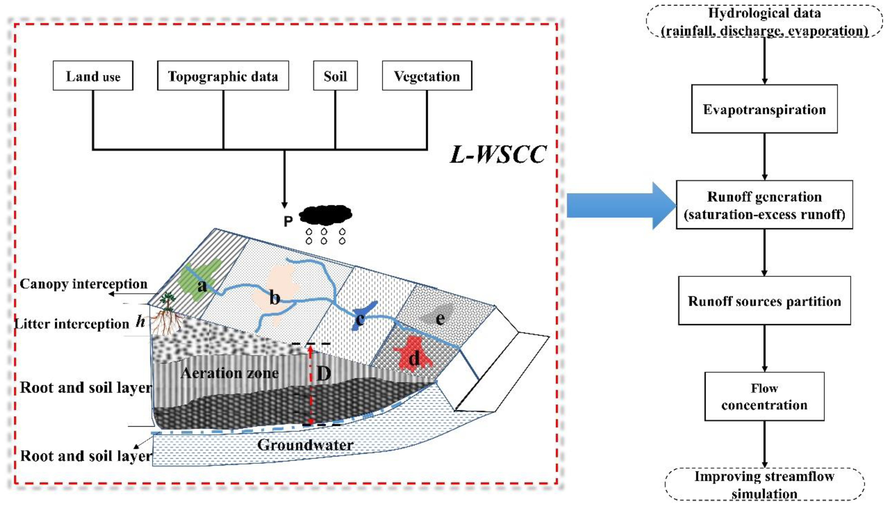
In this paper, the distribution of water storage capacity is calculated based on different land-use combined with relevant soil, terrain, vegetation, and other data, aiming to generate a WSCC with obvious physical meaning in entire watershed. On the basis of land-use and combined with the similarity of water storage capacity of different land-use types, the watershed is divided into five sub-regions: vegetation region (Figure 2a), bare land region (Figure 2b), reservoir region (Figure 2b), impervious surface region (hardened surface and buildings) (Figure 2d), and another region (Figure 2e).
Vegetation processes are often ignored in conceptual runoff [61]; however, for the watershed with good vegetation, the vegetation has a great influence on the runoff. Relevant studies have shown that the water storage capacity of vegetation mainly includes the canopy interception layer, the litter interception layer, and the water storage of soil and roots [24,27,62,63]. Therefore, the water storage capacity of the vegetation region is calculated as follows (more details in the Text S2 of Supplementary Material):
W i = f i × LAI i × h i + l i + N i × D i H i 100 ,
where W i is the storage capacity of the i-th grid located in the vegetation area (mm); f i   is the vegetation coverage of the i-th grid (0~1) ;   LAI i   is the vegetation leaf area index of the i-th grid; h i is the maximum water holding capacity of vegetation leaves in the i-th grid (mm); l i is litter interception (mm), obtained by remote sensing techniques or related research [64,65,66,67]; N i is non-capillary porosity (%), obtained by soil type; D i is thickness of aeration zone (mm), will be described later; H i is the depth of litter layer, generally is 50 mm. f i , LAI i , and h i can be determined by remote sensing data, and their physical meaning is clear.
For bare land, soil water storage capacity is the storage capacity between the field capacity and the wilting coefficient [14], which can be solved by soil and topographic index [68,69]:
W i = ( θ f , i θ w , i ) × D i ,
where W i is the tension water storage capacity of the i-th grid in bare land area, θ f , i is the field capacity (%), θ w , i is the wilting coefficient (%), D i is thickness of aeration zone (mm). θ f , i and θ w , i can be determined according to the soil type and can be obtained by soil water characteristics in soil-plant-atmosphere-water [70].
However, there is a difference between the WSCC and the real full storage state of the basin [24,71]. The modified calculation way of the water storage capacity in bare land area is as follows, which should be added:
W mod i = N i × D i 100 × 1 10 ,
where W mod i is the modified water storage capacity of the i-th grid in bare land area (mm).
For reservoir region and impervious surface region, if many small reservoirs or dams exist in the basin, the storage needs to be considered separately [72,73]. The hardened surface and other buildings have no or extremely small water storage capacity because the thickness of the aeration zone is 0 [74], so the water storage capacity is 0, W i = 0 .
Finally, for other regions, such as wetlands, lakes, and swamps, their water storage needs to be considered additionally if there are a large number of lakes, swamps, and wetlands in the basin. When calculating the water storage capacity of the basin, it can be adjusted according to the water storage data of swamps and lakes (interannual, monthly and seasonal). The change of wetland water storage capacity is small for a rainfall secondary flood, but its annual runoff changes greatly, which needs to be analyzed based on the wetland data over the years.
The thickness of aeration zone is critical for solving water storage capacity in Equations (1)–(3). At present, the thickness of aeration zone calculation is mostly based on the topographic index [68]:
D i = D ¯ S zm × [ TI i λ ] ,
where,   D i is the thickness of aeration zone on the i-th grid, T I i is the topographic index on the i-th grid, λ is the mean value of topographic index, D ¯ is the average saturated groundwater surface depth at the initial time, and S z m is the maximum storage depth in unsaturated area.
D ¯ and S z m have a relationship:
D ¯ = S zm Ln Q b Q 0 ,
Q b is the base flow at the outlet of the basin at the time of drought, Q 0 is the base flow at the outlet of the basin when the soil reaches saturation.   S z m can be obtained by base flow (digital filtering method) or the mass curve technique (MCT) [63,75,76].
Thickness of aeration zone can be obtained by Equation (4), whereas the thickness of impervious surface and water is 0, accordingly it needs to be adjusted by land-use. The scale problem of topographic index in Equation (4) has been discussed [77], and fitting method and multiscale method have been proposed [57,78,79]. A combination method is proposed to minimize the effect of scale. First, the multi-resolution method of topographic index is expressed as:
TIM i = 1 n j = 1 n Ln ( α j , i tan β j , i ) ,
M = 1 k i = 1 k TIM i   ,
where T I M i is the topographic index under multi-resolution;   α j , i is the single width catchment area of point i under the j-th scale, β j , i is the slope angle of point i under the j-th scale, λ M is the mean value of multi-resolution topographic index, n is the scale dimension, which is generally between 3 and 5 depending on the detail of data and watershed conditions, and k is the number of watershed grids.
Although the multi-resolution topographic index obtained above reduces the scale dependence to a certain extent, yet it depends on the parameter n . This paper selects a variety of fitting functions (Figure S4) and finally applied the generalized beta distribution of the second kind (best fits) to represent the watershed topographic index, which can be written as:
f ( TIM ) = r 3 bB ( r 1 , r 2 ) ( TIM b ) r 1 r 3 1 ( 1 + ( TIM b ) r 3 ) ( r 1 + r 2 ) ,
where, B ( r 1 , r 2 ) is Beta function, r 1 ,   r 2 , and r 3 are shape parameters and   r 1 > 0, r 2 > 0, r 3 > 0. The parameters r 1 and r 2 jointly determine the skewness of the distribution, and r 1 controls the shape of the left tail, r 2 controls the shape of the right tail, r 3 determines the global shape and affects the peak value of probability density function, b is the position parameter and its value depends on the TIM .

2.3. Data Preprocessing and Model Setting

According to the requirements of Equations (1)–(8), the data preprocessing for L-WSCC mainly includes the following steps: (1) Get the topographic index of the watershed; (2) obtain the thickness of aeration zone; (3) with soil parameters and vegetation parameters, the final distribution of water storage capacity under different land-use is calculated (Figure S5). Please see Text S3 for detailed processes.
To compare the performance of the WSCC and L-WSCC, two sets of simulations were implemented on hourly and daily scale. The PEST (parameter estimation) automatic calibration algorithm [80] was adopted for the calibration of the WSCC and other modules (evapotranspiration, runoff sources partition, and flow concentration) parameters based on Xinanjiang model. PEST is a model-independent nonlinear parameter estimation and uncertainty analysis program, which is a flexible and generic calibration tool [80]. It has the advantages of fast optimization speed and good robustness [81], which can be used in any of these hydrologic models and has been widely applied [82,83]. For the L-WSCC, the parameters were obtained by remote sensing data (mentioned in Section 2.3 and Section 2.4), the other modules parameter values were directly adopted from the calibrated WSCC. The parameters are listed in Table S3.

2.4. Evaluation Criteria

To evaluate the performance of WSCC and L-WSCC on daily scale, Nash–Sutcliffe efficiency (NSE), Kling–Gupta Efficiency (KGE), and percent bias error (BE) are calculated for the calibration (1982–1985) and validation (1986–1988) period. Daily NSE and BE values are compared with the values for basin-scale models recommended by related study, and model performance was classified as “very good”, “good”, “satisfactory”, and “unsatisfactory” [84] (Table S4). In addition, the appearance time of peak ( ARPT ) and flood peak error (PE) are also used to evaluate model performance on the hourly scale. In order to study the magnitude of impact of different factors on runoff yield, the change of mean absolute error (ΔMAE) is also used. Please see Text S4 for more details.

3. Results and Discussion

3.1. Results on Land-Use Change

In order to fully demonstrate the degree of land type transfer of Misai watershed from 1982 to 1988, the rate of land-use change is used to conduct the research [85] and the results are shown in Table 1. Due to the forest land and cultivated land accounting for about 95% of the watershed (Table S2), hence they play an essential role in hydrological processes, especially in runoff generation processes at Misai watershed. Therefore, we focus on changes in these two land-use types. Forest and cultivated land changed dramatically in 1986 (Figure S6 and Table 1), the rate of land-use change is 16.00% and −42.42%, respectively, which will have the greatest impact on the hydrological modelling (mentioned in Section 3.2, Section 3.3 and Section 3.4).

3.2. Calibration and Validation on Different Time-Scales

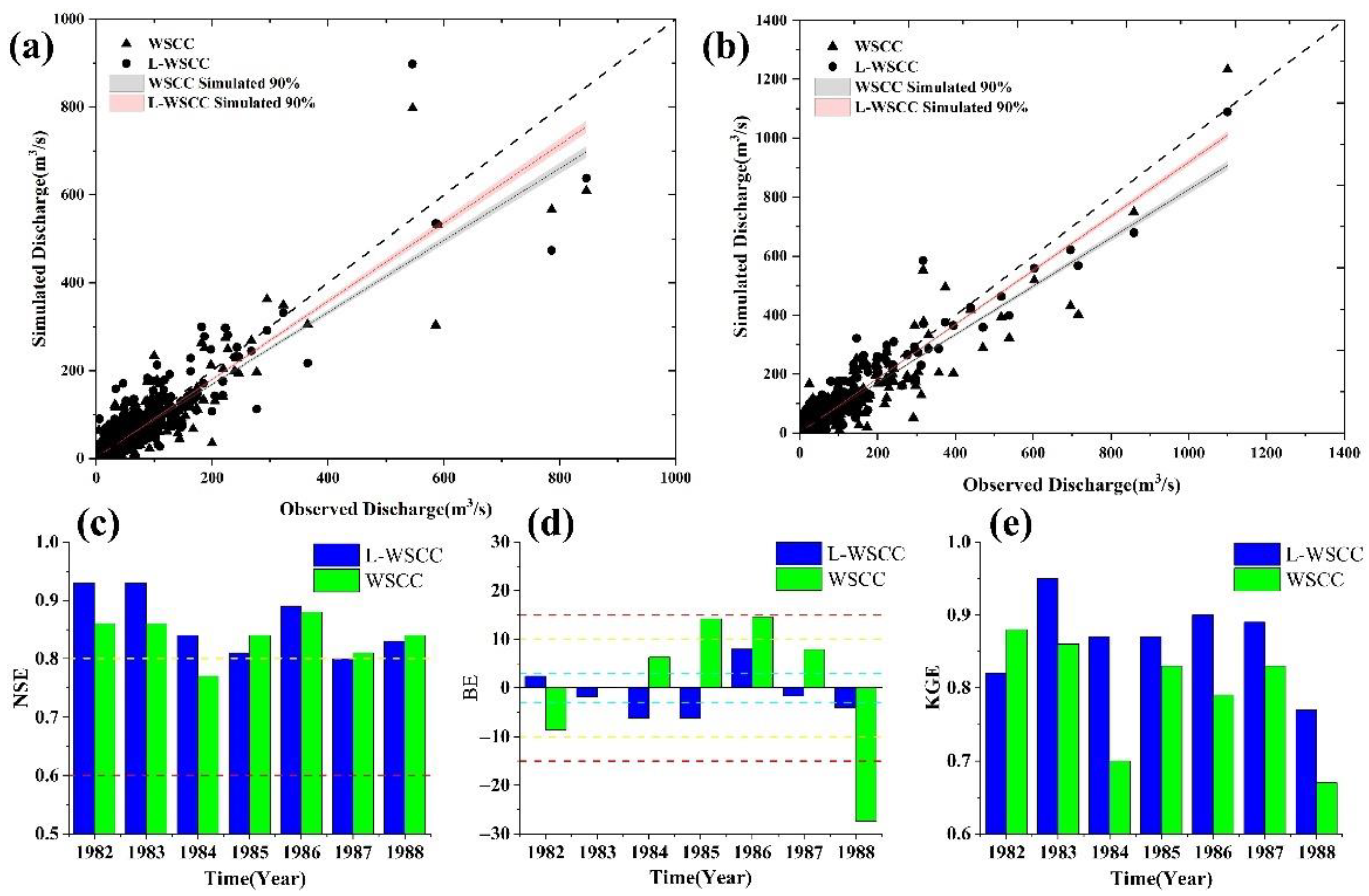
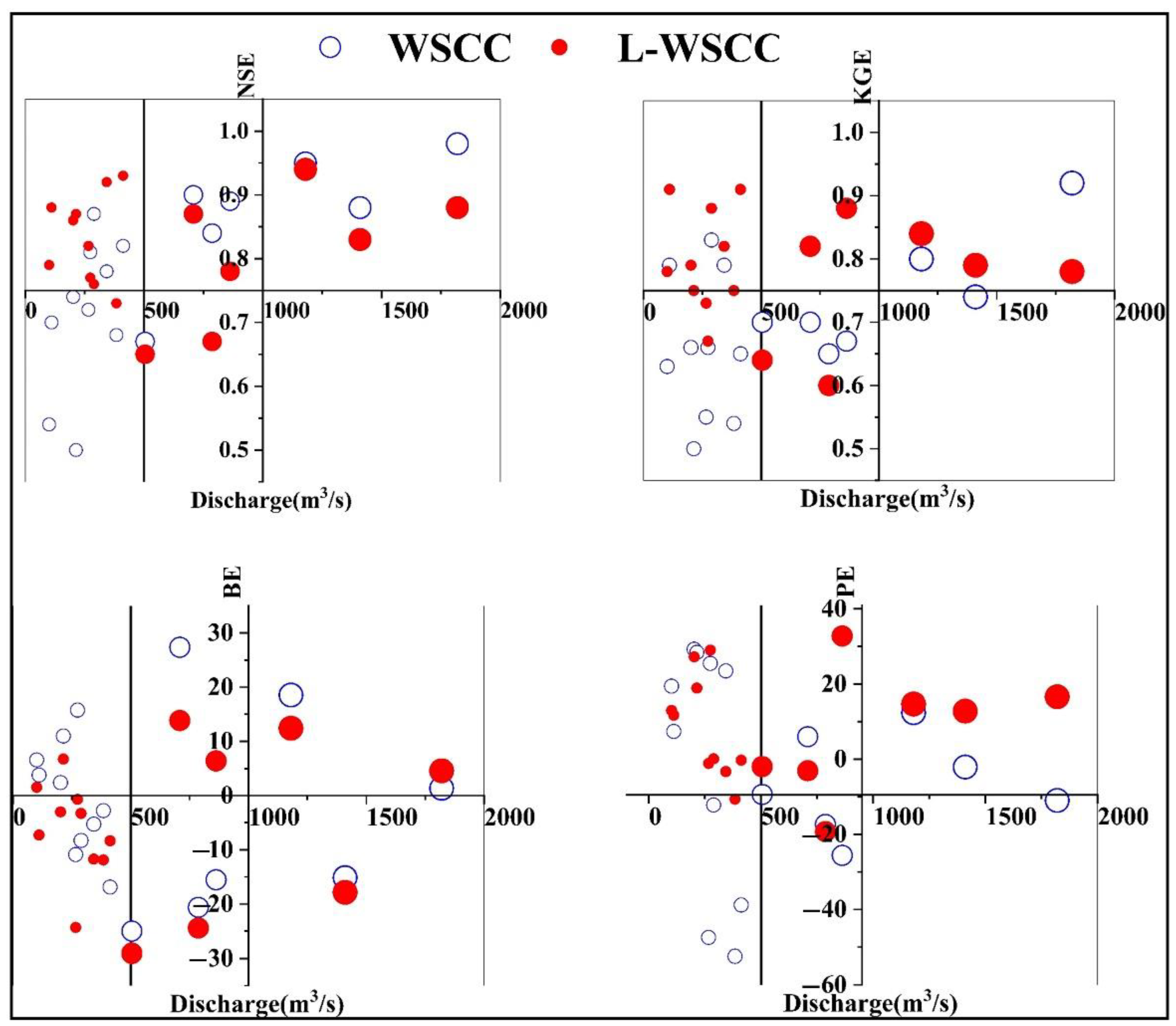
Comparing simulated and observed discharge at the outlet of the watershed, a close fit was observed with an R2 value above 0.7 whether calibration or verification period (Figure 3a,b). Additionally, the simulation effects of WSCC and L-WSCC can well meet the simulation requirements depending on the NSE and KGE (Figure 3c,e) and simulated streamflow hydrographs matched the observed data well (Figure S7). No significant model over or underestimation was found, since the obtained parameter values are in the recommended range. Nevertheless, compared with WSCC, L-WSCC significantly improved the flood volumes: L-WSCC improved the BE by 3.10% and 12.02% during calibration and validation period, respectively (Table S5). Even worse, there was a sudden change in the simulation performance of WSCC in terms of BE in validation period (Figure 3d), especially, WSCC gets “unsatisfactory” result in 1988, which may be due to the fact that WSCC uses the initial calibration parameters whereas the land-use has changed strongly at this time (Table 1). However, the L-WSCC performs equally well indicating that integrated approach considers the impact of land-use on runoff yield, so it is more flexible (than WSCC) to handle differences in the rainfall and runoff in validation period. This corresponds to the purpose of our research.
In addition to the daily scale, 17 representative floods from 1982 to 1988 are chosen to evaluate the simulation performance of L-WSCC on rainstorm process (hourly scale).
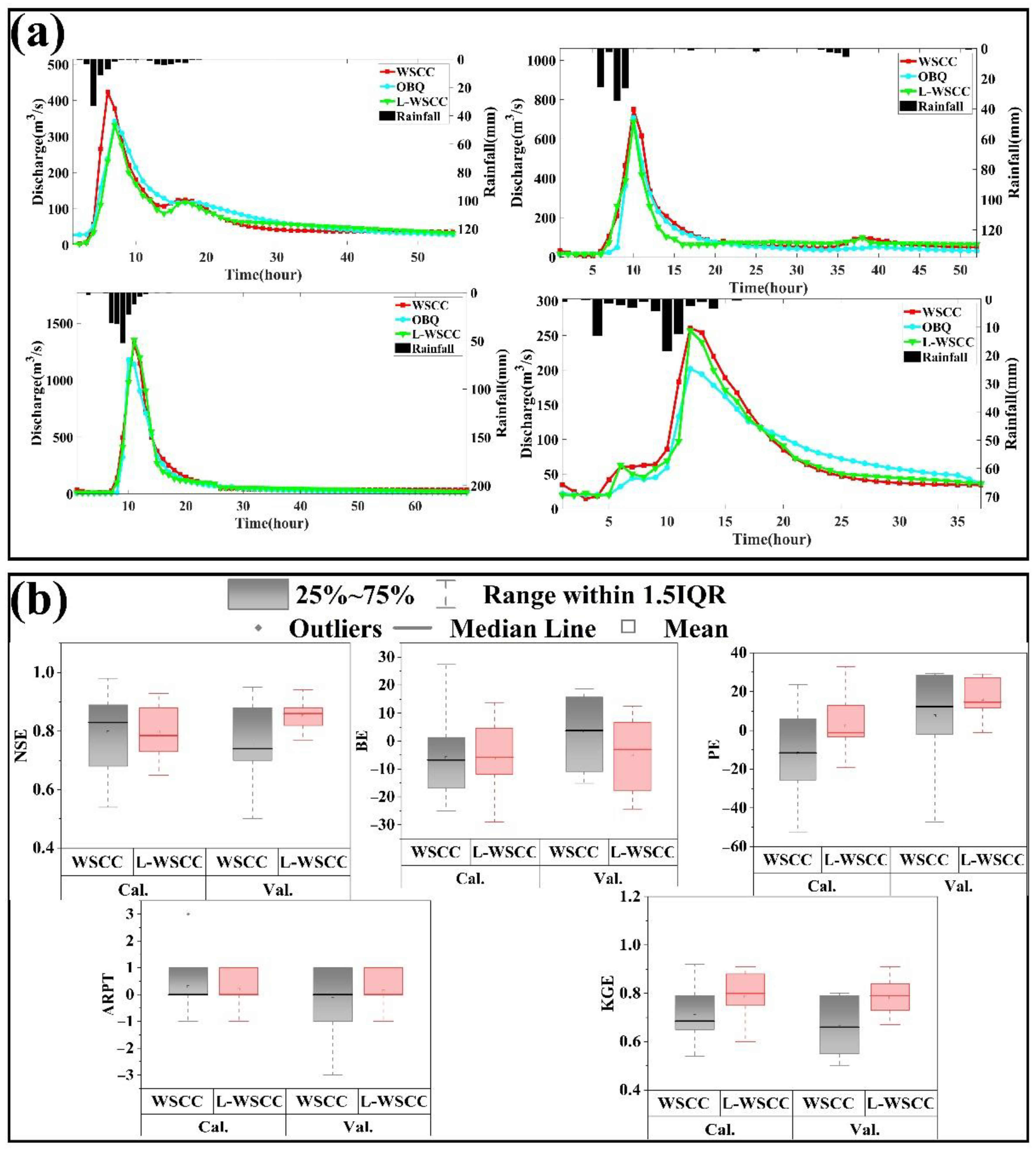
The hydrographs of these floods are shown in Figure S8 and Figure 4a. The performance statistics are shown in Figure 4b. WSCC and L-WSCC resulted in at least satisfactory performance (NSE > 0.5) during the calibration and validation period (Figure 4b). The mean value of NSE were 0.78 and 0.82 of WSCC and L-WSCC considering the entire period, indicating that the WSCC and L-WSCC can reasonably predict the general shapes of the storm hydrographs in Misai watershed.
L-WSCC achieves better results compared to WSCC on the hourly scale with the NSE of L-WSCC increased from 0.76 to 0.85 during the validation period, PE decreased from values of approximately 21.56% to 10.10% and from 21.79% to 16.50% during the calibration and validation period, respectively (Table S6 and Figure 4b). When the BE is less than 20%, we think it is qualified. The BE qualified rate of WSCC is 70% in calibration period, and all qualified in the validation period, 80% and 86% in L-WSCC, respectively. The BE decreased from approximately 12.96% to 11.50% compared to WSCC during the calibration period and from 11.07% to 10.33% during the validation period (Figure 4b).
Despite the good performance in reproducing flood volumes, the PE was unsatisfactory (PE > 20%) for some floods (40.00% of the floods during the calibration period and 57.14% during the validation period of WSCC, while only 10.00% of the floods during the calibration period and 28.57% during the validation period of L-WSCC). This result indicated that WSCC has markedly poorer performance for the validation period, which experiences higher variability in runoff than the calibration period, suggesting that WSCC cannot be accepted in the validation period. Hence, the parameters of WSCC and L-WSCC calibrated were able to reproduce runoff generation process but failed to capture the behavior of confluence process at the basin scale. These bad simulations occurred after 1985 (64% in all bad events). This is because of the fact that the land-use in the watershed has changed dramatically in 1986 and affected the confluence of the watershed, resulting in the unreliable simulation results.
Figure 4a demonstrates the visual contrast of observed and simulated discharge time series to investigate the similarity of discharge in the watershed. The overall shape of the discharge hydrograph matches well with the observed discharge. However, the peak discharge is degraded during both runs. This degradation is mainly due to frequent negative updates (reduction) in the surface runoff, which is more affected by land-use change while L-WSCC weakens the impact of land-use on it. Hence, the simulated runoff series from the L-WSCC corresponds fairly well with the observed data (compared with WSCC), even though minor discrepancies still exist for the peak discharge simulation.

3.3. Seasonal Variation of Simulation

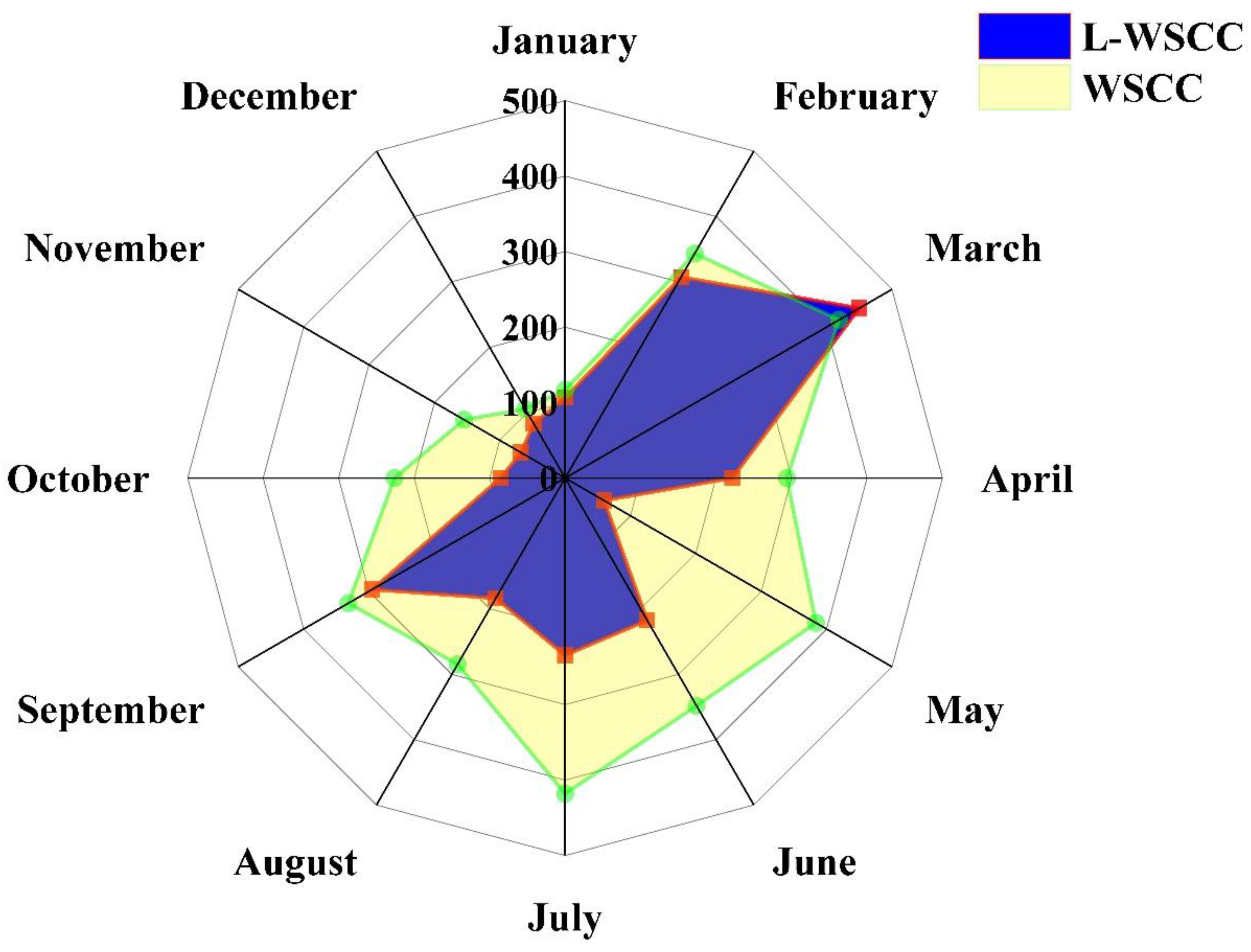
The observed and simulated discharge of every month have been analyzed and the mean absolute error (MAE) are shown in Figure 5. L-WSCC runoff simulation results are better than WSCC in the rainy season (May–July). The main reasons are: most of the remote sensing data used are from around June (Section 2.1). The water storage capacity calculation for runoff generation from May to July is more accurate. For other months, such as from September to April, the vegetation growth status is less than that in rainy season, which will influence the simulation results of L-WSCC. Therefore, the improvement effect of L-WSCC during this period is not as obvious as that in the rainy season (Figure 5). For WSCC, the runoff simulation results are better for the rainy season because WSCC is suitable for the simulation of large floods. Therefore, how to improve the simulation effect in dry season needs further research.

3.4. Simulation in Different Flood Types

To understand the simulation performance of WSCC and L-WSCC in different flood types, 21 floods are divided into three typical flood processes: big (B: peak discharge > 1000 m3/s), medium (M: 500 m3/s < peak discharge ≤ 1000 m3/s), and small (S: peak discharge ≤ 500 m3/s) floods according to the observed peak discharge. The simulated and observed values of WSCC and L-WSCC are shown in Figure S9. The discharges relationship in big floods is very good, but not so good in small and medium floods, especially small floods. This is noteworthy as the initial soil deficit has a greater impact on small floods and this is also consistent with the phenomenon that small floods are more easily disturbed by human activities. The NSE/KGE of the L-WSCC is greatly improved compared with the WSCC in small and medium floods, especially for small floods (Table S7 and Figure 6). However, there is very little difference between the WSCC and L-WSCC for big floods (Figure 6). This is expected because the watershed is close to saturation-excess state, and all rainfall produces runoff yield in big floods. Although there is a certain improvement in terms of BE, the flood volume of some events is obviously less (lower 20%), which may be caused by artificial interception. In summary, L-WSCC has a significant improvement of small and medium floods, but almost no improvement for large floods. This corresponds to the impact of land-use on saturation-excess runoff.

3.5. The Local Sensitivity Analysis of Different Driving Factors

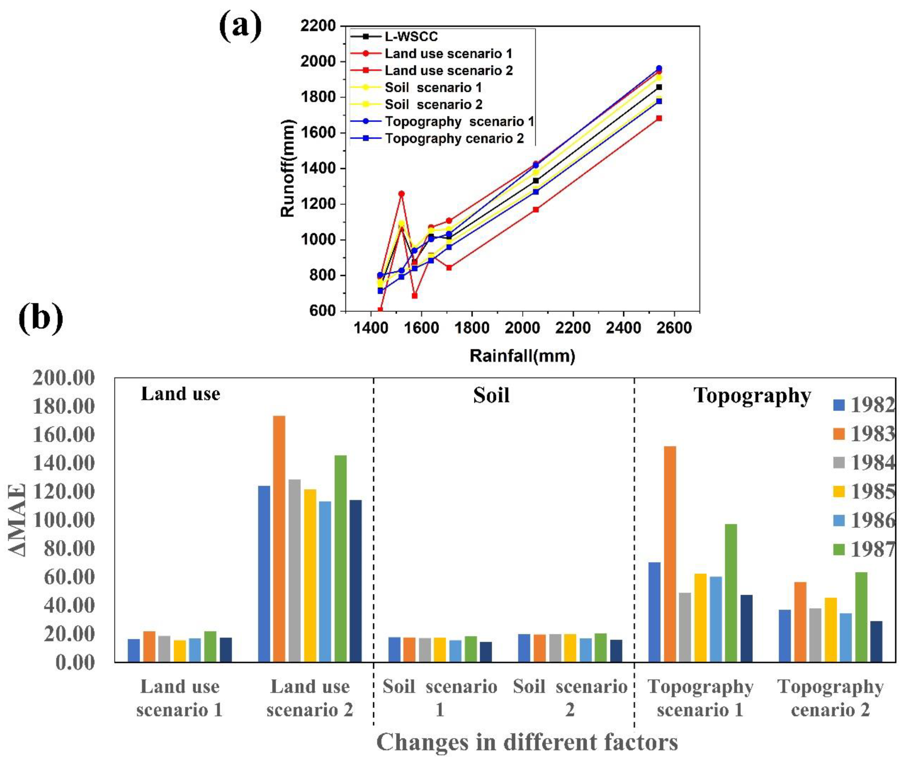
To investigate the magnitude of impact of different factors on runoff yield, the sensitivity of model input parameters was evaluated through local sensitivity analysis by adjusting different factor parameters by ±10% to construct different scenarios: (a) land-use scenarios. The area of bare land and vegetation is increased by 10% (according to Section 2.3), and the scenarios are land-use scenario 1 and land-use scenario 2, respectively. (b) Soil scenarios. The soil parameters are increased and decreased by 10%, and the scenarios are soil scenario 1 and soil scenario 2 respectively. (c) Topography scenarios. The topography parameters are increased and decreased by 10%, and the scenarios are topography scenario 1 and topography scenario 2 respectively. Figure 7a shows the relationship between rainfall and runoff under different scenarios. An upward or downward shift in the relationship indicated that the relationship between rainfall and runoff has been altered by land-use, soil, and topography, correspondingly. However, the original relationship between rainfall and runoff is the same. As the parameter changes, the rainfall-runoff relationship changes in different directions (Figure 7a). Remarkably, the bare land (land-use scenario 1) has an enhancing effect on the runoff, while the vegetation (land-use scenario 2) has a significant inhibitory effect. Similarly, changes of soil parameters and topography parameters also cause changes in different trends of runoff (above and below the L-WSCC line, respectively). In addition, it should be noted that the degrees of influence for different factors on the runoff are different; land-use has the greatest, followed by topography, with the lowest for soil. Moreover, vegetation changes have the deepest impact on runoff (the farthest distance to the line of the L-WSCC). Moreover, the higher the rainfall, the greater the increase in the runoff difference, suggesting that the relationship between rainfall and runoff is more sensitive to different factors with increasing rainfall. Figure 7b shows the changes of MAE in different scenarios and we can also find that different land-use has a great influence on the runoff yield. When the bare land region is changed, the ΔMAE is about 20%, but when the vegetation region is changed, the ΔMAE changes to 113.97–173.14% with the average is 131.38%. For the soil scenarios, the ΔMAE is relatively small (about 20%), indicating that the runoff yield is less sensitive to soil factors. For the topography scenarios, although ΔMAE has changed, the variation range is between the land-use and soil factors (about 60%), demonstrating that the sensitivity of topography factors is between the land-use and soil factors. These results suggest that the land-use is the largest of the explanatory variable, revealing that land-use is the most significant driver for runoff yield.

3.6. Strength and Recommendations for Future Studies

This study systematically evaluated the integrated approach proposed by remote sensing and WSCC in the Misai watershed. Compared to WSCC, L-WSCC obtained more satisfactory results (Section 3.2, Section 3.3 and Section 3.4), revealing its potential in hydrological modeling considering human activities at watershed scale. These results were related to the difference in the runoff generation structure of the WSCC and L-WSCC, in which L-WSCC considered the underlying surface change on runoff yield. The results of local sensitivity analysis (Section 3.5) suggested that land-use plays an important role in runoff yield and is consistent with our study. The information and knowledge obtained from remote sensing data and WSCC were coupled together, facilitated addressing the problem and predicting the runoff yield, and provided a calculation method in ungauged basins [86,87]. In addition, runoff generation parameters of L-WSCC were obtained from remote sensing data without calibration, thus, L-WSCC can eliminate a source of parameter uncertainties. Taking this approach further, it is also applicable to the runoff generation part of other rainfall-runoff models based on saturation-excess runoff such as VIC [88], GR4 J [89], PDM [90], ARNO [91], HBV [92], G2G [54], unifying the distribution of WSCC for all these models.
Although study objectives generally are achieved, this study has limitations that should be outlined and perhaps targeted in forthcoming studies. First, the influence of climatic factors on runoff yield is not considered in L-WSCC. Despite this will not have an impact on the results of this study, it cannot be ignored if long-term runoff predictions are carried [93]. Second, although multi-resolution and fitting method are used to minimize the effect of topography scale, the accuracy of land-use, soil, vegetation, and other data has not been considered. The solution of the problem will have maximized the accuracy of our model. Furthermore, seasonal variation of simulation results indicates that the acquisition time of remote sensing data has a certain influence on the simulation results. Higher temporal resolution data for the improvement of simulation needs further study. Moreover, the study period is quite long ago and the basin hydrology may be substantially altered. Therefore, obtaining more recent data for comparative research is the direction of our further research. Although this study has obtained good results in the short-term hydrological simulation (1982–1988), the long-term hydrological process of the basin will inevitably be affected by climate change, so it is worth exploring how to take the climate factors into account for the long-term hydrological simulation. Notwithstanding these limitations, this study outlines a comprehensive runoff generation process for flood simulation based on remote sense and WSCC. L-WSCC considers the impact of human activities on runoff yield, enhances the physical meaning of WSCC, and can better understand the hydrological process. Extreme floods events are expected to occur more frequently, and the integrated approach will help relevant departments implement corresponding measures.

4. Conclusions

A new integrated approach (L-WSCC) combined the various remote sensing factors and saturation-excess runoff was proposed at basin scale, which helped to clarify the difference between the distribution of water storage capacity in reality and the modelled runoff. Unlike the traditional WSCC method, the extended L-WSCC consisted of equations of the effect of different factors on runoff, which provided beneficial insights in understanding the behaviors of the rainfall-runoff process. L-WSCC enhanced the physical meaning of the original WSCC, and simulating flood in regions characterized by physical basis rather than calibration/empirical approach. L-WSCC was evaluated from the Misai basin to be very effective in flood simulation and the results showed that the physics-based approach is promising. The major findings of this paper are summarized as follows:
(1)
The application of L-WSCC in Misai basin demonstrated that the method proposed in this article performed well in hydrological simulating at the different timescales (mean NSE: 0.86 for daily scale, 0.82 for hourly scale; mean BE: 4.34% for daily scale, 11.02% for hourly scale). The results have proven to be robust and reliable, which were powerful evidence for the reasonability of the construction process of L-WSCC.
(2)
The contrasting results confirmed that L-WSCC performed favorably compared to the empirical WSCC method and identified novel L-WSCC with high confidence in flood simulation (mean NSE increased from 0.78 to 0.82, mean PE decreased from 21.66% to 12.74%, mean RE decreased from 12.18% to 11.02%). These results indicated that the L-WSCC can derive a set of feasible values for the runoff generation.
(3)
The correction of hydrologic responses resulting from L-WSCC is more obvious for relatively small flood event (increased by 15.96% of small floods in terms of mean NSE). The proposed method can more accurately capture the runoff process of small flood events according to various remote sensing factors, thereby improving the ability of WSCC to simulate small floods. Thus, the newly proposed model may better represent runoff generation that previously have been beyond the scope of the traditional WSCC method (which is considered to work well for large flood events simulation).
(4)
The results of sensitivity analysis showed that land-use and land cover (especially the change of vegetation) have the greatest impact on yield (mean ΔMAE: 131.38%), which demonstrated that land-use have a predominant control on runoff yield in the short term.
The benefit of the spatially distributed method (L-WSCC) indeed mainly lies in the broader range of applications such as spatial scenario simulations and the ability to runoff simulation in similar basins. Our suggested approach can serve as an alternative to regionalization techniques, when one is interested in runoff simulation at ungauged internal stations of a particular scale. Moreover, this new spatial description of runoff provided by L-WSCC may allow for a more realistic extension of the WSCC method to runoff related processes such as water quality model and sediment migration model.

Supplementary Materials

The following supporting information can be downloaded at: https://www.mdpi.com/article/10.3390/w14182854/s1, Figure S1. Topographic information of the study area. Figure S2. Land use of study area. Figure S3. The soil and vegetation of the study area. (a) Soil types (b) vegetation types. Figure S4. Different fitting functions of the probability density of topographic index. Figure S5. Spatial distribution of water storage capacity under different land use (The water storage capacity of Water and Urban land is 0, not shown). Figure S6. Land use land cover dynamics in Misai basin. Figure S7. The observed and simulated streamflow hydrographs (daily scale) during: a: calibration and b: validation period. Figure S8. Comparison between observed and simulated discharge hydrographs (hourly scale) during: a: calibration and b: validation period. Figure S9. Simulated and observed discharge under different flood types (all calibration and validation period) (a: big floods, b: medium floods, c: small floods). Figure S10. (a) The water storage capacity curve; (b) Rainfall-runoff relationship. Figure S11. Topographic index distribution under four different scales in Misai basin (30 m,100 m,200 m,500 m). Figure S12. Topographic index frequency distribution histogram under four different scales in the Misai basin (30 m,100 m,200 m,500 m). Figure S13. Probability density of topographic index at different scales. Figure S14. Probability density of topographic index (the sum of the 4 scales). Figure S15. The final topographic index after pre-treatments. Figure S16. Aeration zone of Misai basin (a: before land use correction; b: after land use correction). Figure S17. a: Field capacity; b: Wilting coefficient; c: Full storage coefficient. Figure S18. Vegetation information of Misai basin. Figure S19. Canopy interception of vegetation in Misai basin. Figure S20. Spatial dis-tribution of water storage capacity in vegetation region. Figure S21. Water storage capacity curve under different land use in vegetation region. Table S1. The 17 typical flood processes (1982–1988). Table S2. The land use information. Table S3. The parameters of WSCC. Table S4. Grade table of model performance. Table S5. The model performance on daily scale (V, G, S and US represent very good, good, satisfactory and unsatisfactory respectively). Table S6. The model performance on hourly scale. Table S7. The evaluation results under different types of floods (all calibration and validation period). Text S1. the description of WSCC. Text S2. The Water Storage Capacity Cal-culation in Vegetation region. Text S3. Data. Text S4. Statistical Criteria and Model Evaluation Performance.

Author Contributions

Conceptualization, C.X. and J.Y.; methodology, C.X. and H.F.; software, C.X.; validation, C.X., J.Y. and C.G.; formal analysis, C.X. and H.F.; investigation, H.F.; resources, H.F.; data curation, C.X. and H.F.; writing—original draft preparation, C.X. and H.F.; writing—review and editing, J.Y. and C.G.; visualization, J.Y. and H.F.; supervision, H.F.; project administration, C.X. and H.F.; funding acquisition, C.X. All authors have read and agreed to the published version of the manuscript.

Funding

This research was funded by the Major Science and Technology Program for Water Pollution Control and Treatment, grant number 2014ZX07203-008.

Institutional Review Board Statement

Not applicable.

Informed Consent Statement

Not applicable.

Data Availability Statement

The data that support the findings of this study are available from the corresponding author upon reasonable request.

Acknowledgments

The authors would like to acknowledge Xiaoliu Yang of Peking University, China for his theoretical support and guidance.

Conflicts of Interest

The authors declare no conflict of interest.

References

  1. Wang, Y.T.; Chen, A.S.; Fu, G.T.; Djordjevic, S.; Zhang, C.; Savic, D.A. An integrated framework for high-resolution urban flood modelling considering multiple information sources and urban features. Environ. Modell. Softw. 2018, 107, 85–95. [Google Scholar] [CrossRef]
  2. Dou, Y.H.; Ye, L.; Gupta, H.V.; Zhang, H.R.; Behrangi, A.; Zhou, H.C. Improved Flood Forecasting in Basins with No Precipitation Stations: Constrained Runoff Correction Using Multiple Satellite Precipitation Products. Water Resour. Res. 2021, 57, 29682. [Google Scholar] [CrossRef]
  3. Toosi, A.S.; Calbimonte, G.H.; Nouri, H.; Alaghmand, S. River basin-scale flood hazard assessment using a modified multi-criteria decision analysis approach: A case study. J. Hydrol. 2019, 574, 660–671. [Google Scholar] [CrossRef]
  4. Sugianto, S.; Deli, A.; Miswar, E.; Rusdi, M.; Irham, M. The Effect of Land Use and Land Cover Changes on Flood Occurrence in Teunom Watershed, Aceh Jaya. Land 2022, 11, 1271. [Google Scholar] [CrossRef]
  5. Li, X.G. A new method to evaluate floodwater for control/use in high-sediment rivers of Northwest China. Sci. Rep. 2017, 7, 17219. [Google Scholar] [CrossRef]
  6. Archer, D.R.; Fowler, H.J. Characterising flash flood response to intense rainfall and impacts using historical information and gauged data in Britain. J. Flood Risk Manag. 2018, 11, S121–S133. [Google Scholar] [CrossRef]
  7. Zhou, Q.Q.; Leng, G.Y.; Feng, L.Y. Predictability of state-level flood damage in the conterminous United States: The role of hazard, exposure and vulnerability. Sci. Rep. 2017, 7, 5334. [Google Scholar] [CrossRef]
  8. Breinl, K.; Lun, D.; Muller-Thomy, H.; Bloschl, G. Understanding the relationship between rainfall and flood probabilities through combined intensity-duration-frequency analysis. J. Hydrol. 2021, 602, 126759. [Google Scholar] [CrossRef]
  9. Liu, W.M.; Carling, P.A.; Hu, K.H.; Wang, H.; Zhou, Z.; Zhou, L.Q.; Liu, D.Z.; Lai, Z.P.; Zhang, X.B. Outburst floods in China: A review. Earth Sci. Rev. 2019, 197, 102859. [Google Scholar] [CrossRef]
  10. Zhang, W.Y. Application of NRCS-CN method for estimation of watershed runoff and disaster risk. Geomat. Nat. Hazards Risk 2019, 10, 2220–2238. [Google Scholar] [CrossRef] [Green Version]
  11. Oladotun, O.M. Assessment of Runoff Potential for Disaster Risk Reduction Using Geospatial Technology in Opa Watershed, Southwestern Nigeria. S. Afr. J. Geomat. 2021, 10, 90–100. [Google Scholar] [CrossRef]
  12. Guan, M.F.; Sillanpaa, N.; Koivusalo, H. Storm runoff response to rainfall pattern, magnitude and urbanization in a developing urban catchment. Hydrol. Process 2016, 30, 543–557. [Google Scholar] [CrossRef]
  13. Erena, S.H.; Worku, H. Dynamics of land use land cover and resulting surface runoff management for environmental flood hazard mitigation: The case of Dire Daw city, Ethiopia. J. Hydrol. Reg. Stud. 2019, 22, 100598. [Google Scholar] [CrossRef]
  14. Zhao, R.J. The Xinanjiang Model Applied in China. J. Hydrol. 1992, 135, 371–381. [Google Scholar] [CrossRef]
  15. Alazzy, A.A.; Lu, H.S.; Zhu, Y.H. Assessing the Uncertainty of the Xinanjiang Rainfall-Runoff Model: Effect of the Likelihood Function Choice on the GLUE Method. J. Hydrol. Eng. 2015, 20, 1943–5584. [Google Scholar] [CrossRef]
  16. Gong, J.F.; Yao, C.; Li, Z.J.; Chen, Y.F.; Huang, Y.C.; Tong, B.X. Improving the flood forecasting capability of the Xinanjiang model for small- and medium-sized ungauged catchments in South China. Nat. Hazards 2021, 106, 2077–2109. [Google Scholar] [CrossRef]
  17. Liao, S.L.; Li, G.; Sun, Q.Y.; Li, Z.F. Real-time correction of antecedent precipitation for the Xinanjiang model using the genetic algorithm. J. Hydroinform. 2016, 18, 803–815. [Google Scholar] [CrossRef]
  18. Yao, C.; Zhang, K.; Yu, Z.B.; Li, Z.J.; Li, Q.L. Improving the flood prediction capability of the Xinanjiang model in ungauged nested catchments by coupling it with the geomorphologic instantaneous unit hydrograph. J. Hydrol. 2014, 517, 1035–1048. [Google Scholar] [CrossRef]
  19. Gao, H.K.; Cai, H.Y.; Duan, Z. Understanding the impacts of catchment characteristics on the shape of the storage capacity curve and its influence on flood flows. Hydrol. Res. 2018, 49, 90–106. [Google Scholar] [CrossRef]
  20. Tran, Q.Q.; De Niel, J.; Willems, P. Spatially Distributed Conceptual Hydrological Model Building: A Genetic top-Down Approach Starting From Lumped Models. Water Resour. Res. 2018, 54, 8064–8085. [Google Scholar] [CrossRef] [Green Version]
  21. Badjana, H.M.; Fink, M.; Helmschrot, J.; Diekkruger, B.; Kralisch, S.; Afouda, A.A.; Wala, K. Hydrological system analysis and modelling of the Kara River basin (West Africa) using a lumped metric conceptual model. Hydrolog. Sci. J. 2017, 62, 1094–1113. [Google Scholar] [CrossRef]
  22. Chen, X.; Chen, Y.D.; Xu, C.Y. A distributed monthly hydrological model for integrating spatial variations of basin topography and rainfall. Hydrol. Process. 2007, 21, 242–252. [Google Scholar] [CrossRef]
  23. Jayawardena, A.W.; Zhou, M.C. A modified spatial soil moisture storage capacity distribution curve for the Xinanjiang model. J. Hydrol. 2000, 227, 93–113. [Google Scholar] [CrossRef]
  24. Zhuo, L.; Han, D.W. Misrepresentation and amendment of soil moisture in conceptual hydrological modelling. J. Hydrol. 2016, 535, 637–651. [Google Scholar] [CrossRef]
  25. Bartlett, M.S.; Parolari, A.J.; McDonnell, J.J.; Porporato, A. Beyond the SCS-CN method: A theoretical framework for spatially lumped rainfall-runoff response. Water Resour. Res. 2016, 52, 4608–4627. [Google Scholar] [CrossRef]
  26. Bartlett, M.S.; Daly, E.; McDonnell, J.J.; Parolari, A.J.; Porporato, A. Stochastic rainfall-runoff model with explicit soil moisture dynamics. Proc. R. Soc. A Math. Phys. Eng. Sci. 2015, 471, 20150389. [Google Scholar] [CrossRef]
  27. Shi, P.F.; Yang, T.; Xu, C.Y.; Yong, B.; Huang, C.S.; Li, Z.Y.; Qin, Y.W.; Wang, X.Y.; Zhou, X.D.; Li, S. Rainfall-Runoff Processes and Modelling in Regions Characterized by Deficiency in Soil Water Storage. Water 2019, 11, 1858. [Google Scholar] [CrossRef]
  28. Guo, W.J.; Wang, C.H.; Zeng, X.M.; Ma, T.F.; Yang, H. Subgrid Parameterization of the Soil Moisture Storage Capacity for a Distributed Rainfall-Runoff Model. Water 2015, 7, 2691–2706. [Google Scholar] [CrossRef]
  29. Sivapalan, M.; Woods, R.A. Evaluation of the Effects of General-Circulation Models Subgrid Variability and Patchiness of Rainfall and Soil-Moisture on Land-Surface Water-Balance Fluxes. Hydrol. Process. 1995, 9, 697–717. [Google Scholar] [CrossRef]
  30. Yao, C.; Li, Z.J.; Bao, H.J.; Yu, Z.B. Application of a Developed Grid-Xinanjiang Model to Chinese Watersheds for Flood Forecasting Purpose. J. Hydrol. Eng. 2009, 14, 923–934. [Google Scholar] [CrossRef]
  31. Meng, C.Q.; Zhou, J.Z.; Zhong, D.Y.; Wang, C.; Guo, J. An Improved Grid-Xinanjiang Model and Its Application in the Jinshajiang Basin, China. Water 2018, 10, 1265. [Google Scholar] [CrossRef]
  32. Yao, C.; Li, Z.J.; Yu, Z.B.; Zhang, K. A priori parameter estimates for a distributed, grid-based Xinanjiang model using geographically based information. J. Hydrol. 2012, 468, 47–62. [Google Scholar] [CrossRef]
  33. Fowler, K.J.A.; Peel, M.C.; Western, A.W.; Zhang, L.; Peterson, T.J. Simulating runoff under changing climatic conditions: Revisiting an apparent deficiency of conceptual rainfall-runoff models. Water Resour. Res. 2016, 52, 1820–1846. [Google Scholar] [CrossRef]
  34. Beven, K.; Freer, J. A dynamic TOPMODEL. Hydrol. Process. 2001, 15, 1993–2011. [Google Scholar] [CrossRef]
  35. Chang, B.X.; Wherley, B.; Aitkenhead-Peterson, J.A.; McInnes, K.J. Effects of urban residential landscape composition on surface runoff generation. Sci. Total Environ. 2021, 783, 146977. [Google Scholar] [CrossRef]
  36. Ren, L.L.; Wang, G.Z.; Fang, L.U. Application of spatially varying storage capacity model for runoff parameterization in semi-arid catchment. Water Sci. Eng. 2009, 2, 1–10. [Google Scholar] [CrossRef]
  37. Yuan, F.; Ren, L. Application of the Xinanjiang vegetation-hydrology model to streamflow simulation over the Hanjiang River basin, China. Hydrol. Mt. Reg. Obs. Process. Dyn. 2009, 82, 2273–2278. [Google Scholar] [CrossRef]
  38. Feng, X.M.; Sun, G.; Fu, B.J.; Su, C.H.; Liu, Y.; Lamparski, H. Regional effects of vegetation restoration on water yield across the Loess Plateau, China. Hydrol. Earth Syst. Sci. 2012, 16, 2617–2628. [Google Scholar] [CrossRef]
  39. Cerda, A.; Lucas-Borja, M.E.; Franch-Pardo, I.; Ubeda, X.; Novara, A.; Lopez-Vicente, M.; Popovic, Z.; Pulido, M. The role of plant species on runoff and soil erosion in a Mediterranean shrubland. Sci. Total Environ. 2021, 799, 149218. [Google Scholar] [CrossRef]
  40. Crosson, W.L.; Limaye, A.S.; Laymon, C.A. Parameter sensitivity of soil moisture retrievals from airborne C- and X-band radiometer measurements in SMEX02. IEEE Trans. Geosci. Remote Sens. 2005, 43, 2842–2853. [Google Scholar] [CrossRef]
  41. Crave, A.; GascuelOdoux, C. The influence of topography on time and space distribution of soil surface water content. Hydrol. Process. 1997, 11, 203–210. [Google Scholar] [CrossRef]
  42. Western, A.W.; Grayson, R.B.; Bloschl, G.; Willgoose, G.R.; McMahon, T.A. Observed spatial organization of soil moisture and its relation to terrain indices. Water Resour. Res. 1999, 35, 797–810. [Google Scholar] [CrossRef]
  43. Wilson, D.J.; Western, A.W.; Grayson, R.B. A terrain and data-based method for generating the spatial distribution of soil moisture. Adv. Water Resour. 2005, 28, 43–54. [Google Scholar] [CrossRef]
  44. Zhao, Q.; Gong, H.L.; Deng, W.; Wang, S.Y.; Zhao, W.J.; An, X.S.; Gong, Z.N.; Zhang, Z.Q. Using DEM to quantify spatial variability of soil storage capacity: A semi-distribtited hydrological model for northern China. Int. Geosci. Remote Sens. Symp. 2005, 6, 4429–4432. [Google Scholar]
  45. Sivapalan, M.; Woods, R.A.; Kalma, J.D. Variable bucket representation of TOPMODEL and investigation of the effects of rainfall heterogeneity. Hydrol. Process. 1997, 11, 1307–1330. [Google Scholar] [CrossRef]
  46. Gao, H.K.; Birkel, C.; Hrachowitz, M.; Tetzlaff, D.; Soulsby, C.; Savenije, H.H.G. A simple topography-driven and calibration-free runoff generation module. Hydrol. Earth Syst. Sci. 2019, 23, 787–809. [Google Scholar] [CrossRef]
  47. Mu, W.B.; Yu, F.L.; Li, C.Z.; Xie, Y.B.; Tian, J.Y.; Liu, J.; Zhao, N.N. Effects of Rainfall Intensity and Slope Gradient on Runoff and Soil Moisture Content on Different Growing Stages of Spring Maize. Water 2015, 7, 2990–3008. [Google Scholar] [CrossRef]
  48. Defersha, M.B.; Melesse, A.M. Effect of rainfall intensity, slope and antecedent moisture content on sediment concentration and sediment enrichment ratio. Catena 2012, 90, 47–52. [Google Scholar] [CrossRef]
  49. Schneiderman, E.M.; Steenhuis, T.S.; Thongs, D.J.; Easton, Z.M.; Zion, M.S.; Neal, A.L.; Mendoza, G.F.; Walter, M.T. Incorporating variable source area hydrology into a curve-number-based watershed model. Hydrol. Process. 2007, 21, 3420–3430. [Google Scholar] [CrossRef]
  50. Penna, D.; Tromp-van Meerveld, H.J.; Gobbi, A.; Borga, M.; Dalla Fontana, G. The influence of soil moisture on threshold runoff generation processes in an alpine headwater catchment. Hydrol. Earth Syst. Sci. 2011, 15, 689–702. [Google Scholar] [CrossRef]
  51. Barling, R.D.; Moore, I.D.; Grayson, R.B. A Quasi-Dynamic Wetness Index for Characterizing the Spatial-Distribution of Zones of Surface Saturation and Soil-Water Content. Water Resour. Res. 1994, 30, 1029–1044. [Google Scholar] [CrossRef]
  52. Brammer, D.D.; Mcdonnell, J.J. An evolving perceptual model of hillslope flow at the Maimai catchment. Adv. Hillslope Process. 1996, 1, 35–60. [Google Scholar]
  53. Bell, V.A.; Kay, A.L.; Jones, R.G.; Moore, R.J.; Reynard, N.S. Use of soil data in a grid-based hydrological model to estimate spatial variation in changing flood risk across the UK. J. Hydrol. 2009, 377, 335–350. [Google Scholar] [CrossRef]
  54. Moore, R.J.; Cole, S.J.; Bell, V.A.; Jones, D.A. Issues in flood forecasting: Ungauged basins, extreme floods and uncertainty. Front. Flood Res. 2006, 305, 103–122. [Google Scholar]
  55. Zhang, X.J.; Liu, P.; Cheng, L.; Xie, K.; Han, D.Y.; Zhou, L.T. The temporal variations in runoff-generation parameters of the Xinanjiang model due to human activities: A case study in the upper Yangtze River Basin, China. J. Hydrol. Reg. Stud. 2021, 37, 100910. [Google Scholar] [CrossRef]
  56. Wang, D.B. A new probability density function for spatial distribution of soil water storage capacity leads to the SCS curve number method. Hydrol. Earth Syst. Sci. 2018, 22, 6567–6578. [Google Scholar] [CrossRef]
  57. Guo, W.J.; Wang, C.H.; Ma, T.F. A distributed Grid-Xinanjiang model with integration of subgrid variability of soil storage capacity. Water Sci. Eng. 2016, 9, 97–105. [Google Scholar] [CrossRef]
  58. Xia, F.; Liu, X.M.; Xu, J.M.; Wang, Z.G.; Huang, J.F.; Brookes, P.C. Trends in the daily and extreme temperatures in the Qiantang River basin, China. Int. J. Climatol. 2015, 35, 57–68. [Google Scholar] [CrossRef]
  59. Zhang, X.J.; Xu, Y.P.; Fu, G.T. Uncertainties in SWAT extreme flow simulation under climate change. J. Hydrol. 2014, 515, 205–222. [Google Scholar] [CrossRef]
  60. Gao, C.; He, Z.G.; Pan, S.L.; Xuan, W.D.; Xu, Y.P. Effects of climate change on peak runoff and flood levels in Qu River Basin, East China. J. Hydro Environ. Res. 2020, 28, 34–47. [Google Scholar] [CrossRef]
  61. Li, H.X.; Zhang, Y.Q.; Chiew, F.H.S.; Xu, S.G. Predicting runoff in ungauged catchments by using Xinanjiang model with MODIS leaf area index. J. Hydrol. 2009, 370, 155–162. [Google Scholar] [CrossRef]
  62. Wigmosta, M.S.; Vail, L.W.; Lettenmaier, D.P. A Distributed Hydrology-Vegetation Model for Complex Terrain. Water Resour. Res. 1994, 30, 1665–1679. [Google Scholar] [CrossRef]
  63. Zhao, J.; Xu, Z.; Singh, V. Estimation of root zone storage capacity at the catchment scale using improved Mass Curve Technique. J. Hydrol. 2016, 540, 959–972. [Google Scholar] [CrossRef]
  64. Zhou, Q.W.; Keith, D.M.; Zhou, X.; Cai, M.Y.; Cui, X.F.; Wei, X.C.; Luo, Y.X. Comparing the Water-holding Characteristics of Broadleaved, Coniferous, and Mixed Forest Litter Layers in a Karst Region. Mt. Res. Dev. 2018, 38, 220–229. [Google Scholar] [CrossRef]
  65. Xie, J.J.; Su, D.R. Water-Holding Characteristics of Litter in Meadow Steppes with Different Years of Fencing in Inner Mongolia, China. Water 2020, 12, 2374. [Google Scholar] [CrossRef]
  66. Bulcock, H.H.; Jewitt, G.P.W. Modelling canopy and litter interception in commercial forest plantations in South Africa using the Variable Storage Gash model and idealised drying curves. Hydrol. Earth Syst. Sci. 2012, 16, 4693–4705. [Google Scholar] [CrossRef]
  67. Xie, J.; He, J.; Su, D.; Lyu, S.; Qiang, W. A dynamic model of litter interception that can be applied to the management of semi-arid meadow steppe with prohibition of grazing. Ecohydrol. Hydrobiol. 2021, 22, 75–84. [Google Scholar] [CrossRef]
  68. Kirkby, M.J.; Beven, K.J. A physically based, variable contributing area model of basin hydrology. Hydrol. Sci. J. 1979, 24, 43–69. [Google Scholar] [CrossRef]
  69. Beven, K.; Binley, A. The Future of Distributed Models-Model Calibration and Uncertainty Prediction. Hydrol. Process. 1992, 6, 279–298. [Google Scholar] [CrossRef]
  70. Dejong, R.; Zentner, R.P. Assessment of the Spaw Model for Semi-Arid Growing Conditions with Minimal Local Calibration. Agric. Water Manag. 1985, 10, 31–46. [Google Scholar] [CrossRef]
  71. Chanzy, A.; Mumen, M.; Richard, G. Accuracy of top soil moisture simulation using a mechanistic model with limited soil characterization. Water Resour. Res. 2008, 44, W03420. [Google Scholar] [CrossRef]
  72. van Emmerik, T.H.M.; Li, Z.; Sivapalan, M.; Pande, S.; Kandasamy, J.; Savenije, H.H.G.; Chanan, A.; Vigneswaran, S. Socio-hydrologic modeling to understand and mediate the competition for water between agriculture development and environmental health: Murrumbidgee River basin, Australia. Hydrol. Earth Syst. Sci. 2014, 18, 4239–4259. [Google Scholar] [CrossRef]
  73. Payan, J.L.; Perrin, C.; Andreassian, V.; Michel, C. How can man-made water reservoirs be accounted for in a lumped rainfall-runoff model? Water Resour. Res. 2008, 44, W03420. [Google Scholar] [CrossRef]
  74. Hansen, M.C.; Defries, R.S.; Townshend, J.R.G.; Sohlberg, R. Global land cover classification at 1km spatial resolution using a classification tree approach. Int. J. Remote Sens. 2000, 21, 1331–1364. [Google Scholar] [CrossRef]
  75. Wang-Erlandsson, L.; Bastiaanssen, W.G.M.; Gao, H.; Jagermeyr, J.; Senay, G.B.; van Dijk, A.I.J.M.; Guerschman, J.P.; Keys, P.W.; Gordon, L.J.; Savenije, H.H.G. Global root zone storage capacity from satellite-based evaporation. Hydrol. Earth Syst. Sci. 2016, 20, 1459–1481. [Google Scholar] [CrossRef]
  76. Gao, H.; Hrachowitz, M.; Schymanski, S.J.; Fenicia, F.; Sriwongsitanon, N.; Savenije, H.H.G. Climate controls how ecosystems size the root zone storage capacity at catchment scale. Geophys. Res. Lett. 2014, 41, 7916–7923. [Google Scholar] [CrossRef]
  77. Hahmann, A.N. Representing spatial subgrid-scale precipitation variability in a GCM. J. Hydrometeorol. 2003, 4, 891–900. [Google Scholar] [CrossRef]
  78. Kumar, R.; Samaniego, L.; Attinger, S. Implications of distributed hydrologic model parameterization on water fluxes at multiple scales and locations. Water Resour. Res. 2013, 49, 360–379. [Google Scholar] [CrossRef]
  79. Moore, R.J. The PDM rainfall-runoff model. Hydrol. Earth Syst. Sci. 2007, 11, 483–499. [Google Scholar] [CrossRef]
  80. Goegebeur, M.; Pauwels, V.R.N. Improvement of the PEST parameter estimation algorithm through Extended Kalman Filtering. J. Hydrol. 2007, 337, 436–451. [Google Scholar] [CrossRef]
  81. Li, X.H.; Zhang, Q.; Shao, M.; Li, Y.L. A comparison of parameter estimation for distributed hydrological modelling using automatic and manual methods. Adv. Mater. Res. 2012, 356–360, 2372–2375. [Google Scholar] [CrossRef]
  82. Wang, J.L.; Wang, C.; Rao, V.; Orr, A.; Yan, E.; Kotamarthi, R. A parallel workflow implementation for PEST version 13.6 in high-performance computing for WRF-Hydro version 5.0: A case study over the midwestern United States. Geosci. Model Dev. 2019, 12, 3523–3539. [Google Scholar] [CrossRef]
  83. Soltani, M.; Laux, P.; Mender, M.; Kunstmann, H. Inverse distributed modelling of streamflow and turbulent fluxes: A sensitivity and uncertainty analysis coupled with automatic optimization. J. Hydrol. 2019, 571, 856–872. [Google Scholar] [CrossRef]
  84. Moriasi, D.N.; Gitau, M.W.; Pai, N.; Daggupati, P. Hydrologic and Water Quality Models: Performance Measures and Evaluation Criteria. Am. Soc. Agric. Biol. Eng. 2015, 58, 1763–1785. [Google Scholar]
  85. Pijanowski, B.C.; Robinson, K.D. Rates and patterns of land use change in the Upper Great Lakes States, USA: A framework for spatial temporal analysis. Landsc. Urban Plan. 2011, 102, 102–116. [Google Scholar] [CrossRef]
  86. Jodar, J.; Carpintero, E.; Martos-Rosillo, S.; Ruiz-Constan, A.; Marin-Lechado, C.; Cabrera-Arrabal, J.A.; Navarrete-Mazariegos, E.; Gonzalez-Ramon, A.; Lamban, L.J.; Herrera, C.; et al. Combination of lumped hydrological and remote-sensing models to evaluate water resources in a semi-arid high altitude ungauged watershed of Sierra Nevada (Southern Spain). Sci. Total Environ. 2018, 625, 285–300. [Google Scholar] [CrossRef]
  87. Sun, W.C.; Ishidaira, H.; Bastola, S. Calibration of hydrological models in ungauged basins based on satellite radar altimetry observations of river water level. Hydrol. Process. 2012, 26, 3524–3537. [Google Scholar] [CrossRef]
  88. Liang, X.; Lettenmaier, D.P.; Wood, E.F. One-dimensional statistical dynamic representation of subgrid spatial variability of precipitation in the two-layer variable infiltration capacity model. J. Geophys. Res. Atmos. 1996, 101, 21403–21422. [Google Scholar] [CrossRef]
  89. Perrin, C.; Michel, C.; Andreassian, V. Does a large number of parameters enhance model performance? Comparative assessment of common catchment model structures on 429 catchments. J. Hydrol. 2001, 242, 275–301. [Google Scholar] [CrossRef]
  90. Zhang, R.; Cuartas, L.A.; Carvalho, L.V.D.; Leal, K.R.D.; Mendiondo, E.M.; Abe, N.; Birkinshaw, S.; Mohor, G.S.; Seluchi, M.E.; Nobre, C.A. Season-based rainfall-runoff modelling using the probability-distributed model (PDM) for large basins in southeastern Brazil. Hydrol. Process. 2018, 32, 2217–2230. [Google Scholar] [CrossRef]
  91. Todini, E. The ARNO rainfall-runoff model. J. Hydrol. 1996, 175, 339–382. [Google Scholar] [CrossRef]
  92. Geris, J.; Tetzlaff, D.; Seibert, J.; Vis, M.; Soulsby, C. Conceptual Modelling to Assess Hydrological Impacts and Evaluate Environmental Flow Scenarios in Montane River Systems Regulated for Hydropower. River Res. Appl. 2015, 31, 1066–1081. [Google Scholar] [CrossRef]
  93. Wang, X.Y.; Yang, T.; Yong, B.; Krysanova, V.; Shi, P.F.; Li, Z.Y.; Zhou, X.D. Impacts of climate change on flow regime and sequential threats to riverine ecosystem in the source region of the Yellow River. Environ. Earth Sci. 2018, 77, 465. [Google Scholar] [CrossRef]
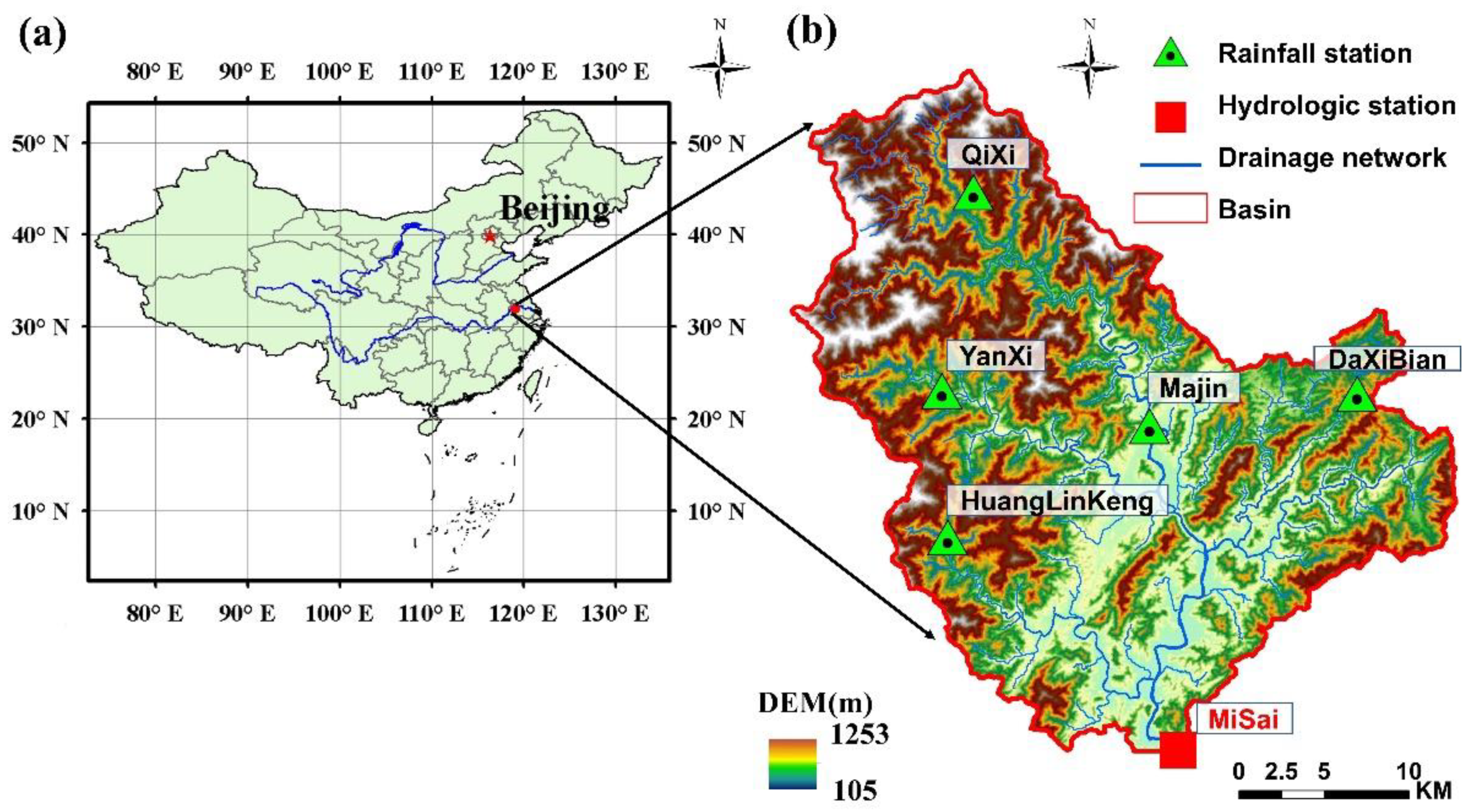
Figure 1. Location of Misai watershed and relevant hydrological information ((a) Location of Misai watershed; (b) Hydrological information of Misai watershed).
Water 14 02854 g001
Figure 2. Adopted flowchart of the study and Schematic diagram of different land-use areas and soil layers in the watershed (ae represent different land-use areas, h is the depth of litter layer, D is the thickness of aeration zone, and P is rainfall).
Water 14 02854 g002
Figure 3. The simulation results on daily scale. Scatterplots of the simulated discharge against the observed discharge under calibration (a) and validation (b) period (the dashed line represents a straight line with a slope of 1, and the linear regression line is the solid line, shaded is 90% confidence band). The results of model assessment are (c) Nash–Sutcliffe efficiency (NSE). The red dotted line represents the dividing lines where the results are “satisfactory” to “good”, the yellow are “good” to “very good”. (d) Percent bias error (BE). The red dotted line represents the dividing lines where the results are “unsatisfactory” to “satisfactory”, the yellow are “satisfactory” to “good” and the cyan are “good” to “very good”. (e) Kling–Gupta Efficiency (KGE).
Water 14 02854 g003
Figure 4. The simulation results on daily scale. (a) Observed and simulated hourly discharge (occurred on 2 April 1982; 5 May 1985; 19 May 1986; 26 May 1987 in turn, OBQ: observed values). (b) Boxplot graph of evaluation results (BE, PE and ARPT are absolute values).
Water 14 02854 g004
Figure 5. Mean absolute error (MAE) of monthly simulated discharge.
Water 14 02854 g005
Figure 6. The distribution of evaluation results under different types of floods (in turn: NSE, KGE, BE, PE). The point size represents different flood discharge.
Water 14 02854 g006
Figure 7. Simulated changes with different factor changes. (a) Impact of the different factors change on the relationship between rainfall and runoff. The lines above and below the L-WSCC line represent different directions of influence on runoff, and the intervals between the lines with the same color indicate the degree of influence of different factors on runoff. (b) The ΔMAE in different scenarios.
Water 14 02854 g007
Table 1. Rate of land-use change of the study area from 1982 to 1988.
Year19821983
(%)
1984
(%)
1985
(%)
1986
(%)
1987
(%)
1988
(%)
Land Use
Cultivated land-−18.4126.002.53−42.4223.1212.83
Forest land-2.31−8.03−0.0116.00−8.047.05
Grass land-753.00−14.391.4826.5251.92−99.42
Water-1.67−0.96−2.571.882.42−0.73
Urban land-−38.15110.17−45.9014.2914.17−45.83
Publisher’s Note: MDPI stays neutral with regard to jurisdictional claims in published maps and institutional affiliations.