Article

A Comprehensive Approach to Develop a Hydrological Model for the Simulation of All the Important Hydrological Components: The Case of the Three-River Headwater Region, China

1
Key Laboratory of Water Cycle and Related Land Surface Processes/Institute of Geographic Science and Natural Resources Research, Chinese Academy of Sciences, Beijing 100101, China
2
Qinghai Key Laboratory of Basin Water Cycle and Ecology, Qinghai Institute of Water Resources and Hydropower, Xining 810001, China
*
Author to whom correspondence should be addressed.
Water 2022, 14(18), 2778; https://doi.org/10.3390/w14182778
Submission received: 19 July 2022 / Revised: 27 August 2022 / Accepted: 2 September 2022 / Published: 7 September 2022
(This article belongs to the Special Issue Modelling Hydrologic Response of Non-homogeneous Catchments II)

Abstract

:
The objective of the study was to configure the Hydrological Modeling System (HEC-HMS) in such a way that it could simulate all-important hydrological components (e.g., streamflow, soil moisture, snowmelt water, terrestrial water storage, baseflow, surface flow, and evapotranspiration) in the Three-River Headwater Region. However, the problem we faced was unsatisfactory simulations of these hydrological components, except streamflow. The main reason we found was the auto-calibration method of HEC-HMS because it generated irrational parameters, especially with the inclusion of Temperature Index Method and Soil Moisture Accounting (an advanced and complex loss method). Similar problems have been reported by different previous studies. To overcome these problems, we designed a comprehensive approach to estimate initial parameters and to calibrate the model manually in such a way that the model could simulate all the important hydrological components satisfactorily.

1. Introduction

Understanding how water is used and cycled through a watershed provides the foundation for understanding and describing the interactions of landscapes and water. The most basic tool for understanding these interactions is the water cycle [1]. The water cycle is one of the most important cycles (e.g., carbon cycle, the nitrogen cycle, and other biogeochemical cycles) of Earth’s climate system [2,3] and comprises different hydrological components such as precipitation, evaporation, transpiration, soil water, and streamflow [1]. Therefore, for precise water resources management and planning and sustainable development for a region, it is essential to study all the important components (e.g., precipitation, evaporation, transpiration, soil water, baseflow, streamflow, snowmelt, and terrestrial water storage) of the water cycle [4,5]. However, the observed data of these components, except precipitation and streamflow, are hardly available because they are difficult to measure for longer periods and larger watersheds [6,7]. For the past two decades, hydrological models have become the most powerful tools to study these hydrological components [8,9]. However, their performance is mainly dependent on the calibration, which is the most important and central process in the development of a model [10,11]. Generally, calibration methods are divided into two categories: manual and automatic [12]. In manual calibration, parameters are adjusted manually to achieve an objective function (e.g., the minimization of root mean square error). However, this is time-consuming, subjective, and tedious, especially when the number of parameters increases, and requires expertise in the field of hydrology and modeling [9,12,13].
Recently, auto-calibration has become mainstream for solving the issues of optimizing the model’s parameters [9,14]. These computer-aided methods automatically search a set of optimal parameters to some predefined criteria (e.g., percent error in peak) [15]. Additionally, these methods are considered objective, speedy, and relatively easy to implement [9,16]. Although intensive advancement has been made in auto-calibration, most applications have been restricted to research and not operational modeling [17], and still many problems have been reported by researchers, especially related to the reliability of calibrated parameters [18,19,20,21]. Similar problems were faced in this study when we tried to calibrate the Hydrological Engineering Center–Hydrological Modeling System (HEC-HMS) automatically using built-in optimizing techniques in the Three-River Headwater Region (TRHR). According to Bashar and Zaki [22] and Dariane, Javadianzadeh and James [14], the optimization methods (i.e., Nelder–Mead and Univariate Gradient) used in HEC-HMS are either inefficient or do not work rationally, especially with the inclusion of Soil Moisture Accounting (SMA) and Temperature Index Method (TIM). Therefore, many studies, such as, Bhuiyan, McNairn, Powers and Merzouki [18], Chea and Oeurng [23], Fleming and Neary [24], Gebre [19], Gyawali and David [25], Koch and Bene [20], and Neary, et al. [26] suggested using both the automated and manual (preferably) methods during calibration of HEC-HMS when using SMA and TIM, because the parameters obtained by the automated methods are mostly irrational, which yields misleading results [21,22].
As mentioned above, many studies suggest using manual calibration; however, we could not find any comprehensive approach that can be used to configure HEC-HMS in such a way that it can be used to generate all the important hydrological components satisfactorily. Moreover, these studies focused only on the simulation of streamflow. Therefore, in this study, we designed a comprehensive approach to configure HEC-HMS for the simulation of all the important hydrological components (e.g., streamflow, baseflow, soil moisture, snowmelt water, evapotranspiration, and terrestrial water storage) satisfactorily. The focus of the approach was to provide a way to estimate some logical initial values for the process parameters, explore the sensitive parameters, and determine the relationships between parameters and hydrograph components, e.g., which parameter affects which hydrograph component (e.g., low flow, high flow, rising limb, and falling limb). This not only can reduce the time of calibration but also enhance the understanding of the hydrological processes and provide some rational parameters and, consequently, some reasonable results. Additionally, this approach can be applied to similar kinds of hydrological models (e.g., SWAT, TOPMODEL, and HBV) when it is necessary to simulate all the important hydrological components of the hydrological cycle of a region.

2. Materials and Methods

2.1. Study Area

The Three-River Headwater Region (TRHR) is the source region of the Lancang, Yellow, and Yangtze Rivers located in the Qinghai Tibetan Plateau (QTP), China (Figure 1). The source region of the Yangtze River (SYAR) above the Zhimenda streamflow gauge, the source region of the Yellow River (SYER) above Tangnaihai, and the source region of the Lancang River (SLR) above Xiangda contribute areas of 54% (158,027 km2), 40% (117,755 km2), and 6% (16,919 km2), respectively, to the TRHR [27], which covers a total area of 292,700 km2. It extends between 32°–36° N and 89°–103° E, with an elevation ranging from 2600 to 6600 m AMSL (Figure 1). The TRHR is considered the water tower of China and is an important nature reserve situated in QTP [28]. The region has a very complex topography, with highly elevated mountains as the basic structure of the landscape [29]. The region has a harsh and dry climate, with temperature ranging from −5.6 °C to 7.8 °C and precipitation stretching between 262 mm and 772 mm [28,30].

2.2. Data Description

The observed daily streamflow data of 5 hydrometric stations (i.e., Zhimenda, Xiangda, Jimai, Maqu, and Tangnaihai) were obtained from the Hydrology and Water Resources Survey Bureau of Qinghai province for the period 1980–2015 (Figure 1). Meteorological data (i.e., precipitation, maximum temperature, minimum temperature, wind speed, solar radiation, and relative humidity) of 23 climate stations (Figure 1) were obtained from the Qinghai Meteorological Bureau (QMB) for the period 1980–2015. All data (e.g., climate, discharge, elevation, soil, land cover, soil moisture, and water storage) required for this study were obtained from different sources, and data name, temporal resolution, spatial resolution, available period, and sources are described in Table 1.

2.3. Setup of HEC-HMS

The Hydrological Modeling System (HEC-HMS), developed at the Hydrologic Engineering Centre (HEC) [44], has been applied around the world for flood modeling [45], water resource assessment [46], climate change impacts assessment [47], urban flooding [48], and streamflow simulation [49]. HEC-HMS encompasses seven methods to calculate precipitation losses (e.g., deficit and constant loss and SMA), seven transformation methods (e.g., Soil Conservation Services and Clark Unit Hydrograph), five baseflow estimation methods (e.g., Linear Reservoir and Recession methods), and six routing methods (e.g., Muskingum). There are two methods (i.e., Simple and Dynamic Canopy) to estimate interception and transpiration through plants, and a method to estimate water stored in surface depressions [44].
In this study, Thiessen Polygon, Penman–Monteith, TIM, SMA, Clark Unit Hydrograph, Muskingum Channel Routing, Linear Reservoir Baseflow Method, Dynamic Canopy, and Simple Surface Storage were included in the setup of HEC-HMS. The above-mentioned methods are elaborated in detail in the Supplementary Materials.
Thiessen Polygon was applied to interpolate daily climate data over each sub-basin (created in Section 2.4.1). This method is useful when gauges are scarce in a basin as compared to the basin area, as in Meenu, et al. [50]. For snowmelt modeling, each sub-basin was divided into different elevation bands (ranging from 3 to 5) for proper application of TIM.

2.4. Calibration and Validation

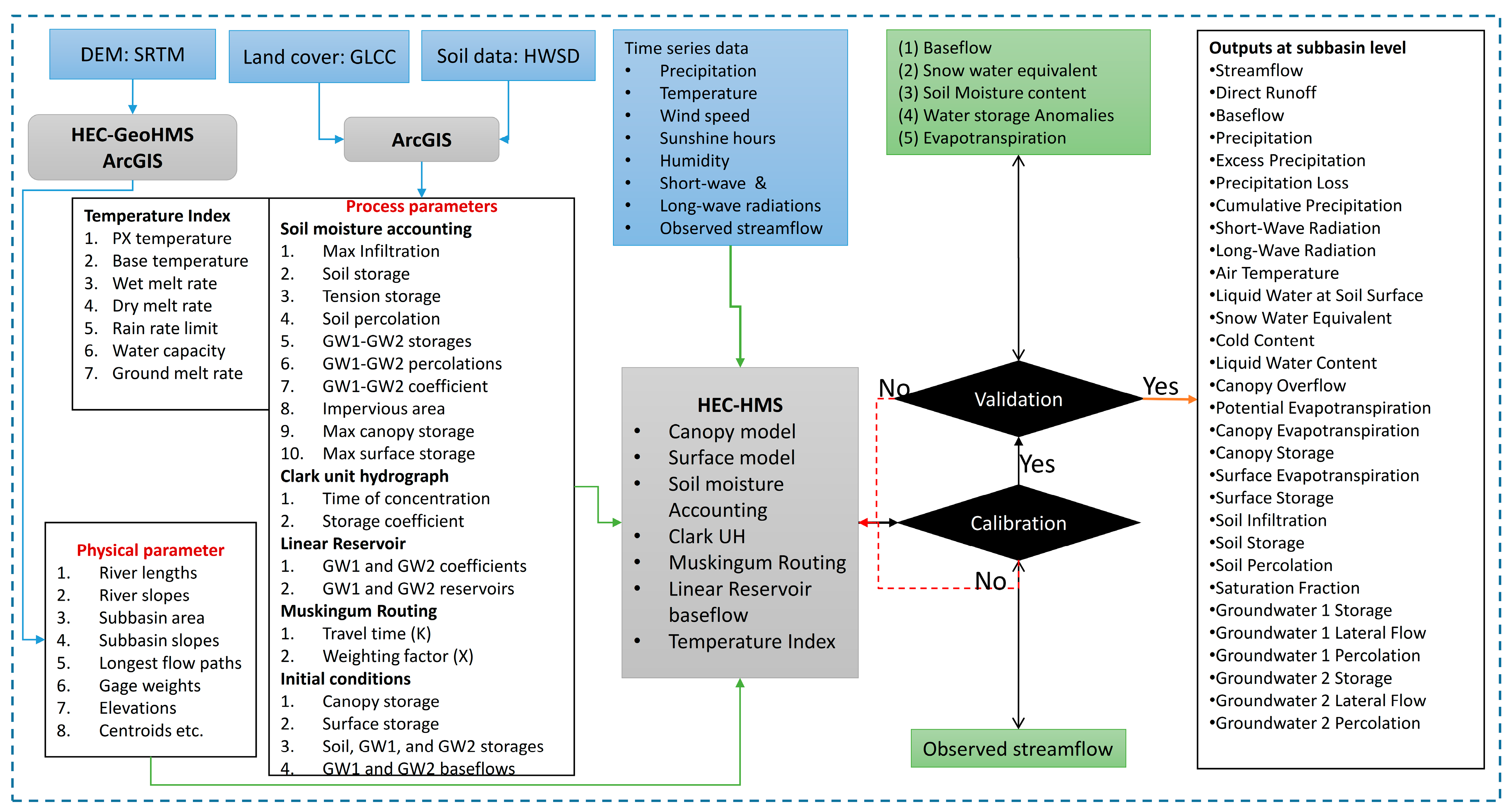
The auto-calibration does not provide optimal results and rational parameters in HEC-HMS, especially with TIM and SMA [21,22], and when we need to simulate other hydrological components such as soil moisture and snow water equivalent. Therefore, for the generation of all-important hydrological components, we adopted the manual calibration process in this study. For this purpose, we designed a comprehensive approach for the development of HEC-HMS, which can reduce time and easily manage many parameters. The whole procedure for the development of HEC-HMS is shown in Figure 2, which shows the required input data, tools used, model parameters, methods, and possible outputs, and is elaborated in the following steps.

2.4.1. Estimation of Physical Parameters

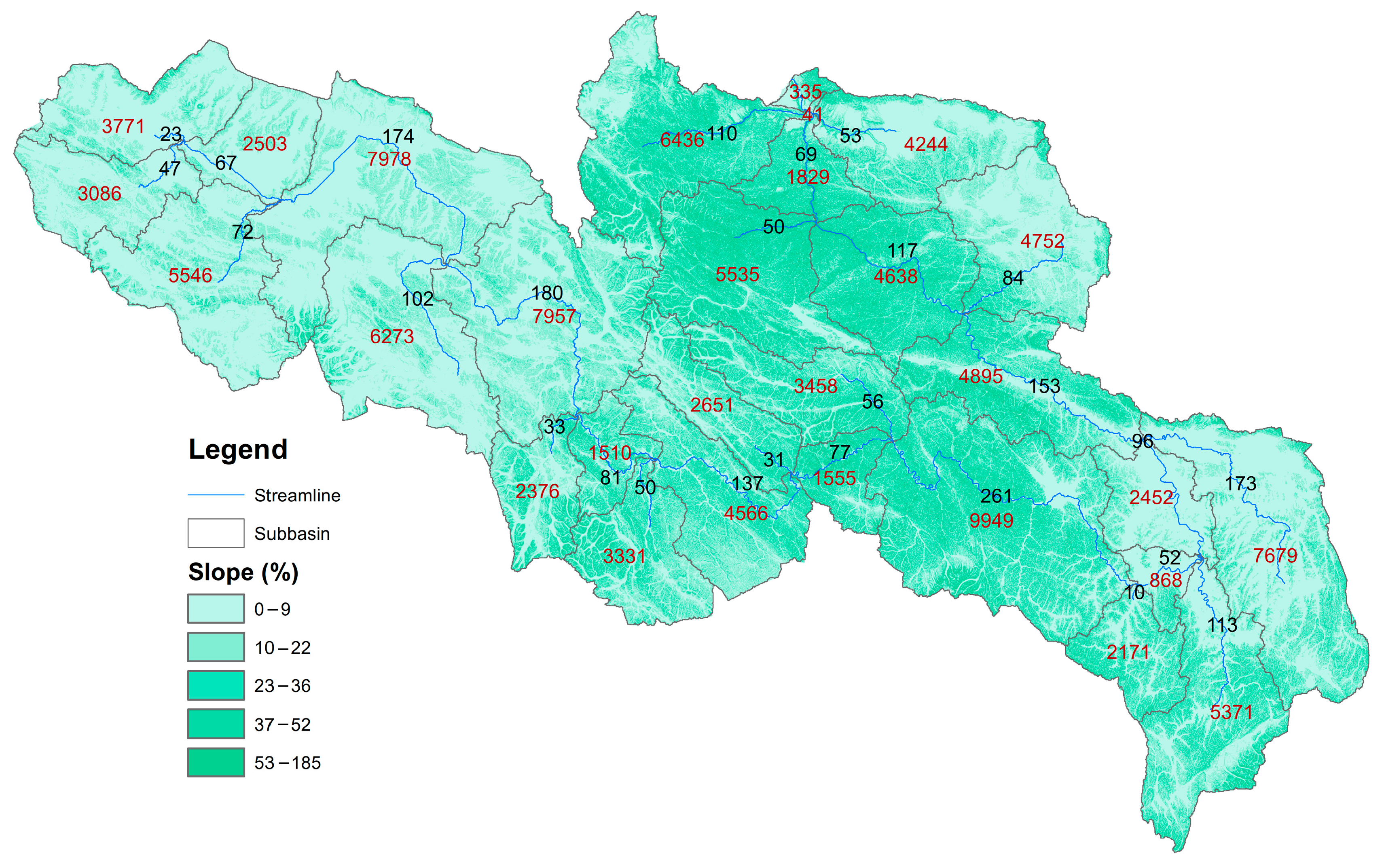
One of the tedious and time-consuming but important steps in the development of a complex hydrological model is to prepare input data [51], which can generally be divided into time-series data (e.g., climatic and hydrometric) and model parameters. The model parameters are of two kinds: physical parameters and process parameters [9,52]. Physical parameters represent the physical characteristics of watersheds [52], which are obtained by the watershed delineation that is considered the first step in hydrological modeling [53]. The delineation divides a basin into small sub-basins or grids, and their topographic characteristics such as sub-basin area, river length, sub-basin slope, and river slope are calculated. In this study, the TRHR was divided into 82 sub-basins (44 for SYAR, 29 for SYER, and 9 for SLR) during the delineation process of 90 m-SRTM-DEM [31], and physical characteristics were estimated for each sub-basin, as shown in Figure 3.

2.4.2. Estimation of Process Parameter

Generally, process parameters cannot be measured directly from the watershed, and these parameters need to be estimated indirectly through calibration [52]. To start the calibration process, some initial values of these parameters are required [9]. Sometimes, these initial values are assumed in cases when there is a simple model setup, with a very limited number of process parameters, and when we do not need a high level of satisfaction and must simulate only streamflow. However, this still requires a high level of expertise in the field. On the other hand, in the case of a very complex model setup including many parameters, it is essential to estimate some logical initial values of these parameters. This will not only help to simulate satisfactory hydrological components but also reduce the time of calibration. Additionally, this will provide rational and logical calibrated parameters. Therefore, in this study, we estimated these parameters in a systematic way.
The SMA method requires 5 initial conditions (i.e., canopy storage, surface storage, soil storage, groundwater layer 1 (GW1) storage, GW2 storage) and 13 process parameters (i.e., maximum infiltration, soil storage, tension storage, soil percolation, GW1 storage, GW1 percolation, GW1 coefficient, GW2 storage, GW2 percolation, GW2 coefficient, impervious surface area, maximum canopy storage, maximum surface depression storage), as described in Figure 2 [44]. The initial canopy and surface storages were taken as 0%, assuming no precipitation occurrence for a long time, as in Ahbari, et al. [54], and the rest were set as 30%. The initial values can be taken from 0% to 100%, with 0% showing almost no water available at the start of the simulation [25]. In the case of taking 0% as the initial conditions, a longer period (e.g., 5–10 years) will be required as a model spin-up period. In this study, we used 3 years of daily data as a spin-up (warm-up) period to reach the model at a steady state.
In contrast to the initial conditions, we need some reasonable and logical values for process parameters before starting the calibration process. These are estimated by using soil data and LCLU for each sub-basin on overage basis [2,22,25]. In this study, we used HWSD (Table 1) to extract soil properties such as depth and texture for the region. The soil texture is mainly used to identify the soil properties [24] because the variability in soil moisture patterns is most closely related to the variability in soil texture as compared to other soil properties [55]. Sandy loam and loam soil are dominant soil types in the SYER, covering an area of about 61% and 34% of the total area, respectively (Table 2). Porosity, field capacity, and saturated hydraulic conductivity (Table 2) were obtained from the literature, such as Clapp and Hornberger [56], J. Rawls, et al. [57], and Saxton and Rawls [58], using the soil texture of the region. The infiltration rates mentioned by FAO [59] against the texture of soil were assigned as initial values for maximum infiltration, and hydraulic conductivity as initial values for soil, GW1, and GW2 percolations, as in Fleming and Neary [24]. Soil and tension storages were estimated by multiplying the soil depth with porosity and field capacity, respectively, as in Ahbari, Stour, Agoumi and Serhir [54] and Samady [60]. The storage coefficients and storage depths of GW1 and GW2 were estimated using recession analysis on the observed streamflow, described in Fleming and Neary [24] and Samady [60]. The following steps were used to estimate the storage coefficients and storage depths of GW1 and GW2:
  • First, search and separate single isolated storm event from streamflow time series.
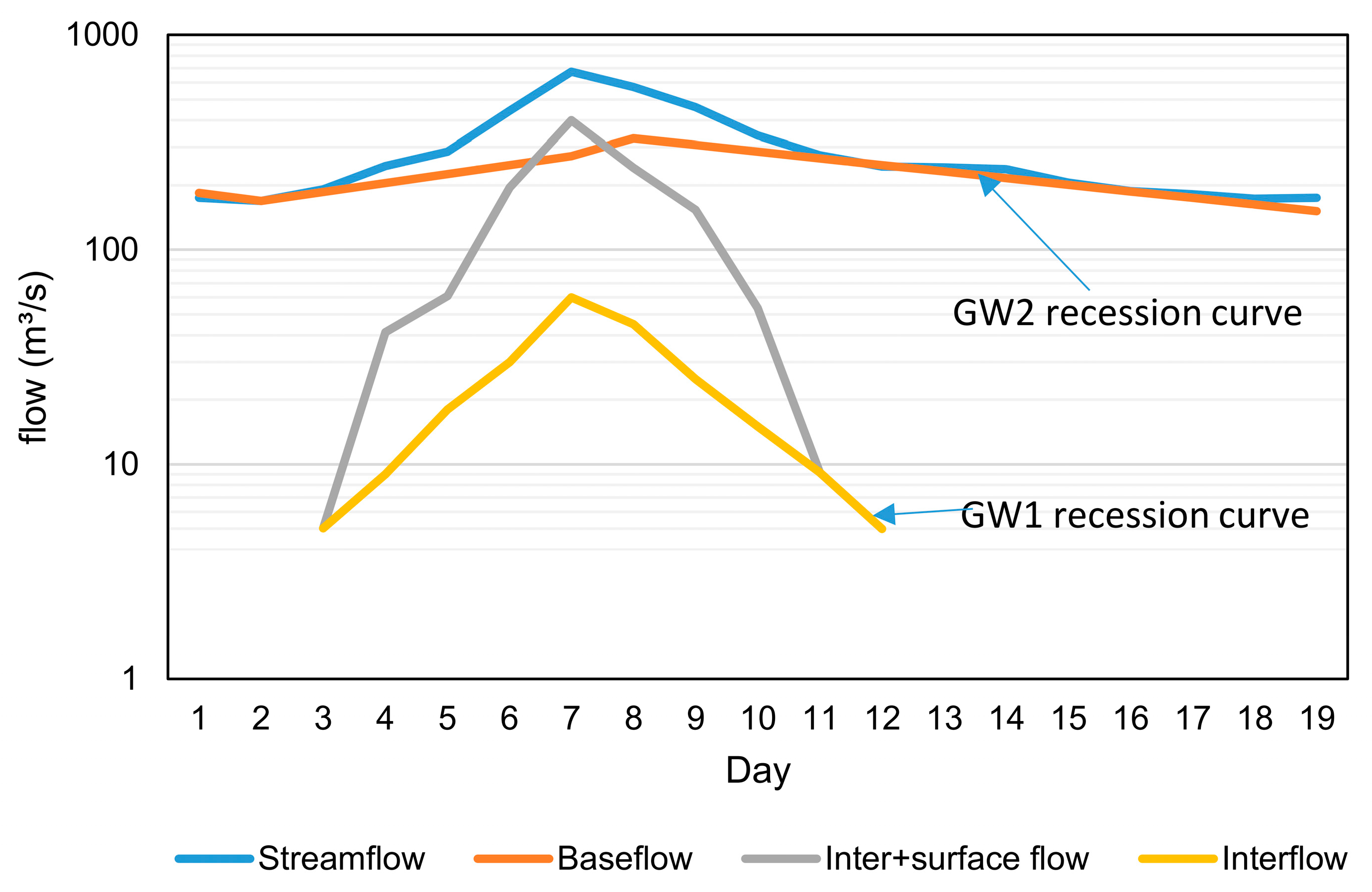
  • Plot a streamflow hydrograph for a single isolated storm event on a semi-logarithmic graph, as shown in Figure 4.
  • Separate the baseflow and interflow from the streamflow hydrograph. We used the graphical method [61] for the separation of hydrograph components (Figure 4), as in Ahbari, Stour, Agoumi and Serhir [54] and Samady [60].
  • Estimate the recession constant (k) for both the recession curves of baseflow and interflow. We used regression analysis on a semi-logarithmic graph. Baseflow is contributed by the deep groundwater layer (GW2) and interflow from the shallow groundwater layer (GW1) [24].
  • Estimate the storage coefficient (Sc), storage capacity (St), and storage depth (St/area) with the following equations for both GW1 and GW2:
S c = 1 l n K
S t = S c × Q t = 1 l n K Q t
Q t = Q o K t  
where Qo represents the initial baseflow (t = 0) and Qt is the baseflow at time t (day). Equation (2) is the integration of the recession equation (Equation (3)) to estimate the storage capacity of a watershed. Similarly, estimate Sc and St for different storms in different seasons, where no rain occurs for some time after the peak flow [24]. The main step in the recessional analysis is to determine the recession constant. Typically, it ranges from 0.7 to 0.94 for interflow and 0.93 to 0.995 for baseflow [62]. However, a high value (e.g., >0.9) indicates the dominance of baseflow in a watershed [63]. In this study, we determined recession constants ranging between 0.92 and 0.98 for baseflow and between 0.6 and 0.88 for interflow. This procedure was applied to 5 gauging stations (Tangnaihai, Maqu, Jimai, Zhimenda, and Xiangda) and used for each sub-basin because data are available only on these stations. However, the exact values were estimated after calibration and validation processes.
Table 2. Soil properties in the source region of the Yellow River.
Soil TextureArea (km2)% of the Total AreaSoil Depth (mm)Porosity (cm3/cm3)Field Capacity (cm3/cm3)KS (mm/h)Infiltration (mm/h)
Clay2481210000.490.410.62
Clay loam1926210000.480.362.35
Loam40,205346540.460.2813.210
Sand630110000.40.121025
Sandy loam72,088613000.440.1825.920
Silt loam670110000.490.316.87
Note(s): Sources: FAO (infiltration) [57,58], HWSD [33].
Figure 4. Hydrograph components to estimate recession constant for GW1 and GW2 layers.
Water 14 02778 g004
The impervious surface area was obtained from the NASA Socioeconomic Data and Applications Center [64], which was only 0.09% of the total area of the SYER, and even less (0.03%) has been mapped by Zhang, et al. [65]. Max canopy (Table 3) and surface-depression storages (Table 4) were obtained from the literature, such as Ahbari, Stour, Agoumi and Serhir [54], Samady [60], and Verbeiren, et al. [66], using the vegetation types and basin slope in the region. Vegetation types were extracted using Global Land Cover Characteristics (Table 1), with 88% of grassland, and the slope was extracted using SRTM-DEM (Table 1), ranging from 0% to 185% (17% mean) in the SYER (Figure 3).
The LRBM requires 3 parameters (i.e., initial baseflow, groundwater coefficient, and reservoir) for each GW layer. Initial baseflow can be easily estimated from the observed streamflow, which can be low flows of streamflow, as used in this study. The groundwater coefficient, which is a response time of a basin [21], is the same as described above for SMA. Reservoirs are used to attenuate the streamflow; the greater the number of reservoirs, the more attenuation in the streamflow [44]. There are two parameters for the CUH method: time of concentration (TC) and basin storage coefficient. TC was estimated using a built-in function in HEC-GeoHMS, named the TR55 method, in which a basin (sub-basin) is divided into three flows such as sheet flow over the plane surface, shallow flow in small streams, and open channel flow. This requires much data about land and channel characteristics (e.g., land slope, land cover, width, depth, velocity, and roughness coefficient) for precise estimation of TC, which does not seem possible for a large and remote area. Nonetheless, we used Google Earth to measure the channel characteristics (e.g., cross-sectional area) at different locations to make an informed guess about TC. A detailed description of the TR55 method is given in [67]. The storage coefficient represents the temporary storage of excess precipitation in the basin as it drains to the outlet point [68], which can be computed as the flow at the inflection point on the falling limb of the hydrograph divided by the time derivative of flow [69]. Muskingum routing requires two parameters to estimate: K and X [44]. K is the travel time of a flood wave through a reach. Therefore, if inflow and outflow hydrographs are available, it can be estimated as the interval between similar points on inflow and outflow hydrographs (e.g., the centroid areas of two hydrographs) [23]. X is a dimensionless weighting factor, which ranges between 0 and 0.5 [44,70].

2.4.3. Sensitivity Analysis

After preparing input data and before calibration, another key process in manual calibration is to explore the sensitive parameters. Sensitivity analysis (SA) helps to recognize the parameters that have strong effects on the model outputs and hence influence the model response. SA also supports analyzing the interaction between parameters, its preferable range, and its spatial variability, which in turn influence the model outcomes. Consequently, SA accelerate the calibration process in hydrological modeling [71]
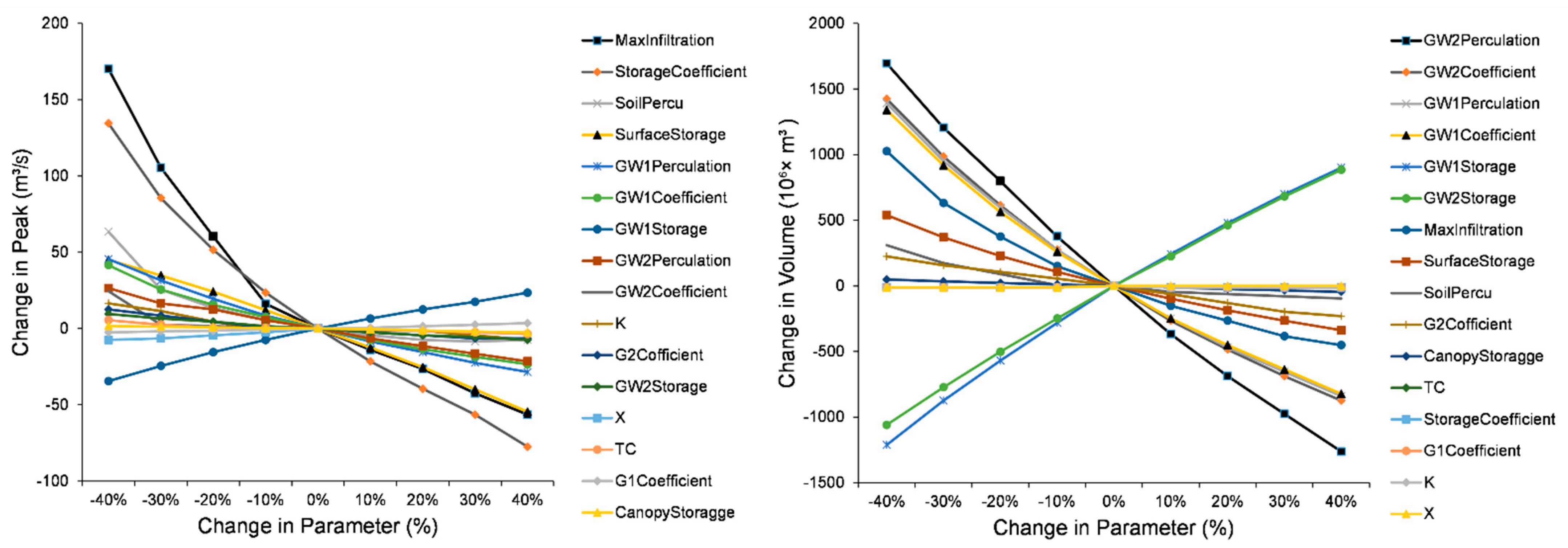
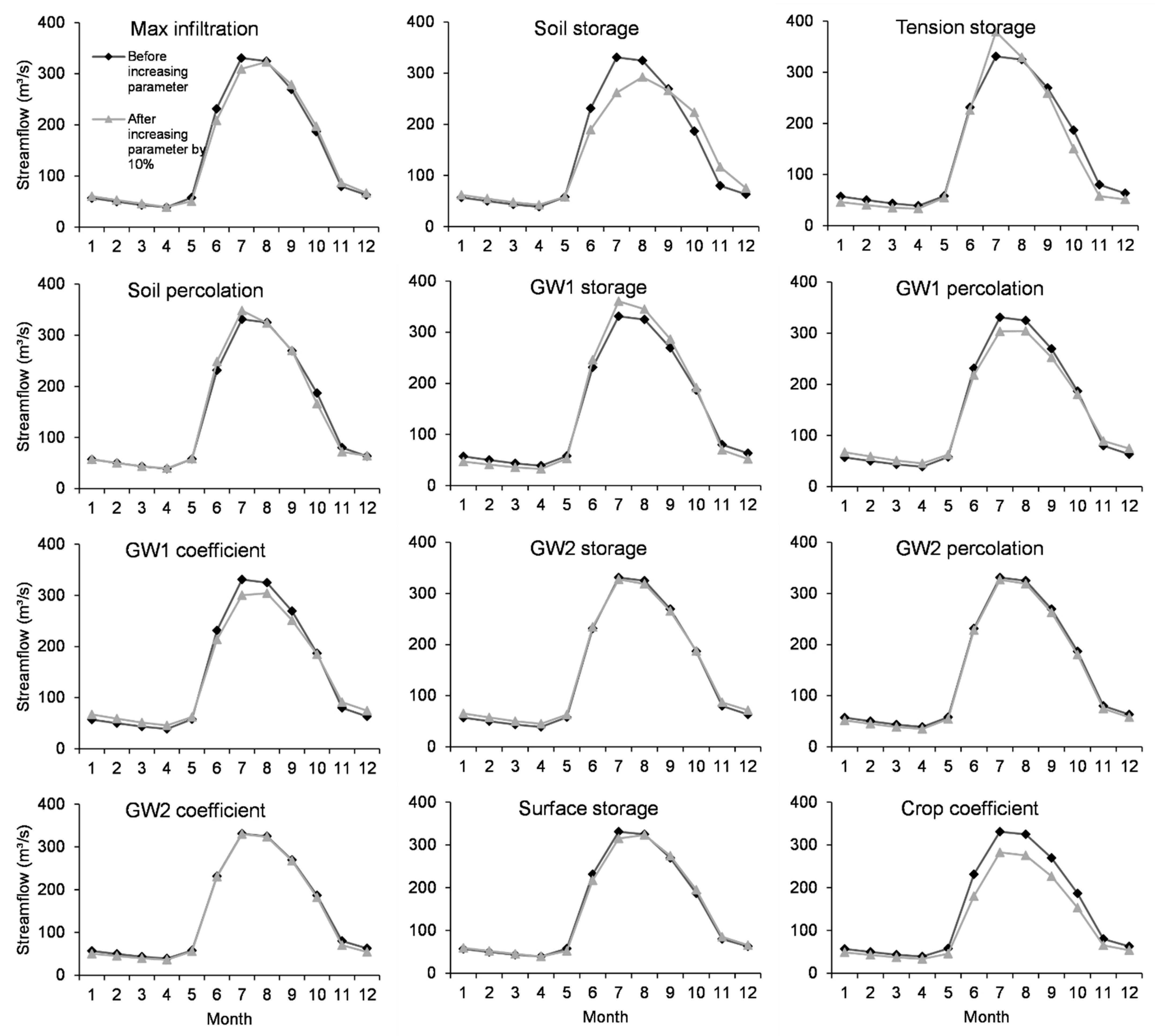
For this purpose, we used the local sensitivity analysis to determine the sensitive parameters in the region. According to [72], there are two types of sensitivity analysis: local and global. In the local, each parameter is changed one by one while keeping all other parameters unchanged, and its impact is measured on outputs. On the other hand, in the global, a model is run with the initial values of parameters, the changes in parameters and output are measured, and the percentage effect of each parameter on the output is calculated to determine the sensitive parameters. Sensitivity analyses were carried out by changing each parameter by 10% each time (between −40% and +40%) to observe the changes in simulated discharge. Two indicators, peak flow (PF) and total flow volume (TFV), were used to observe the effect of each parameter on discharge. All the parameters were ranked from top to bottom (the most sensitive to the least sensitive) and shown in Figure 5. In the case of PF, the top four sensitive parameters were maximum infiltration, storage coefficient, soil percolation, and surface storage; in the case of TFV, they were the percolations and storage coefficients of GW1 and GW2. This showed that maximum infiltration was most sensitive in the case of PF and percolation of GW2 in the case of TFV in the SYER. Instead of observing the parameter effects on PF and TFV, we also detected the parameter’s effects on other hydrograph components such as the rising limb, falling limb, and low flows. For this purpose, each parameter was increased by 10% (one by one) and its impact was observed on the hydrographs, which are shown in Figure 6. This gave a clear picture of which parameters affected which components of the hydrograph and made it easy to calibrate the model accurately.
In this study, HEC-HMS was calibrated for 2006–2010 and validated for the forward period (2011–2015) and the backward period (1981–2005) at Jimai, Maqu, Tangnaihai, Zhimenda, and Xiangda hydrometric stations. The other hydrological components such as soil moisture, baseflow, and TWS were validated for the periods that were available. For the evaluation of calibration and validation, four commonly used indicators (i.e., coefficient of determination (R2), Nash–Sutcliffe efficiency (E), normalized root mean square error (NRMSE), and percent volume deviation (PVD)) were used along with graphical plots, as in García, et al. [73], Mahmood, et al. [74], Meenu, Rehana and Mujumdar [50], and Verma, et al. [75].
R 2 =   ( Q o b s   Q o b s ¯ ) × ( Q s i m   Q s i m ¯ )   ( Q o b s   Q o b s ¯ ) 2 × ( Q s i m   Q s i m ¯ ) 2
P V D   ( % ) = 100 × Q s i m Q o b s Q o b s  
E = 1   ( Q s i m   Q o b s ) 2   ( Q o b s   Q o b s ¯ ) 2  
N R M S E = R M S E Q o b s ¯ =   ( 1 n i = 1 n ( Q s i m Q o b s ) 2 )   Q o b s ¯

2.5. Baseflow Separation

Baseflow is one of the most important parameters of a hydrological cycle, contributing a large part to streamflow, but it is difficult to measure [6]. Many baseflow separation methods (graphical and digital filters) have been developed to estimate baseflow from the streamflow, which are described in [62,76,77]. Since observed baseflow is not available in the TRHR, and we need to evaluate baseflow simulated by HEC-HMS, we applied a frequently used digital filter known as the recursive digital filter described by Nathan and McMahon [62], as below:
f k = α f k 1 + ( 1 + α ) 2 [ y k y k 1 ]
where f k is quick flow at the kth time, α is a filter parameter, and y k is streamflow. Nathan and McMahon [62] recommended an α value of 0.925 for daily flow and 0.995 for hourly flow. In the present study, daily streamflow was used in the TRHR.

2.6. Terrestrial Water Storage

Terrestrial water storage (TWS) change is crucial for global as well as regional hydrological cycles and water resources management [78]. It is also essential for understanding a wide range of hydrological, climatological, and ecological processes. TWS mostly includes surface water, snow and ice, soil moisture, and groundwater storage. However, it is difficult to measure TWS directly [7]. In the present study, we used a hydrological model (i.e., HEC-HMS) to estimate the TWS in the TRHR. In the present study, TWS included canopy storage ( S c a n o p y ) , surface storage ( S s u r f a c e ) , soil storage ( S s o i l ) , groundwater storages from GW1 and GW2 ( S g r o u n d 1 , S g r o u n d 2 ) , and water stored in snow and ice as SWE ( S s w e ) , as below:
T W S = S c a n o p y + S s u r f a c e + S s o i l + S g r o u n d 1 + S g r o u n d 2 + S s w e  
Since the in situ observations of TWS are not available in the TRHR, remote sensing data constitute a good source to evaluate TWS obtained by HEC-HMS. For this purpose, we obtained GRACE data of three solutions, i.e., GFZ, TU-CSR, and TU-CSR-Mascon for the period 2002–2015. TWS from GRACE is in the form of anomalies relative to 2004–2009. Therefore, we also calculated anomalies of TWS relative to 2000–2009 for a proper comparison.

2.7. Actual Evapotranspiration Estimation

Evapotranspiration is one of the most important components of the hydrological cycle and one of the most important physical processes in natural ecosystems. It links water and energy between the soil, land surface, and the atmosphere in the climate system [79,80]. The estimation of actual evapotranspiration (AET) is of vital importance in hydrological modeling, water resources management and planning, and related ecosystem services, as well as in addressing global climate change [79,81]. Evapotranspiration is also important for predicting plant productivity and species richness [80]. In the present study, the water balance equation was used to estimate AET, as given below:
A E T = P Q s i m Δ S  
where P, Qsim, and ΔS represent precipitation, simulated flow, and changes in water storage, respectively, in the basin. ΔS is generally assumed negligible for analysis in a longer period (≥10 years) [82] because it is difficult to measure. Nonetheless, in the present study, ΔS was estimated from TWS, as below:
Δ S = T W S t T W S t 1

3. Results

3.1. Calibration and Validation with Streamflow

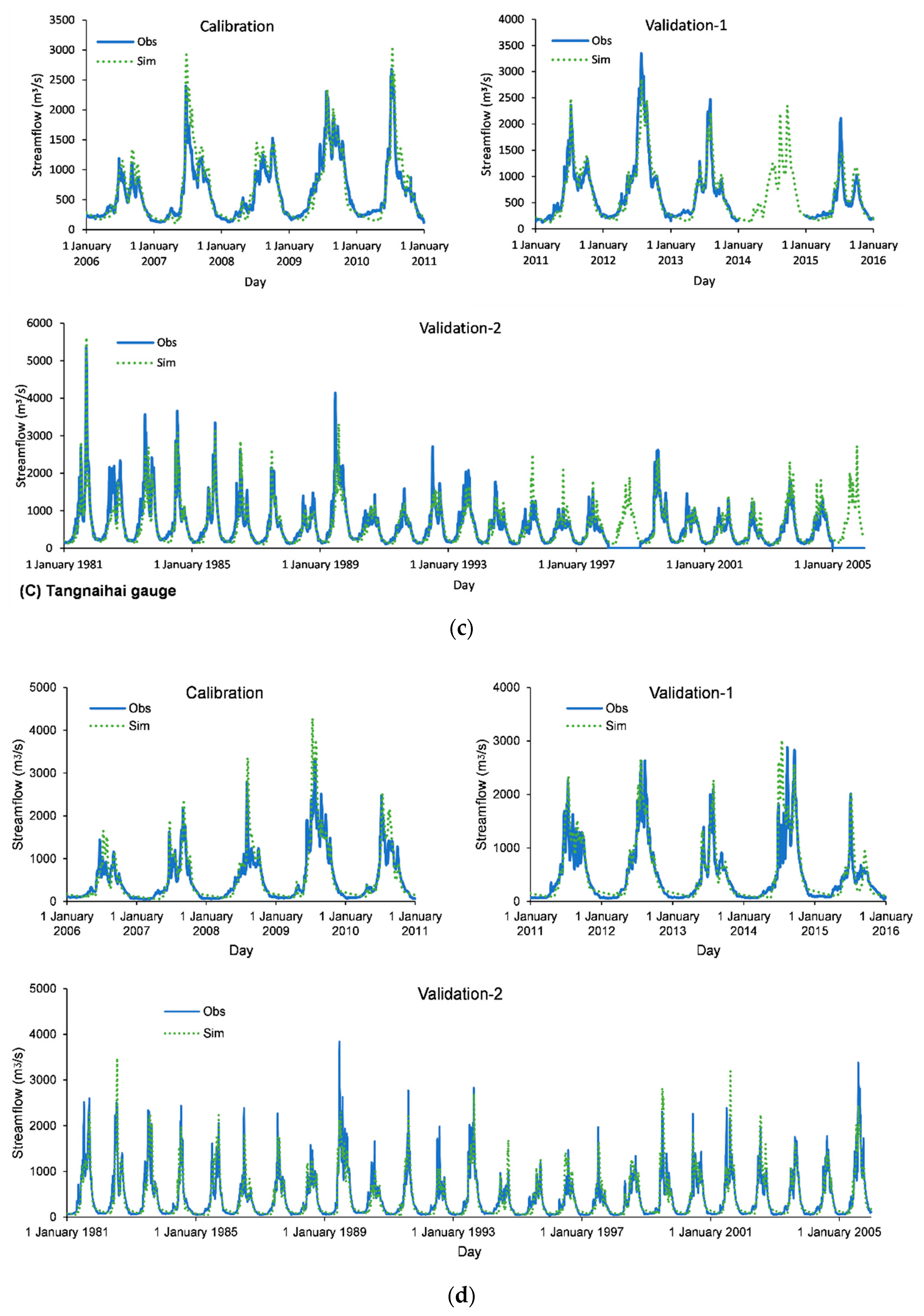
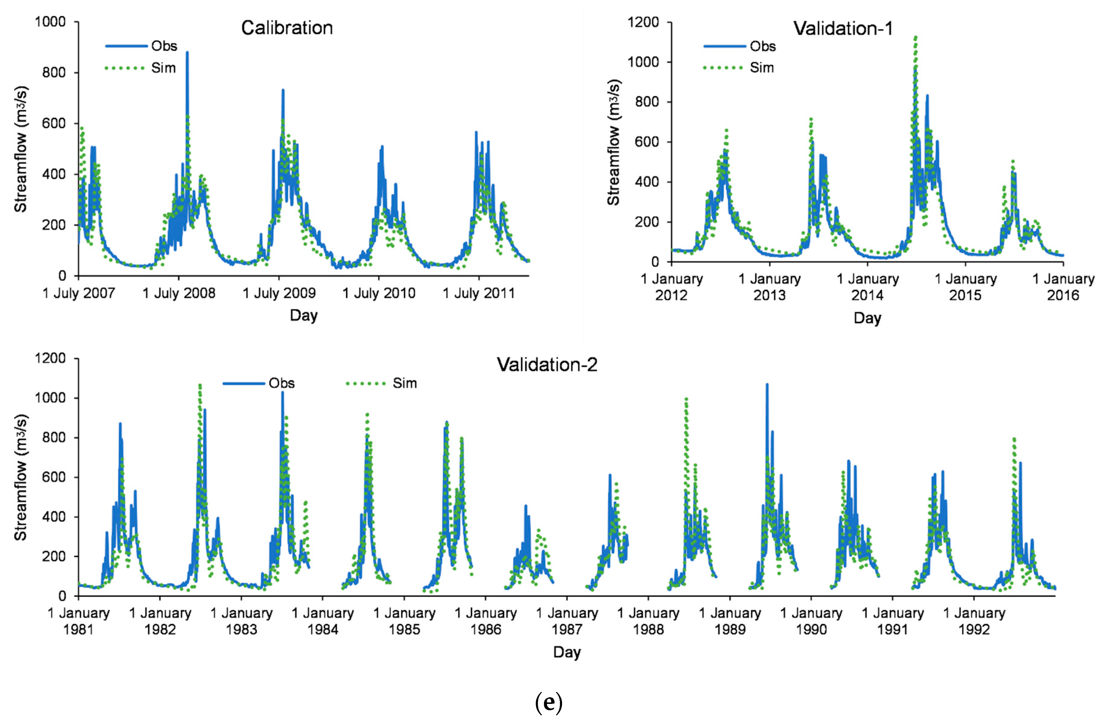
Table 5 describes the results of calibration and validation obtained from daily simulated and observed streamflow at five hydrometric stations. The E values ranged from 0.66 to 0.85 during calibration, 0.69 to 0.90 for validation-1, and 0.62 to 0.82 for validation-2. The results of R2 were almost similar or slightly better than the E results during both calibration and validation. The PVD values varied between −4.5% and 9.0% for calibration, −1.5% and 13% for the first validation period, and −4.5% and 21% for the second validation period. On the other hand, NRMSE varied from 0.30 to 0.51 during calibration, 0.27 to 0.49 during validation-1, and 0.40 to 0.52 during validation-2. According to Van Liew and Garbrecht [83], E values greater than 0.75 are greatly appreciated, and the values between 0.36 and 0.75 are referred to as satisfactory depending on the objectives of the study. The model showed acceptable results on all gauges, though the numbers of climate stations are sparse, especially in the SYAR. Similar results have been reported by Meng, et al. [84], Yang, et al. [85], and Zhang, et al. [86] in the SYER. For example, E values ranging from 0.78 to 0.91 for calibration and 0.70 to 0.89 for validation at Tangnaihai have been reported by Meng, Su, Yang, Tong and Hao [84], Yang, Wang, Yu, Krysanova, Chen, Schwartz and Sudicky [85], and Zhang, Su, Hao, Xu, Yu, Wang and Tong [86]. Furthermore, E values ranging from 0.67 to 0.81 for calibration and 0.61 to 0.78 for validation at Maqu and from 0.51 to 0.76 for calibration and 0.49 to 0.61 for validation at Jimai have been reported by Meng, Su, Yang, Tong and Hao [84]. Guo, et al. [87], Wang, et al. [88], and Zhang, et al. [89] also showed similar results of calibration and validation for the SYAR and SLR, ranging from 0.72 to 0.87.
The graphical presentation of results is another important visual tool for the evaluation of model performance subjectively and qualitatively, showing how well simulated data follow the variations (e.g., peak and low flows) in observed data. Therefore, the simulated streamflow was plotted against the observed discharge to visualize the performance of the developed model at five gauges in the region, as shown in Figure 7. At Jimai, the peaks were not well followed by the model during both calibration and validation as compared to low flows. For example, during calibration, the model overestimated the peaks in 2007, 2008, and 2010, and during validation-2, the model not only overestimated the peaks in some years but also overestimated low flows. This might be due to the lack of climate data, the existence of snow/ice, and complex topography. At Maqu and Tangnaihai, both peaks and low flows were better simulated by the model except in some years. For example, the model overestimated peaks in 2011 during validation-1 at Maqu and in 1995 and 1996 during validation-2 at Maqu and Tangnaihai stations. At Zhimenda, the model overestimated slightly in the case of peaks and low flows during calibration and in the case of low flow during validation-1. The model also followed well during the second validation period, except for some years such as 1982 and 2001. At Xiangda, the peaks were also not well followed by modeled streamflow, especially during both the validation periods. Nonetheless, low flows were simulated well by the model. It was also noted that the rising and recession limbs of observed streamflow were well followed by the simulated streamflow on all gauges. From the above discussion and comparison with other studies, the model showed the capability of simulating streamflow.

3.2. Validation of Other Hydrological Components

In this study, soil moisture content, baseflow, terrestrial water storage anomalies, snow water equivalent, and AET were evaluated with reanalysis and remote sensing data (RRSD) obtained from freely available sources because in situ data are not available in the region. Recently, the RRSD has been considered a suitable alternative in the scientific community because it provides promising, convenient, and relatively easy-to-use input data for modeling in remote regions, such as the TRHR [90,91]. For the evaluation, three statistical indicators, i.e., correlation coefficient (R), percent volume deviation (PVD), and root mean square error (RMSE) were calculated on a monthly basis (Table 6) because the RRSD data are mostly available in a monthly format.

3.2.1. Soil Moisture Content

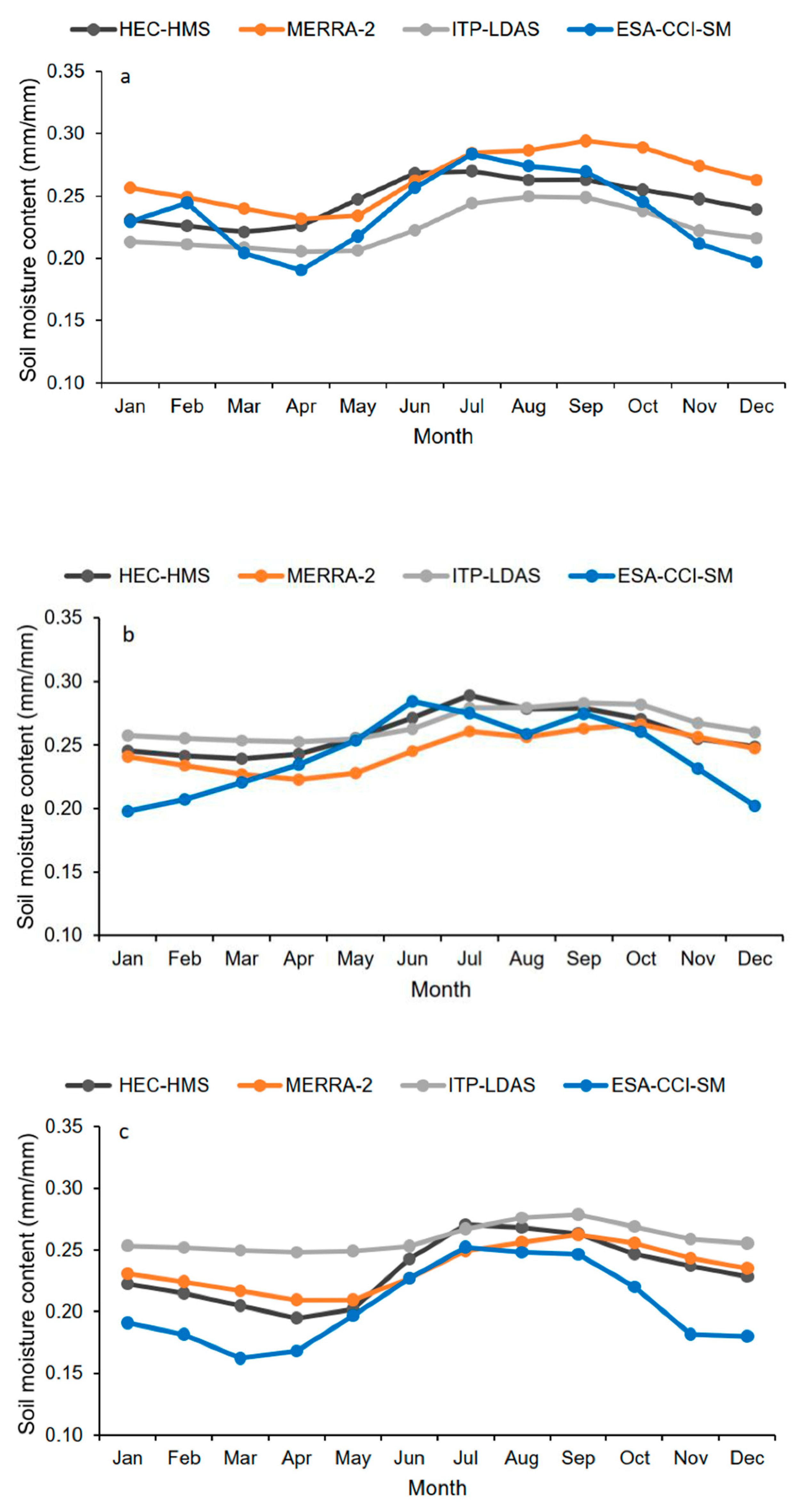
Soil moisture content (SMC) simulated by HEC-HMS was compared with the data obtained from MERRA-2, ITP-LDAS, and ESA-CCI-SM products (described in Table 1) for the period 2001–2010 over the TRHR. On the whole, the R values ranged from 0.44 (ITP-LDAS) to 0.84 (MERRA-2), the RMSE values from 0.015 (MERRA-2) to 0.035 (ITP-LDAS), and the PVD values from −10.2 (ITP-LDAS) to 11.5 (ESA-CCI-MS) in the TRHR (Table 6). In the case of the SLR, the highest correlation and lowest deviation (PVD) were obtained with ESA-CCI-MS, followed by MERRA-2. However, RMSE was the lowest for MERRA-2, followed by ESA-CCI-MS (Table 6). Figure 8a shows that the model’s SMC followed all three datasets well, but overestimated from the ITP-LDAS data in the SLR. In the case of the SYER, the highest R and the lowest RMSE values were calculated with MERRA-2, followed by ESA-CCI-MS. However, PVD values were the lowest for ITP-LDAS, followed by MERRA-2 (Table 6). Figure 8b shows that the model also captured the annual cycle of all three datasets well. In the case of the SYAR, better results were obtained for MERRA-2, followed by ESA-CCI-MS (Table 6). However, the model overestimated ESA-CCI-MS and underestimated IPT-LDAS (Figure 8c). We also compared SMC with previous studies such as Deng, et al. [92], Yuan, et al. [93], Zeng, et al. [94], and Zhang, et al. [95] that have used observed SMC. According to these studies, observed SMC at Maqu and Maduo varies between 0.07 and 0.38 (mm/mm) and 0.01 and 0.18 (mm/mm), respectively, during an annual cycle, with the maximum values in the wet season. Nonetheless, the mean annual values of the present study at Maqu and Maduo were comparable with the observations.

3.2.2. Baseflow

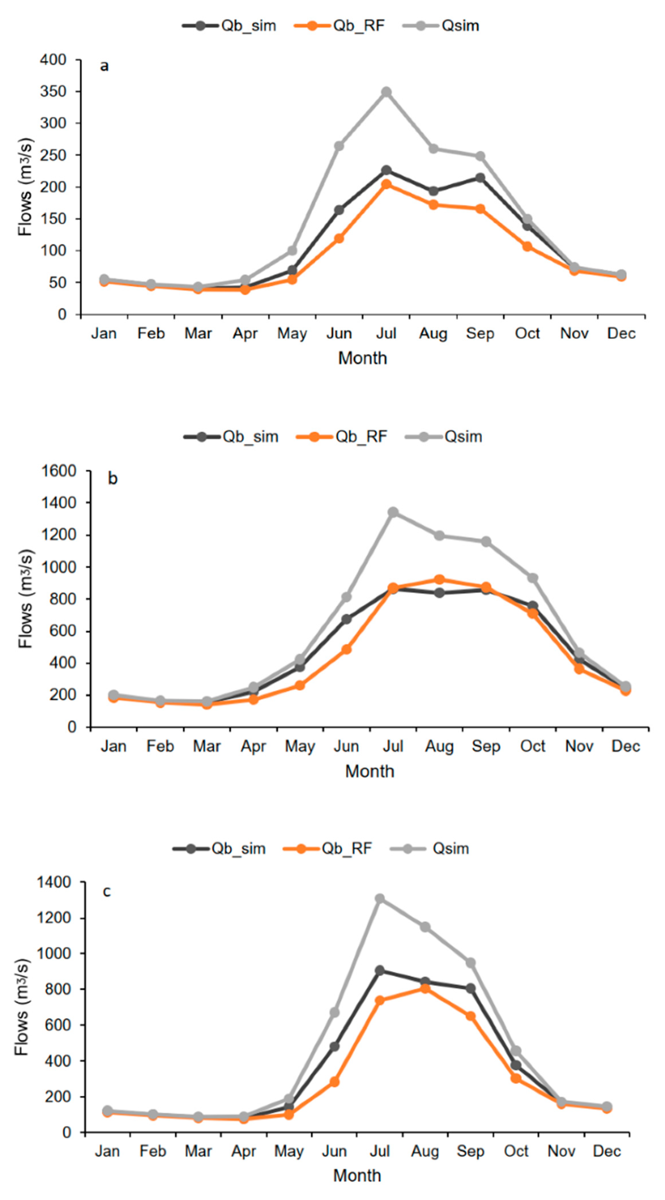
For the evaluation of baseflow simulated by HEC-HMS, we used baseflow separated by the recursive digital filter (RDF) [62] for the period 1981–2015. Table 6 shows that the simulated baseflow has a high correlation (>0.94) with RDF in all three river basins. The values of RMSE were 29 m3/s, 100 m3/s, and 113 m3/s in the SLR, SYER, and SYAR, respectively. PDV was above 15% in the SLR and SYAR and below 10% in the SYER. Figure 9 shows that the model overestimated in all months except in July in the SYER. In the low flow months (November–April), the snowfall period, baseflow must be the same as the streamflow, but baseflow from RDF was lower than the streamflow. Nevertheless, the baseflow simulated by HEC-HMS was almost the same as the streamflow in the low flow months. Therefore, we can conclude that baseflow simulated by HEC-HMS was more rational than RDF. Baseflow simulated by the model contributed 77–78% to streamflow, while RDF contributed 65–73% to streamflow on an annual basis. Some studies, such as Chen, et al. [96], Liu, et al. [97], Lu, et al. [98], and Qian, et al. [99], have simulated or separated baseflow in the TRSR, but all showed different results. Chen, Zheng, Chen and Liu [96] and Qian, Wan, Wang, Lv and Liang [99] determined a baseflow of 65–78% of streamflow using different digital filters in the SYER and SYAR; Liu, Yao, Wang and Yu [97] explored only about 30% of baseflow using Global Land Data Assimilation System (GLDAS) products; and Lu, Wang, Shao, Yu, Hao, Xing, Yong and Li [98] simulated 50–54% of baseflow using the VIC model in the SYAR and SYER. During the recession analysis (Section 2.4.2, we estimated high values of recession constant, confirming baseflow dominance in the region.

3.2.3. Terrestrial Water Storage

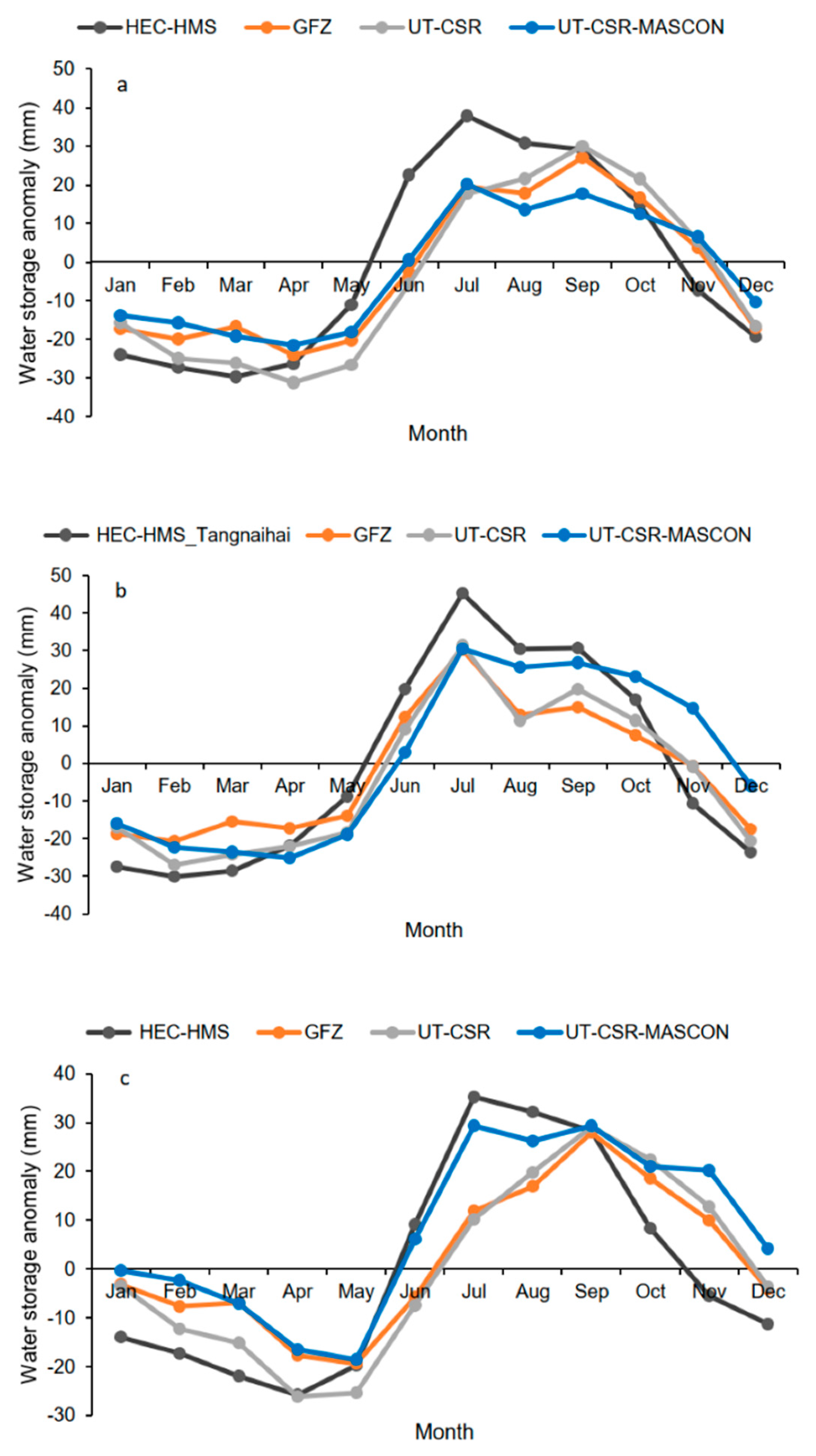
In the present study, terrestrial water storage (HEC-TWS) estimated by HEC-HMS was evaluated with GRACE data, as in Yuan, Ji, Wang, Liang, Yang, Ye, Su and Wen [93]. Since GRACE-TWS is in the form of anomalies relative to the mean of 2004–2009, we also calculated anomalies of HEC-TWS in the region, the same as GRACE. For the evaluation, we used three solutions of GRACE (i.e., GFZ, UT-CSR, and UT-CSR-Mascon) for 2002–2015. The HEC-TWS anomalies had high correlations with three solutions, ranging from 0.70 to 0.76 in the SLR, 0.70 to 0.79 in the SYER, and 0.55 to 0.66 in the SYAR. RMSE ranged between 17 mm and 29 mm in all three basins for three solutions, and PVD ranged between −24% and 35%. According to all three indicators, the HEC-TWS anomalies were best captured by UT-CRS, followed by the GFZ. Figure 10 shows that the annual patterns of GRACE-TWS anomalies were well followed by HEC-TWS in all three headwaters. However, the model underestimated during the dry months (November–March) and overestimated during the wet period, especially in June–August. For the comparison of TWS with the previous studies, we could not find any study simulating TWS using a hydrological model, especially using a conceptual model, for a longer period than GRACE-TWS, except Yuan, Ji, Wang, Liang, Yang, Ye, Su and Wen [93]. They simulated for the period 1979–2014 using a land surface model, but they also validated their results with GRACE-TWS. However, most studies such as Huang, et al. [100], Jing, et al. [101], and Xu, et al. [102] used GRACE-TWS either for the evaluation of Interim Reanalysis Data and GLDAS data or the assessment of other hydrological components such as groundwater and evapotranspiration.

3.2.4. Snow Water Equivalent

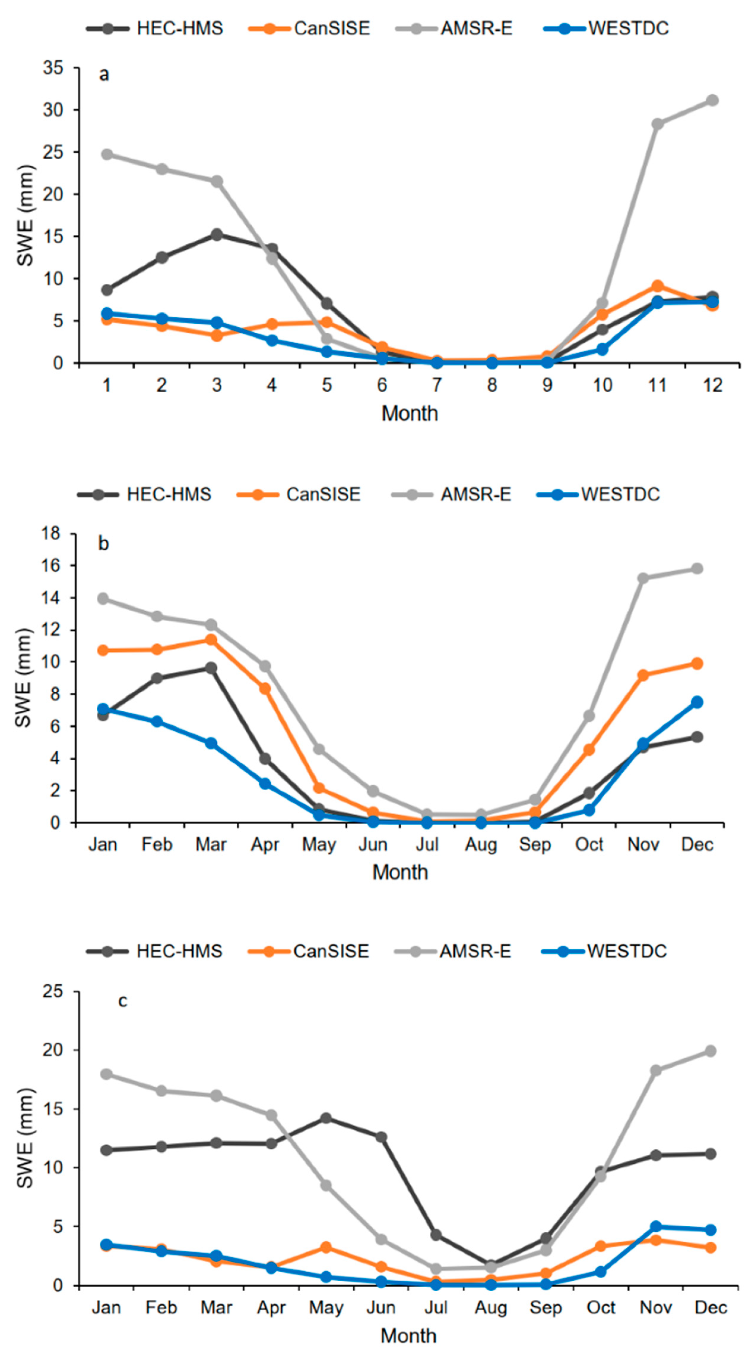
For the evaluation of SWE simulated by HEC-HMS (HEC-SWE), we obtained SWE data from three datasets, i.e., CanSISE, AMSR-E, and WESTDC (Table 1), for the period 2001–2010. The R values ranged from 0.51 (CanSISE) to 0.75 (AMSR-E) in the SLR, from 0.73 (AMRS-E) to 0.82 (CanSISE) in the SYER, and from 0.24 (CanSISE) to 0.33 (AMRS-E) in the SYAR (Table 6). PVD showed that the model underestimated (11–60%) AMSR-E and overestimated (about 22–410%) from CanSISE and WESTDC in all three basins, most of the time. Although correlations were high in the SLR and SYER, PVD and RMSE were also high. Figure 11 clearly shows that the model overestimated from CanSISE and WESTDC but underestimated from AMRS-E in all three basins, except in the SYER, where the model also underestimated from CanSISE. Dai, et al. [103] and Yang, et al. [104] also explored that the estimated SWE by observed snow depth was underestimated by AMRS-E-SWE, especially over grassland areas, in QTP and the Tibetan Plateau, respectively. Significant differences between in situ and remote sensing products have also been reported over the Contiguous United States [105].
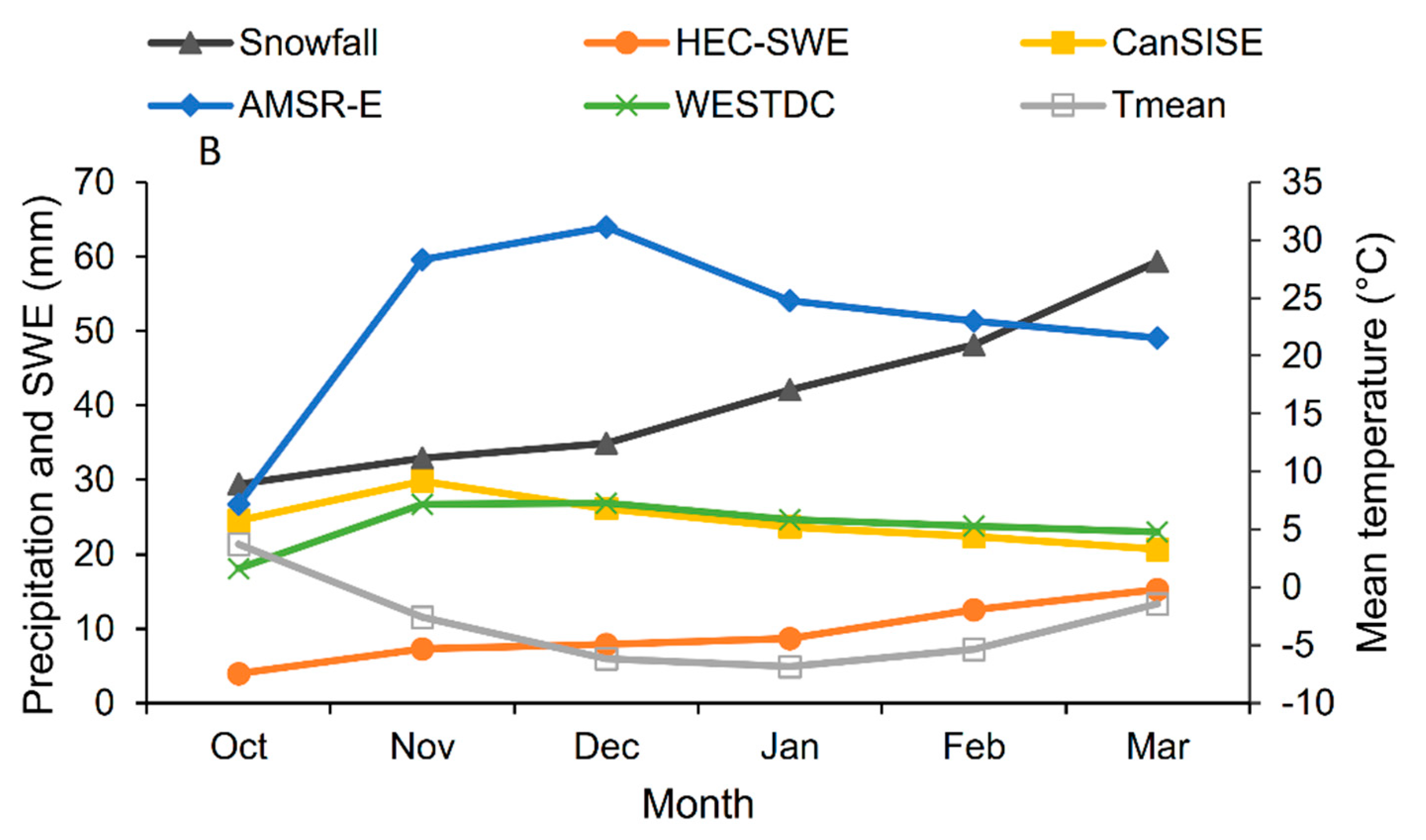
Figure 11 displays that CanSISE and WESTDC were comparable with each other but underestimated from AMSR-E in all three basins. On the whole, we can say that HEC-SWE is not comparable with the remote sensing products, but we cannot say that it is wrong because these products are also not comparable with each other and have some uncertainties. For the evaluation of HEC-SWE, we estimated accumulated snowfall during the snowfall period (October–March) in the SLR and plotted along with remote sensing products and HEC-SWE, as shown in Figure 12. The pattern of HEC-SWE was well in line with the pattern of snowfall in the SLR. For example, HEC-SWE started to accumulate from mid-October and reached a peak in March, very similar to the accumulated snowfall. This indicates that our results are rational because SWE should be maximum in March because the temperature remains below the freezing point from October to March in the SLR (Figure 12). However, the remote sensing products showed peaks for SWE in November or December. Since uncertainties are high in the remote sensing datasets, we need field observations for an accurate evaluation of HEC-SWE.

3.2.5. Actual Evapotranspiration

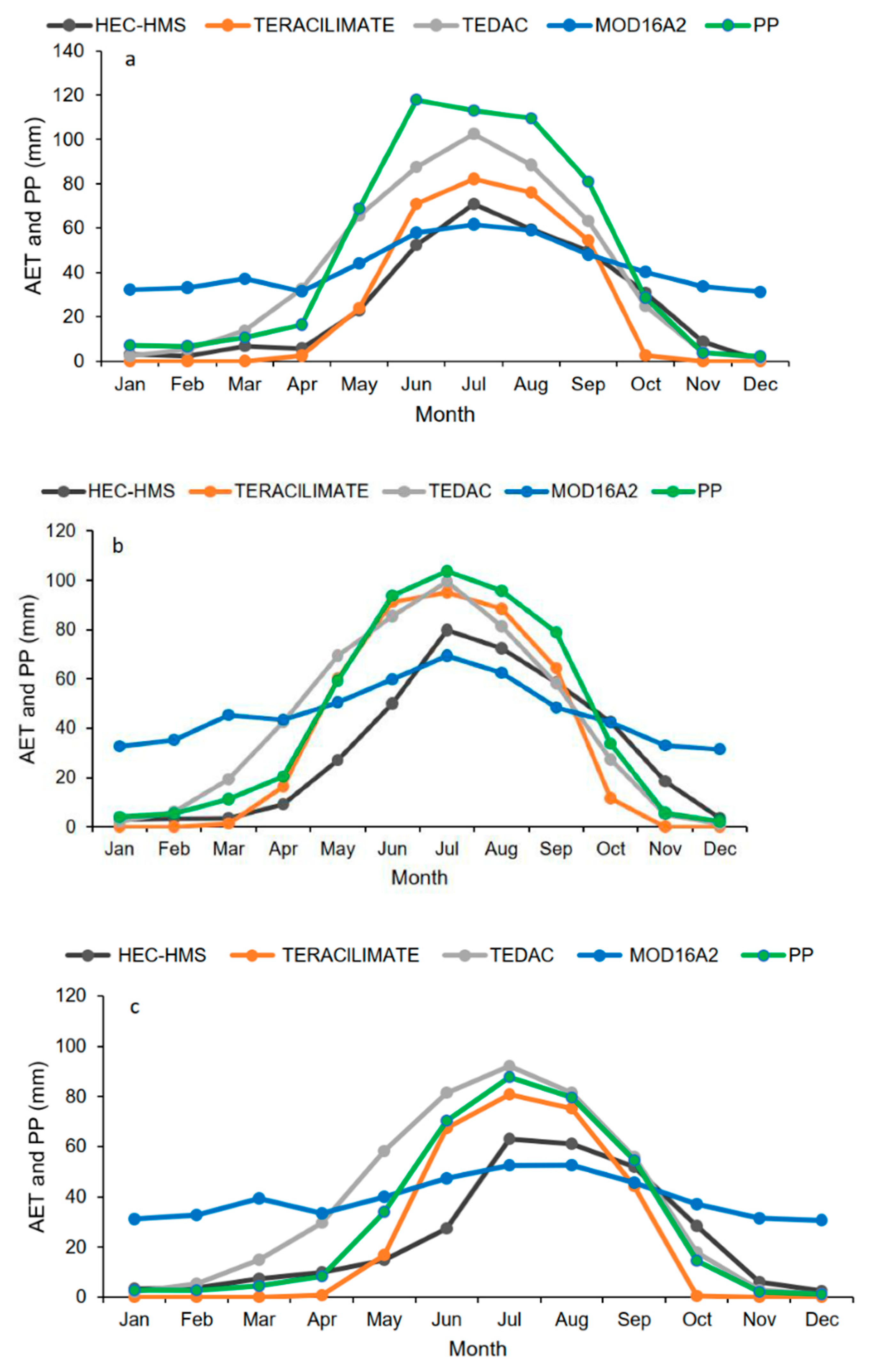
For the evaluation of AET estimated by HEC-HMS (HEC-AET), three products, MOD16A2, TERACLIMATE, and TEDAC, were used from 2000 to 2010. Table 6 shows high correlations with all three products, ranging from 0.73 (MOD16A2) to 0.89 (TERACLIMATE) in all three basins. The highest correlations were found with TERACLIMATE, followed by TEDAC in all three basins. The PVD values were in the satisfactory range for TERACLIMATE in all three basins, ranging from −13.5% to 0.1%. However, the PVD values for MOD16A2 and TEDAC were not satisfactory in all three basins, ranging from −42% to −25%. The PVD values showed that the model underestimated all three products in all three basins, except TERACLIMATE in the SLR.
Figure 13 shows the mean monthly AET estimated by HEC-HMS and three products for the period 2000–2010. The monthly precipitation was also plotted with AETs, which helped to evaluate the estimated AET. The patterns of TERACLIMATE and TEDAC were followed well by HEC-AET in all three basins. However, HEC-AET was underestimated by both products in most months, especially during June–August. MOD16A2 highly overestimated estimated AET during cold and dry months in all three basins, which does not appear rational. We can also evaluate HEC-AET with precipitation for a long period annual mean. It was noted that the mean annual HEC-AET, TERACLIMATE, TEDAC, and MOD16A2 were 60%, 60%, 87%, and 90% of precipitation, respectively, in the SLR; 77%, 79%, 122%, and 131% of precipitation in the SYAR, respectively; and 72%, 83%, 97%, and 108% of precipitation in the SYER, respectively. The AET values of TEDAC and MOD16A2 do not look rational because AET from these products contained a high percentage (>90%) of precipitation. Previous studies such as Li, et al. [106], Sato, et al. [107], Xue, et al. [108], and Zhang, Su, Yang, Hao and Tong [89] have also reported an AET of about 70% of the precipitation, similar to this study, and an even smaller percentage (60% of precipitation) was reported by Bei, et al. [109]. From the above discussion, it can be concluded that HEC-AET and TERACLIMATE appear rational compared to TEDAC and MOD16A2 in the TRHR.

3.3. Uncertainties and Limitations

In general, there are four main sources of uncertainties in hydrological modeling [110], i.e., input data, output data, model structural, and parametric uncertainties. One uncertainty related to data in the region is that the data required to simulate hydrological components are not enough in this region of complex topography. For example, there are only 6–10 climate stations in and around the SYAR (158, 027 km2). This means that the gauge density (about 13,000 km2/gauge) is so sparse compared to the density suggested by the World Meteorological Organization (250–1000 km2/gauge) in similar kinds of harsh conditions [111]. Although reanalysis and remote sensing datasets (RRSD) are suitable alternatives, these also contain uncertainties, as we observed in Section 3.2.4 For example, we observed that SWE data from RRSD products showed large differences from each other (Figure 11). This can be due to the different tools and techniques used in the retrieval of these datasets. Despite all advances in the development of models, they still cannot entirely represent the hydrological system of a region because of a lack of enough understanding of the hydrological cycle. According to [112], the estimation of parameters during the calibration process can be another source of uncertainty in a hydrological model because it is impossible to determine the exact parameters of a study area.
There are also some limitations in HEC-HMS used in the present study. For example, it has only one option (Temperature Index Method to estimate the snowmelt water, which mainly depends on temperature. However, snowmelt is a complex method, which requires a complete energy balance along with the water balance approach. Additionally, some basic parameters such as PX, base temperature, and wet-melt rate in TIM are used for the whole basin. However, these should be used on sub-basin level, even on an elevation-band level in each sub-basin, because these can vary spatially in a region, especially a region having complex mountainous terrain such as the TRHR. In HEC-HMS, instead of precipitation and temperature, the other climatic variables such as wind speed, relative humidity, and sunshine hours are not spatially distributed properly using some sophisticated techniques such as inverse distance weighting or Thiessen Polygon methods. For example, each sub-basin is assigned by only one climate station located in or around the sub-basin.
In this study, we used point-based climate station data, which are very small in number as compared to the area of the region. In addition, the model was calibrated and validated for only streamflow gauges. In the future, we can use gridded satellite climate data such as the Tropical Rainfall Measuring Mission (TRMM). In addition, the model results can be compared with other hydrological model (e.g., SWAT) using the same mythology.

4. Conclusions

In this study, we wanted to configure HEC-HMS so that it could simulate all the important hydrological components (e.g., streamflow, baseflow, soil moisture content, terrestrial water storage, and snowmelt water) in the Three-River Headwater Region (TRHR). However, the main problem is the inefficient built-in auto-calibration methods in HEC-HMS, especially when we include Soil Moisture Accounting (SMA) and Temperature Index Method (TIM). Secondly, no studies have been reported having a comprehensive approach that can be used to configure HEC-HMS in such a way that all the important hydrological components (e.g., streamflow, baseflow, soil moisture content, terrestrial water storage, snowmelt water, and evapotranspiration) can be simulated. Therefore, in this study, we designed a comprehensive approach to configure HEC-HMS so that the model can generate all the important components satisfactorily. The approach was based on providing a systematic way to determine some rational initial values for the process parameters, sensitive parameters, and relations between parameters and hydrograph components (e.g., low flow, peaks, and rising and falling limbs). This will reduce the time of calibration and enhance the deep understanding of the hydrological processes.
The results showed that HEC-HMS has the capability to simulate almost all the important components satisfactorily if we configure the model properly and rationally. This study will be a guideline for the modelers and users of HEC-HMS and similar kinds of other hydrological models.

Supplementary Materials

The following supporting information can be downloaded at: https://www.mdpi.com/article/10.3390/w14182778/s1, Figure S1: Schematic diagram of Temperature Index method in HEC-HMS. PX-temperature discriminates between rain and snow. Cold content (mm w.e.) is calculated based on air temperature and snowpack temperature. Liquid Water Capacity (LWC) is the amount of melted water that stores in the snowpack before liquid water becomes available at the ground surface for runoff or infiltration. Figure S2: Schematic diagram of soil moisture accounting algorithm in HEC-HMS.

Author Contributions

The research work (e.g., conceptualization, methodology, and analysis) was designed and accomplished by the first author R.M. under the supervision of the second author S.J. All authors have read and agreed to the published version of the manuscript.

Funding

This research was funded by Qinghai Provincial Natural Science Foundation (grant number 2019-ZJ-7020) and Scientific Research and Promotion Projects of the Second Phase Project of Ecological Protection and Construction of the Three Rivers Source in Qinghai Province (2018-S-3).

Data Availability Statement

The open-source reanalysis and remote sensing data used in this study are cited in Table 1. Observed streamflow and climatic data were obtained from Hydrology and Water Resources Survey Bureau of Qinghai (HWRSBQ) province and the Qinghai Meteorological Bureau (QMB), respectively, and are available from the corresponding author with the permission of the agencies.

Acknowledgments

We are grateful to the Scientific Research and Promotion Projects of the Second Phase Project of Ecological Protection and Construction of the Three Rivers Source in Qinghai Province (2018-S-3) and Qinghai Provincial Natural Science Foundation (2019-ZJ-7020). Many thanks are offered to the Hydrology and Water Resources Survey Bureau of Qinghai province and the Qinghai Meteorological Bureau for providing discharge and climate data, respectively. Lastly, we offer gratitude to the scientific community for providing remote sensing, land and soil characteristics, reanalysis datasets such as NASA, FAO, National Snow & Ice Data Center, and all others mentioned in the data section.

Conflicts of Interest

The authors declare no conflict of interest. The funders had no role in the design of the study; in the collection, analyses, or interpretation of data; in the writing of the manuscript; or in the decision to publish the results.

References

  1. Edwards, P.J.; Williard, K.W.J.; Schoonover, J.E. Fundamentals of watershed hydrology. J. Contemp. Water Res. Educ. 2015, 154, 3–20. [Google Scholar] [CrossRef]
  2. Wu, P.; Christidis, N.; Stott, P. Anthropogenic impact on Earth’s hydrological cycle. Nat. Clim. Change 2013, 3, 807–810. [Google Scholar] [CrossRef]
  3. Jain, S.K.; Singh, V.P. Hydrological Cycles, Models and Applications to Forecasting. In Handbook of Hydrometeorological Ensemble Forecasting; Duan, Q., Pappenberger, F., Thielen, J., Wood, A., Cloke, H.L., Schaake, J.C., Eds.; Springer: Berlin/Heidelberg, Germany, 2017; pp. 1–28. [Google Scholar]
  4. Pinto, D.B.; Silva, A.M.; Mello, C.R.; Beskow, S.; Coelho, G. Application of the Soil and Water Assessment Tool (SWAT) for sediment transport simulation at a headwater watershed in Minas Gerais State, Brazil. In Proceedings of the International Symposium on Erosion and Landscape Evolution (ISELE), Anchorage, AK, USA, 18–21 September 2011; p. 145. [Google Scholar]
  5. Singh, V.; Mishra, A.; Chowdhary, H.; Khedun, C.P. Climate Change and Its Impact on Water Resources. In Modern Water Resources Engineering; Wang, L.K., Yang, C.T., Eds.; Humana Press: Totowa, NJ, USA, 2014. [Google Scholar]
  6. Miller, M.P.; Susong, D.D.; Shope, C.L.; Heilweil, V.M.; Stolp, B.J. Continuous estimation of baseflow in snowmelt-dominated streams and rivers in the Upper Colorado River Basin: A chemical hydrograph separation approach. Water Resour. Res. 2014, 50, 6986–6999. [Google Scholar] [CrossRef]
  7. Xu, M. Study on water storage change and its consideration in water balance in the mountain regions over arid northwest China. Adv. Meteorol. 2017, 2017, 4291765. [Google Scholar] [CrossRef]
  8. Yan, C.-A.; Zhang, W.; Zhang, Z. Hydrological modeling of the Jiaoyi Watershed (China) using HSPF model. Sci. World J. 2014, 2014, 672360. [Google Scholar] [CrossRef]
  9. Kan, G.; He, X.; Li, J.; Ding, L.; Hong, Y.; Zhang, H.; Liang, K.; Zhang, M. Computer aided numerical methods for hydrological model calibration: An overview and recent development. Arch. Comput. Methods Eng. 2019, 26, 35–59. [Google Scholar] [CrossRef]
  10. Kumarasamy, K.; Belmont, P. Calibration parameter selection and watershed hydrology model evaluation in time and frequency domains. Water 2018, 10, 710. [Google Scholar] [CrossRef]
  11. Yin, Z.; Liao, W.; Lei, X.; Wang, H.; Wang, R. Comparing the Hydrological Responses of Conceptual and Process-Based Models with Varying Rain Gauge Density and Distribution. Sustainability 2018, 10, 3209. [Google Scholar] [CrossRef]
  12. Singh, V.P. Computer Models of Watershed Hydrology; Water Resources Publications: Littleton, CO, USA, 1995; p. 1144. [Google Scholar]
  13. Sorooshian, S.; Hsu, K.-L.; Coppola, E.; Tomassetti, B.; Verdecchia, M.; Visconti, G. Hydrological Modelling and the Water Cycle; Springer: Berlin, Heidelberg, 2008; p. 302. [Google Scholar]
  14. Dariane, A.B.; Javadianzadeh, M.M.; James, L.D. Developing an efficient auto-calibration algorithm for HEC-HMS program. Water Resour. Manag. 2016, 30, 1923–1937. [Google Scholar] [CrossRef]
  15. Duan, Q.; Sorooshian, S.; Gupta, V.K. Optimal use of the SCE-UA global optimization method for calibrating watershed models. J. Hydrol. 1994, 158, 265–284. [Google Scholar] [CrossRef]
  16. Boyle, D.P.; Gupta, H.V.; Sorooshian, S. Toward improved calibration of hydrologic models: Combining the strengths of manual and automatic methods. Water Resour. Res. 2000, 36, 3663–3674. [Google Scholar] [CrossRef]
  17. Ndiritu, J. A comparison of automatic and manual calibration using the Pitman model. Phys. Chem. Earth Parts A/B/C 2009, 34, 729–740. [Google Scholar] [CrossRef]
  18. Bhuiyan, A.K.M.H.; McNairn, H.; Powers, J.; Merzouki, A. Application of HEC-HMS in a cold region watershed and use of radarsat-2 soil moisture in initializing the model. Hydrology 2017, 4, 9. [Google Scholar] [CrossRef]
  19. Gebre, S. Application of the HEC-HMS model for runoff simulation of upper Blue Nile River basin. Hydrol. Curr. Res. 2015, 6, 1000199. [Google Scholar] [CrossRef]
  20. Koch, R.; Bene, K. Continuous hydrologic modeling with HMS in the Aggtelek Karst region. Hydrology 2014, 1, 1–7. [Google Scholar] [CrossRef]
  21. Ouédraogo, A.W.; Raude, M.J.; Gathenya, M.J. Continuous modeling of the Mkurumudzi River catchment in Kenya using the HEC-HMS conceptual model: Calibration, validation, model performance evaluation and sensitivity analysis. Hydrology 2018, 5, 44. [Google Scholar] [CrossRef]
  22. Bashar, K.; Zaki, A.F. SMA based continuous hydrologic simulation of the Blue Nile. In Proceedings of the International Conference of UNESCO Flanders FUST FRIEND/NILE Project “Towards a Better Cooperation”, Sharm El-Sheikh, Egypt, 12–15 November 2005; p. 10. [Google Scholar]
  23. Chea, S.; Oeurng, C. Flow simulation in an ungauged catchment of Tonle Sap Lake Basin in Cambodia: Application of the HEC-HMS model. Water Util. J. 2017, 17, 3–17. [Google Scholar]
  24. Fleming, M.; Neary, V. Continuous hydrologic modeling study with the Hydrologic Modeling System. J. Hydrol. Eng. 2004, 9, 175–183. [Google Scholar] [CrossRef]
  25. Gyawali, R.; David, W.W. Continuous hydrologic modeling of snow-affected watersheds in the Great Lakes Basin using HEC-HMS. J. Hydrol. Eng. 2013, 18, 29–39. [Google Scholar] [CrossRef]
  26. Neary, V.S.; Habib, E.; Fleming, M. Hydrologic modeling with NEXRAD precipitation in Middle Tennessee. J. Hydrol. Eng. 2004, 9, 339–349. [Google Scholar] [CrossRef]
  27. Mahmood, R.; Jia, S.; Lv, A.; Zhu, W. A preliminary assessment of environmental flow in the three rivers’ source region, Qinghai Tibetan Plateau, China and suggestions. Ecol. Eng. 2020, 144, 105709. [Google Scholar] [CrossRef]
  28. Jiang, C.; Zhang, L. Ecosystem change assessment in the Three-river Headwater Region, China: Patterns, causes, and implications. Ecol. Eng. 2016, 93, 24–36. [Google Scholar] [CrossRef]
  29. Jiang, C.; Zhang, L. Climate change and its impact on the eco-environment of the Three-Rivers Headwater Region on the Tibetan Plateau, China. Int. J. Environ. Res. Public Health 2015, 12, 12057. [Google Scholar] [CrossRef]
  30. Shen, X.; An, R.; Feng, L.; Ye, N.; Zhu, L.; Li, M. Vegetation changes in the Three-River Headwaters Region of the Tibetan Plateau of China. Ecol. Indic. 2018, 93, 804–812. [Google Scholar] [CrossRef]
  31. Jarvis, A.; Reuter, H.I.; Nelson, A.; Guevara, E. Hole-Filled Seamless SRTM data V4; International Centre for Tropical Agriculture: Cali, CO, USA, 2008. [Google Scholar]
  32. Loveland, T.R.; Reed, B.C.; Brown, J.F.; Ohlen, D.O.; Zhu, Z.; Yang, L.; Merchant, J.W. Development of a global land cover characteristics database and IGBP DISCover from 1 km AVHRR data. Int. J. Remote Sens. 2000, 21, 1303–1330. [Google Scholar] [CrossRef]
  33. Fischer, G.; Nachtergaele, F.; Prieler, S.; van Velthuizen, H.T.; Verelst, L.; Wiberg, D. Global Agro-ecological Zones Assessment for Agriculture (GAEZ 2008); FAO: Rome, Italy; IIASA: Laxenburg, Austria, 2008. [Google Scholar]
  34. Tedesco, M.; Kelly, R.; Foster, J.L.; Chang, A.T. AMSR-E/Aqua 5-Day L3 Global Snow Water Equivalent EASE-Grids, Version 2; NASA National Snow and Ice Data Center Distributed Active Archive Center: Boulder, CO, USA; Available online: https://nsidc.org/data/ae_5dsno/versions/2 (accessed on 3 September 2019).
  35. Mudryk, L.R.; Derksen, C.; Kushner, P.J.; Brown, R. Characterization of Northern Hemisphere Snow Water Equivalent Datasets, 1981–2010. J. Clim. 2015, 28, 8037–8051. [Google Scholar] [CrossRef]
  36. Liyun, D.A.I.; Tao, C.H.E. Long-Term Series of Daily Snow Depth Dataset in China (1979–2019); National Tibetan Plateau Data Center: Beijing, China, 2015. [Google Scholar] [CrossRef]
  37. Yang, K. The Soil Moisture Dataset of China Based on Microwave Data Assimilation (2002–2011). In The Soil Moisture Dataset of China Based on Microwave Data Assimilation (2002–2011); National Tibetan Plateau Data Center: Beijing, China, 2018. [Google Scholar] [CrossRef]
  38. GMAO. Global Modeling and Assimilation Office (GMAO). MERRA-2 tavgU_2d_lnd_Nx: 2d, diurnal, Time-Averaged, Single-Level, Assimilation, Land Surface Diagnostics V5.12.4; Goddard Earth Sciences Data and Information Services Center (GES DISC): Greenbelt, MD, USA, 2015. [Google Scholar] [CrossRef]
  39. Swenson, S.C. GRACE Monthly Land Water Mass Grids NETCDF RELEASE 5.0. 2012. Available online: https://podaac.jpl.nasa.gov/dataset/TELLUS_LAND_NC_RL05 (accessed on 1 September 2022).
  40. Mao, J.; Yan, B. Global Monthly Mean Leaf Area Index Climatology, 1981–2015; ORNL DAAC: Oak Ridge, TN, USA, 2019. [Google Scholar] [CrossRef]
  41. Abatzoglou, J.T.; Dobrowski, S.Z.; Parks, S.A.; Hegewisch, K.C. TerraClimate, a high-resolution global dataset of monthly climate and climatic water balance from 1958–2015. Sci. Data 2018, 5, 170191. [Google Scholar] [CrossRef] [Green Version]
  42. Jozsef, S.; Yinsheng, Z.; Ning, M.A.; Wenbin, L.I.U. Terrestrial Evapotranspiration Dataset Across China (1982–2017); National Tibetan Plateau Data Center: Beijing, China, 2019. [Google Scholar] [CrossRef]
  43. Running, S.; Mu, Q.; Zhao, M. MOD16A2 MODIS/Terra Net Evapotranspiration 8-Day L4 Global 500m SIN Grid V006; NASA EOSDIS Land Processes DAAC: Sioux Falls, SD, USA, 2017. [Google Scholar] [CrossRef]
  44. William, A.S.; Fleming, M.J. Hydrologic Modeling System HEC-HMS: User’s Manual: Version 3.5; Hydrologic Engineering Center; Institute for Water Resources Davis: Davis, CA, USA, 2010; p. 318. [Google Scholar]
  45. Ramly, S.; Tahir, W. Application of HEC-GeoHMS and HEC-HMS as rainfall–runoff model for flood simulation. In ISFRAM 2015; Springer: Singapore, 2016; pp. 181–192. [Google Scholar]
  46. Munyaneza, O.; Mukubwa, A.; Maskey, S.; Uhlenbrook, S.; Wenninger, J. Assessment of surface water resources availability using catchment modelling and the results of tracer studies in the mesoscale Migina Catchment, Rwanda. Hydrol. Earth Syst. Sci. 2014, 18, 5289–5301. [Google Scholar] [CrossRef]
  47. Mahmood, R.; Jia, S. Assessment of impacts of climate change on the water resources of the transboundary Jhelum River basin of Pakistan and India. Water 2016, 8, 246. [Google Scholar] [CrossRef]
  48. Rangari, V.A.; Sridhar, V.; Umamahesh, N.V.; Patel, A.K. Rainfall runoff modelling of urban area using HEC-HMS: A case study of Hyderabad city. In Advances in Water Resources Engineering and Management; Springer: Singapore, 2020; pp. 113–125. [Google Scholar]
  49. Halwatura, D.; Najim, M.M.M. Application of the HEC-HMS model for runoff simulation in a tropical catchment. Environ. Model. Softw. 2013, 46, 155–162. [Google Scholar] [CrossRef]
  50. Meenu, R.; Rehana, S.; Mujumdar, P.P. Assessment of hydrologic impacts of climate change in Tunga-Bhadra River basin, India with HEC-HMS and SDSM. Hydrol. Processes 2013, 27, 1572–1589. [Google Scholar] [CrossRef]
  51. Hou, Z.-W.; Qin, C.-Z.; Zhu, A.X.; Liang, P.; Wang, Y.-J.; Zhu, Y.-Q. From manual to intelligent: A review of input data preparation methods for geographic modeling. Int. J. Geo-Inf. 2019, 8, 376. [Google Scholar] [CrossRef]
  52. Zhang, Q.; Zhou, A.; Jin, Y. RM-MEDA: A regularity model-based multi-objective estimation of distribution algorithm. IEEE Trans. Evol. Comput. 2008, 12, 41–63. [Google Scholar] [CrossRef]
  53. Nasiri, S.; Ansari, H.; Ziaei, A.N. Simulation of water balance equation components using SWAT model in Samalqan Watershed (Iran). Arab. J. Geosci. 2020, 13, 421. [Google Scholar] [CrossRef]
  54. Ahbari, A.; Stour, L.; Agoumi, A.; Serhir, N. Estimation of initial values of the HMS model parameters: Application to the basin of Bin El Ouidane (Azilal, Morocco). J. Mater. Environ. Sci. 2018, 9, 305–317. [Google Scholar] [CrossRef]
  55. Cosby, B.J.; Hornberger, G.M.; Clapp, R.B.; Ginn, T.R. A statistical exploration of the relationships of soil moisture characteristics to the physical properties of soils. Water Resour. Res. 1984, 20, 682–690. [Google Scholar] [CrossRef]
  56. Clapp, R.B.; Hornberger, G.M. Empirical equations for some soil hydraulic properties. Water Resour. Res. 1978, 14, 601–604. [Google Scholar] [CrossRef]
  57. Rawls, W.J.; Brakensiek, D.L.; Saxtonn, K.E. Estimation of soil water properties. Trans. ASAE 1982, 25, 1316–1320. [Google Scholar] [CrossRef]
  58. Saxton, K.E.; Rawls, W.J. Soil water characteristic estimates by texture and organic matter for hydrologic solutions. Soil Sci. Soc. Am. J. 2006, 70, 1569–1578. [Google Scholar] [CrossRef]
  59. FAO. In Irrigation Water Management: Irrigation Methods; Training Manual No 5; The International Institute for Land Reclamation and Improvement: Wageningen, The Netherlands, 1988.
  60. Samady, M.K. Continuous Hydrologic Modeling for Analyzing the Effects of Drought on the Lower Colorado River in Texas. Ph.D. Thesis, Michigan Technological University, Houghton, MI, USA, 2017. [Google Scholar]
  61. Raghunath, H.M. Hydrology: Principles, Analysis and Design; New Age International (P) Limited: New Delhi, India, 2006; p. 476. [Google Scholar]
  62. Nathan, R.J.; McMahon, T.A. Evaluation of automated techniques for base flow and recession analyses. Water Resour. Res. 1990, 26, 1465–1473. [Google Scholar] [CrossRef]
  63. Berhail, S.; Ouerdachi, L.; Boutaghane, H. The use of the recession index as indicator for components of flow. Energy Procedia 2012, 18, 741–750. [Google Scholar] [CrossRef]
  64. Brown de Colstoun, E.C.; Huang, C.; Wang, P.; Tilton, J.C.; Tan, B.; Phillips, J.; Niemczura, S.; Ling, P.Y.; Wolfe, R.E. Global Man-made Impervious Surface (GMIS) Dataset from Landsat; NASA Socioeconomic Data and Applications Center (SEDAC): Palisades, NY, USA, 2017. [Google Scholar]
  65. Zhang, X.; Liu, L.; Wu, C.; Chen, X.; Gao, Y.; Xie, S.; Zhang, B. Development of a global 30 m impervious surface map using multisource and multitemporal remote sensing datasets with the Google Earth Engine platform. Earth Syst. Sci. Data 2020, 12, 1625–1648. [Google Scholar] [CrossRef]
  66. Verbeiren, B.; Ho, K.; Wirion, C.; Batelaan, O. An Earth observation based method to assess the influence of seasonal dynamics of canopy interception storage on the urban water balance. Belgeo 2016, 2, 17806. [Google Scholar] [CrossRef]
  67. Cronshey, R.G.; Roberts, R.T.; Miller, N. Urban Hydrology for Small Watersheds; United States Department of Agriculture: Washington, DC, USA, 1986; p. 164. [Google Scholar]
  68. Feldman, A.D. Techinical Reference Manual; Institute for Water Resources: Davis, CA, USA, 2000; p. 157. [Google Scholar]
  69. Clark, C.O. Storage and the unit yydrograph. Trans. Am. Soc. Civ. Eng. 1945, 110, 1419–1446. [Google Scholar] [CrossRef]
  70. USACE. Engineering and Design: Flood-Runoff Analysis (Engineer Manual 1110-2-1417); Military Bookshop; U.S. Army Corps of Engineers: Washington, DC, USA, 1994; p. 228. [Google Scholar]
  71. Devak, M.; Dhanya, C.T. Sensitivity analysis of hydrological models: Review and way forward. J. Water Clim. Change 2017, 8, 557–575. [Google Scholar] [CrossRef] [Green Version]
  72. Haan, C.T. Statistical Methods in Hydrology, 2nd ed.; Wiley-Blackwell; Iowa State Univ. Press: Ames, IA, USA, 2002. [Google Scholar]
  73. García, A.; Sainz, A.; Revilla, J.A.; Álvarez, C.; Juanes, J.A.; Puente, A. Surface water resources assessment in scarcely gauged basins in the north of Spain. J. Hydrol. 2008, 356, 312–326. [Google Scholar] [CrossRef]
  74. Mahmood, R.; Jia, S.; Babel, S.M. Potential Impacts of Climate Change on Water Resources in the Kunhar River Basin, Pakistan. Water 2016, 8, 23. [Google Scholar] [CrossRef]
  75. Verma, A.; Jha, M.; Mahana, R. Evaluation of HEC-HMS and WEPP for simulating watershed runoff using remote sensing and geographical information system. Paddy Water Env. 2010, 8, 131–144. [Google Scholar] [CrossRef]
  76. Murphy, R.; Graszkiewicz, Z.; Hill, P.; Neal, B.; Nathan, R.; Ladson, T. Australian Rainfall and Runoff Revision Project 7: Baseflow for Catchment Simulation; Engineering House: Barton, Australia, P7/S1/004; 2009; p. 121. [Google Scholar]
  77. Brodie, H.K.; Hostetler, S. A review of techniques for analysing baseflow from stream. In Proceedings of the NZHS-IAH-NZSSS 2005 Conference, Auckland, New Zealand, 2 December 2005; p. 2005. [Google Scholar]
  78. Chen, Z.; Jiang, W.; Wu, J.; Chen, K.; Deng, Y.; Jia, K.; Mo, X. Detection of the spatial patterns of water storage variation over China in recent 70 years. Sci. Rep. 2017, 7, 6423. [Google Scholar] [CrossRef]
  79. Ochoa-Sánchez, A.; Crespo, P.; Carrillo-Rojas, G.; Sucozhañay, A.; Célleri, R. Actual evapotranspiration in the high Andean grasslands: A comparison of measurement and estimation methods. Front. Earth Sci. 2019, 7, 55. [Google Scholar] [CrossRef]
  80. Jian, D.; Li, X.; Sun, H.; Tao, H.; Jiang, T.; Su, B.; Hartmann, H. Estimation of actual evapotranspiration by the complementary theory-based advection–aridity model in the Tarim River basin, China. J. Hydrometeorol. 2018, 19, 289–303. [Google Scholar] [CrossRef]
  81. Salama, M.A.; Yousef, K.M.; Mostafa, A.Z. Simple equation for estimating actual evapotranspiration using heat units for wheat in arid regions. J. Radiat. Res. Appl. Sci. 2015, 8, 418–427. [Google Scholar] [CrossRef]
  82. Zhu, W.; Jia, S.; Lall, U.; Cao, Q.; Mahmood, R. Relative contribution of climate variability and human activities on the water loss of the Chari/Logone River discharge into Lake Chad: A conceptual and statistical approach. J. Hydrol. 2019, 569, 519–531. [Google Scholar] [CrossRef]
  83. Van Liew, M.W.; Garbrecht, J. Hydrologic simulation of the little Washita River experimental watershed using SWAT. J. Am. Water Resour. As. 2003, 39, 413–426. [Google Scholar] [CrossRef]
  84. Meng, F.; Su, F.; Yang, D.; Tong, K.; Hao, Z. Impacts of recent climate change on the hydrology in the source region of the Yellow River basin. J. Hydrol. Reg. Stud. 2016, 6, 66–81. [Google Scholar] [CrossRef] [Green Version]
  85. Yang, T.; Wang, X.; Yu, Z.; Krysanova, V.; Chen, X.; Schwartz, F.W.; Sudicky, E.A. Climate change and probabilistic scenario of streamflow extremes in an alpine region. J. Geophys. Res. Atmos. 2014, 119, 8535–8551. [Google Scholar] [CrossRef]
  86. Zhang, Y.; Su, F.; Hao, Z.; Xu, C.; Yu, Z.; Wang, L.; Tong, K. Impact of projected climate change on the hydrology in the headwaters of the Yellow River basin. Hydrol. Processes 2015, 29, 4379–4397. [Google Scholar] [CrossRef]
  87. Guo, M.; Li, J.; Wang, Y.; Bai, P.; Wang, J. Distinguishing the relative contribution of environmental factors to runoff change in the headwaters of the Yangtze River. Water 2019, 11, 1432. [Google Scholar] [CrossRef]
  88. Wang, J.; Luo, S.; Li, Z.; Wang, S.; Li, Z. The freeze/thaw process and the surface energy budget of the seasonally frozen ground in the source region of the Yellow River. Theor. Appl. Climatol. 2019, 138, 1631–1646. [Google Scholar] [CrossRef]
  89. Zhang, L.; Su, F.; Yang, D.; Hao, Z.; Tong, K. Discharge regime and simulation for the upstream of major rivers over Tibetan Plateau. J. Geophys. Res. Atmos. 2013, 118, 8500–8518. [Google Scholar] [CrossRef]
  90. Lauri, H.; Räsänen, T.A.; Kummu, M. Using reanalysis and remotely sensed temperature and precipitation data for hydrological modeling in monsoon climate: Mekong River case study. J. Hydrometeorol. 2014, 15, 1532–1545. [Google Scholar] [CrossRef]
  91. Su, F.; Hong, Y.; Lettenmaier, D.P. Evaluation of TRMM Multisatellite Precipitation Analysis (TMPA) and its utility in hydrologic prediction in the La Plata basin. J. Hydrometeor. 2008, 9, 622–640. [Google Scholar] [CrossRef]
  92. Deng, M.; Meng, X.; Li, Z.; Lyv, Y.; Lei, H.; Zhao, L.; Zhao, S.; Ge, J.; Jing, H. Responses of soil moisture to regional climate change over the Three River Source Region on the Tibetan Plateau. Int. J. Climatol. 2019, 40, 6341. [Google Scholar] [CrossRef]
  93. Yuan, X.; Ji, P.; Wang, L.; Liang, X.Z.; Yang, K.; Ye, A.; Su, Z.; Wen, J. High-Resolution Land Surface Modeling of Hydrological Changes Over the Sanjiangyuan Region in the Eastern Tibetan Plateau: 1. Model Development and Evaluation. J. Adv. Modeling Earth Syst. 2018, 10, 2806–2828. [Google Scholar] [CrossRef]
  94. Zeng, J.; Li, Z.; Quan, C.; Bi, H.; Qiu, J.; Zou, P. Evaluation of remotely sensed and reanalysis soil moisture products over the Tibetan Plateau using in-situ observations. Remote Sens. Environ. 2015, 163, 91–110. [Google Scholar] [CrossRef]
  95. Zhang, Q.; Fan, K.; Singh, V.P.; Sun, P.; Shi, P. Evaluation of Remotely Sensed and Reanalysis Soil Moisture Against In Situ Observations on the Himalayan-Tibetan Plateau. J. Geophys. Res. 2018, 123, 7132–7148. [Google Scholar] [CrossRef]
  96. Chen, L.; Zheng, H.; Chen, Y.D.; Liu, C. Baseflow separation in the source region of the Yellow River. J. Hydrol. Eng. 2008, 13, 541–548. [Google Scholar] [CrossRef]
  97. Liu, Z.; Yao, Z.; Wang, R.; Yu, G. Estimation of the Qinghai-Tibetan Plateau runoff and its contribution to large Asian rivers. Sci. Total Environ. 2020, 749, 141570. [Google Scholar] [CrossRef]
  98. Lu, W.; Wang, W.; Shao, Q.; Yu, Z.; Hao, Z.; Xing, W.; Yong, B.; Li, J. Hydrological projections of future climate change over the source region of Yellow River and Yangtze River in the Tibetan Plateau: A comprehensive assessment by coupling RegCM4 and VIC model. Hydrol. Processes 2018, 32, 2096–2117. [Google Scholar] [CrossRef]
  99. Qian, K.; Wan, L.; Wang, X.-S.; Lv, J.; Liang, S. Periodical characteristics of baseflow in the source region of the Yangtze River. J. Arid. Land 2012, 4, 113–122. [Google Scholar] [CrossRef]
  100. Huang, Y.; Salama, M.; Krol, M.; Velde, R.; Hoekstra, A.; Zhou, Y.; Su, Z. Analysis of long-term terrestrial water storage variations in Yangtze River basin. Hydrol. Earth Syst. Sci. Discuss. 2012, 9, 11487–11520. [Google Scholar] [CrossRef]
  101. Jing, W.; Zhang, P.; Zhao, X. A comparison of different GRACE solutions in terrestrial water storage trend estimation over Tibetan Plateau. Sci. Rep. 2019, 9, 1765. [Google Scholar] [CrossRef]
  102. Xu, M.; Kang, S.; Chen, X.; Wu, H.; Wang, X.; Su, Z. Detection of hydrological variations and their impacts on vegetation from multiple satellite observations in the Three-River Source Region of the Tibetan Plateau. Sci. Total Environ. 2018, 639, 1220–1232. [Google Scholar] [CrossRef]
  103. Dai, L.; Che, T.; Ding, Y.; Hao, X. Evaluation of snow cover and snow depth on the Qinghai–Tibetan Plateau derived from passive microwave remote sensing. Cryosphere 2017, 11, 1933–1948. [Google Scholar] [CrossRef]
  104. Yang, J.; Jiang, L.; Menard, C.; Luojus, K.; Lemmetyinen, J.; Pulliainen, J. Evaluation of snow products over the Tibetan Plateau. Hydrol. Processes 2015, 29, 10427. [Google Scholar] [CrossRef]
  105. Dawson, N.; Broxton, P.; Zeng, X. Evaluation of remotely-sensed snow water equivalent and snow cover extent over the contiguous United States. J. Hydrometeorol. 2018, 19, 1777–1791. [Google Scholar] [CrossRef]
  106. Li, X.; Long, D.; Han, Z.; Scanlon, B.R.; Sun, Z.; Han, P.; Hou, A. Evapotranspiration estimation for Tibetan Plateau headwaters using conjoint terrestrial and atmospheric water balances and multisource remote sensing. Water Resour. Res. 2019, 55, 8608–8630. [Google Scholar] [CrossRef]
  107. Sato, Y.; Ma, X.; Xu, J.; Matsuoka, M.; Zheng, H.; Liu, C.; Fukushima, Y. Analysis of long-term water balance in the source area of the Yellow River basin. Hydrol. Processes 2008, 22, 1618–1629. [Google Scholar] [CrossRef]
  108. Xue, B.-L.; Wang, L.; Li, X.; Yang, K.; Chen, D.; Sun, L. Evaluation of evapotranspiration estimates for two river basins on the Tibetan Plateau by a water balance method. J. Hydrol. 2013, 492, 290–297. [Google Scholar] [CrossRef]
  109. Bei, X.; Yao, Y.; Zhang, L.; Xu, T.; Jia, K.; Zhang, X.; Shang, K.; Xu, J.; Chen, X. Long-Term Spatiotemporal Dynamics of Terrestrial Biophysical Variables in the Three-River Headwaters Region of China from Satellite and Meteorological Datasets. Remote Sens. 2019, 11, 1633. [Google Scholar] [CrossRef]
  110. Renard, B.; Kavetski, D.; Kuczera, G.; Thyer, M.; Franks, S.W. Understanding predictive uncertainty in hydrologic modeling: The challenge of identifying input and structural errors. Water Resour. Res. 2010, 46, 1–22. [Google Scholar] [CrossRef]
  111. Liang, S.; Li, X.; Wang, J. Chapter 17-Precipitation. In Advanced Remote Sensing; Academic Press: Boston, MA, USA, 2012; pp. 533–556. [Google Scholar]
  112. Zhang, J.L.; Li, Y.P.; Huang, G.H.; Wang, C.X.; Cheng, G.H. Evaluation of uncertainties in input data and parameters of a hydrological model using a Bayesian framework: A case study of a snowmelt–precipitation-driven watershed. J. Hydrometeorol. 2016, 17, 2333–2350. [Google Scholar] [CrossRef]
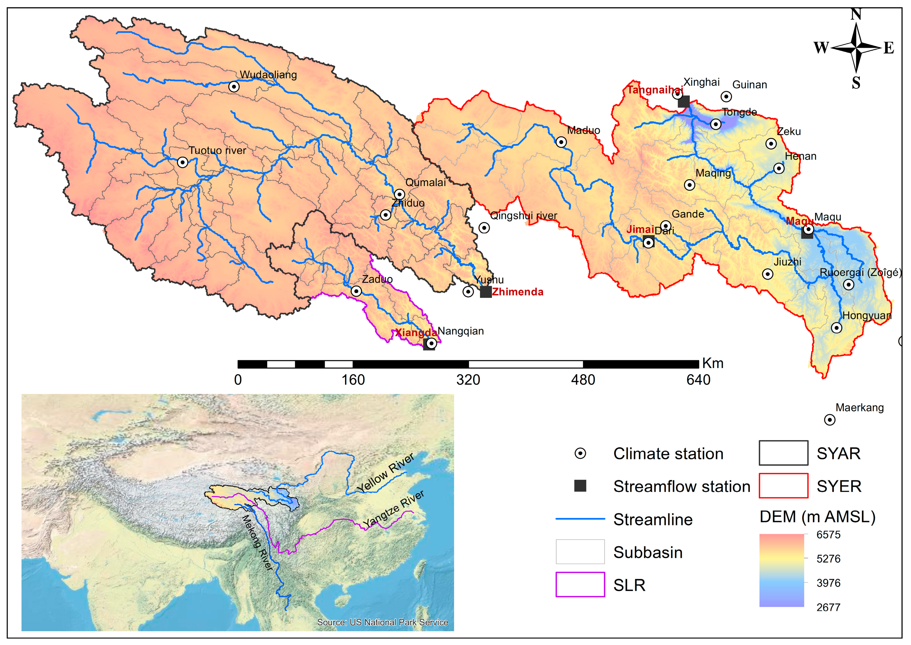
Figure 1. Location map of the Three-River Headwater Region showing streamflow gauges, meteorological stations, and elevation. SYER, source region of the Yellow River; SYAR, source region of the Yangtze River; SLR, source region of the Lancang River.
Water 14 02778 g001
Figure 2. The whole procedure in the development of the hydrological model (HEC-HMS).
Water 14 02778 g002
Figure 3. Some physical characteristics obtained by watershed delineation in the SYER: sub-basin area (km2, red values), sub-basin stream length (km, black values), and slope.
Water 14 02778 g003
Figure 5. Changes in peak and volume with respect to the changes in parameters.
Water 14 02778 g005
Figure 6. The effects of hydrological parameters on the components (e.g., falling limb, rising limb, peak flow, and low flow) of streamflow hydrograph. Black line shows the initial streamflow and gray line shows the streamflow after changing a parameter by 10%. For example, the top-left figure shows that when we increase the max. infiltration, the peak flow component lowers. Similarly, when we increase soil storage (top-middle figure), peak flow lowers and falling limb moves forward.
Water 14 02778 g006
Figure 7. Comparison of observed and simulated streamflow at (a) Jimai station on the Yellow River, (b) Maqu station on the Yellow River, (c) Tangnaihai station on the Yellow River, (d) Zhimenda on the Yangtze River, and (e) Xiangda on the Lancang River hydrometric stations.
Water 14 02778 g007aWater 14 02778 g007bWater 14 02778 g007c
Figure 8. Comparison of soil moisture content simulated by HEC-HMS with ESA-CCI, MERRA-2, and ITP-LDAS data in (a) the SLR, (b) SYER, and (c) SYAR.
Water 14 02778 g008
Figure 9. Comparison of baseflow simulated by HEC-HMS and the recursive digital filter (RDF) in (a) the SLR at Xiangda, (b) SYER at Tangnaihai, and (c) SYAR at Zhimenda. Qb_sim and Qsim are simulated baseflow and streamflow by HEC-HMS, and Qb_RF is the estimated baseflow by the RDF.
Water 14 02778 g009
Figure 10. Comparison of water storage anomalies with the GRACE data in (a) the SLR, (b) SYER, and (c) SYAR, for the period 2002–2015.
Water 14 02778 g010
Figure 11. Comparison of SWE simulated by HEC-HMS with CanSISE, AMSR-E, and WESTDC data in (a) the SLR, (b) SYER, and (c) SYAR.
Water 14 02778 g011
Figure 12. Comparison of remote sensing SWE and HEC-SWE with accumulated snowfall for the period 2001–2010, during the snowfall period (October–March) in the SLR.
Water 14 02778 g012
Figure 13. Comparison of AET with TERACLIMATE, TEDAC, and MOD16A2 data in (a) the SLR, (b) SYER, and (c) SYAR.
Water 14 02778 g013
Table 1. Spatial and temporal data used in the present study.
SRData TypeSpatial/Temporal ResolutionSourceAvailability
1Streamflow dataDailyHydrology and Water Resources Survey Bureau of Qinghai province1980–2015
2Climate dataDailyQinghai Meteorological Bureau (QMB)1980–2015
3DEM90 mNASA’s Shuttle Radar Topography Mission (SRTM), Version 004 [31] (http://srtm.csi.cgiar.org) (accessed on 20 August 2019).Updated 2008
4Land Use Land Cover1 kmGlobal Land Cover Characteristics [32] (https://earthexplorer.usgs.gov/) (accessed on 20 August 2019). 1993
5Soil characteristics1 kmHarmonized World Soil Database Version 1.2 (http://www.fao.org/soils-portal/) (accessed on 20 August 2019) [33]Update 2013
6Snow Water Equivalent (SWE)/snow depth25 km/daily, monthlyAdvanced Microwave Scanning Radiometer-Earth Observing System (AMSR-E), Version 2 [34]2002/6–2011/10
1°/dailyCanadian Sea Ice and Snow Evolution (CanSISE) [35]1981–2010
0.25°/dailyEnvironmental and Ecological Science Data Center for West China (WESTDC) [36]1979–2019
7Soil Moisture Content0.25°/dailyEuropean Space Agency (ESA) Climate Change Initiative Soil Moisture product (ESA-CCI-SM_v4.7), 1978–2019
0.25°/dailyChina Soil Moisture Dataset from Microwave Data Assimilation (ITP-LDAS) [37]2002–2011
0.5°′0.625°/diurnalModern-Era Retrospective analysis for Research and Applications (MERRA-2) [38]1980–2020
8GRACE data300 km/monthlyGeo-forschungs-Zentrum Potsdam (GFZP), University of Texas-Center for Space Research (UT-CSR), and UT-CSR Mascons [39], 2002–2020
9Leaf Area Index0.25°/monthlyGlobal Monthly Mean Leaf Area Index Climatology, 1981–2015 [40]1981–2015
10Evapotranspiration4 km/monthlyTERRACLIMATE [41]1958–2019
0.1°/monthlyTerrestrial evapotranspiration dataset across China, version 1.5 [42]1982–2017
500 m/8-dailyMOD16A2 Version 6 [43]2000–2020
Table 3. Maximum canopy storage in the headwater of the Yellow River, described in Ahbari et al. (2018), Samady (2017), and Verbeiren et al. (2016).
CodeDescription% of the Total AreaCanopy Storage (mm)
1Urban and Built-Up Land0.000.5
2Dryland Cropland and Pasture0.471.5
5Cropland/Grassland Mosaic0.012.0
6Cropland/Woodland Mosaic0.022.0
7Grassland88.612.0
8Shrubland1.992.5
9Mixed Shrubland/Grassland1.662.2
10Savanna1.052.0
11Deciduous Broadleaf Forest0.153.0
12Deciduous Needleleaf Forest0.132.0
14Evergreen Needleleaf Forest0.012.0
15Mixed Forest0.813.0
16Water Bodies1.510.0
17Herbaceous Wetland0.021.0
18Wooded Wetland0.001.0
19Glacier0.120.0
21Wooded Tundra3.432.0
Table 4. Maximum surface storage according to percent slope [24].
SurfaceSlope (%)Max Surface Storage (mm)
Paved impervious areaNA3.2–6.6
Steep, smooth slopes>301.0
Moderate to gentle slopes5–3012.7–6.4
Flat, furrowed land0–550.8
Table 5. Performance evaluation of HEC-HMS in the TRHR on a daily basis.
JimaiMaquTangnaihaiZhimendaXiangda
Calibration
E0.660.850.830.740.69
R20.730.880.890.830.73
PVD (%)4.453.606.248.96−4.29
NRMSE0.460.300.300.510.43
Validation-1
E0.690.830.900.770.74
R20.770.830.900.820.78
PVD12.83.29−1.328.686.66
NRMSE0.390.350.270.490.49
Validation-2
E0.620.820.820.790.61
R20.710.820.820.810.65
PVD21.07−4.38−0.781.36−1.13
NRMSE0.520.420.400.480.55
Table 6. Evaluation of HEC-HMS using different hydrologic components in the TRHR.
Soil Moisture ContentSnow Water EquivalentBaseflowTerrestrial Water Storage ChangesActual Evapotranspiration
ESA-CCI-SMMERRA-2ITP-LDASCanSISEAMSR-E WESTDCDRFGFZUT-CSRUT-CSR_MASCONTERRACLIMATEMOD16A2TEDAC
Analysis Period 2001–20102001–20101981–20152002–20152000–2010
The Source of the Lancang River (SLR)
R0.720.600.440.510.750.720.950.720.700.760.890.790.87
RMSE0.0310.0270.0336.512.56.029.020.022.117.515.323.924.3
PVD (%)4.5−6.69.064.1−51.7111.818.111.0−5.334.30.1−38.6−36.3
The Source of the Yellow River (SYER)
R0.720.740.560.820.730.810.960.700.750.790.850.800.83
RMSE0.0290.0200.0223.66.32.5100.821.720.417.721.924.522.2
PVD (%)6.75.7−2.4−38.4−59.822.47.417.49.118.6−13.5−33.2−25.4
The Source of the Yangtze River (SYAR)
R0.800.840.490.240.330.320.960.640.660.550.860.730.81
RMSE0.0340.0150.0359.78.29.9113.219.219.228.717.323.624.6
PVD (%)11.5−0.9−10.2318.4−11.3410.420.116.35.1−23.8−3.5−42.2−37.6
Publisher’s Note: MDPI stays neutral with regard to jurisdictional claims in published maps and institutional affiliations.