Article

A Data-Driven Dam Deformation Forecasting and Interpretation Method Using the Measured Prototypical Temperature Data

1
College of Geosciences and Engineering, North China University of Water Resources and Electric Power, Zhengzhou 450001, China
2
College of the Built Environment, The University of New South Wales, Sydney, NSW 1001, Australia
*
Author to whom correspondence should be addressed.
Water 2022, 14(16), 2538; https://doi.org/10.3390/w14162538
Submission received: 15 July 2022 / Revised: 10 August 2022 / Accepted: 12 August 2022 / Published: 18 August 2022
(This article belongs to the Special Issue Safety Monitoring and Management of Reservoir and Dams)

Abstract

:
Dam deformation is an intuitive and reliable monitoring indicator for dam structural response. With the increase in the service life of the project, the structural response and environmental quantity data collected by the structural health monitoring (SHM) system show a geometric growth trend. The traditional hydraulic-seasonal-time (HST) model shows poor performance in dealing with massive monitoring data due to the multidimensional data collinearity problem and the inaccurate temperature field simulations. To address these problems, this study proposes a data-driven dam deformation monitoring model for dealing with massive monitoring data based on the light gradient boosting tree (LGB) and Bayesian optimization (BO) algorithm. The proposed BO–LGB method can mine the underlying relationship between temperature changes and dam deformation instead of simple harmonic functions. Moreover, LGB is used to simulate the relationship between high-dimensional environmental quantity data and dam displacement changes, and the BO algorithm is used to determine the optimal hyperparameter selection of LGB based on massive monitoring data. A concrete dam in long-term service was used as the case study, and three typical dam displacement monitoring points were used for model training and validation. The experimental results have indicated that the method can properly consider the collinearity in variables, and has a good balance in modeling accuracy and efficiency when dealing with high-dimensional large-scale dam monitoring data. Moreover, the proposed method can explain the contribution difference between different input variables to select the factors with a more significant influence on modeling.

1. Introduction

There are more than 98,880 dams in service in China, and about 40–50% of these dams were built in the 20th century [1]. These dams suffer from historical problems like poor design and construction standards, insufficient strength of dam materials, and poor construction technology [2]. With the increase in service life, the mechanical properties of materials inevitably decline, and then structural reliability also declines [3].
Dam structural health monitoring (SHM) is an effective monitoring technique for dam safety by imitating the self-sensing and self-diagnosis capability of humans [4,5,6]. Sensors are arranged in the dam body and its foundation to monitor various physical quantities related to dam structural response, such as deformation, settlement, crack opening, seepage, etc. [7,8]. As one of the most commonly used monitoring indicators, dam deformation is regarded as a direct response to dam structures [9,10,11,12,13,14]. The plumb line (PL) and inverted plumb line (IP) systems are often embedded in the dam body and its foundation to monitor the horizontal displacement for concrete dams. Other monitoring methods, such as tension lines and laser collimation, are also used for the observation of horizontal displacements. With the increase in the dam service period, dam prototype monitoring data continuously accumulate and superimpose, resulting in a huge amount of monitoring data [15]. Thus, it is desirable to develop advanced tools to mine useful information related to the dam displacement changes from these massive monitoring data.
The construction of a dam behavior prediction, monitoring, and interpretation model is of great significance for improving the management level of dam daily service [5,16,17,18,19]. The most popular data-based method for dam safety monitoring is based on the hydraulic-seasonal-time (HST) model first proposed by Willm and Beaujoint [20]. The basic assumption of the HST model is that dam structural response (e.g., dam deformation) can be represented as the linear combination of three effects, including hydraulic, temperature, and time effects [14]. However, practical application has proven that the conventional HST model still suffers from some problems. Firstly, the actual thermal effect cannot be accurately simulated through sinusoidal functions, and the multicollinearity between hydraulic and temperature effects is difficult to be considered by the HST model [21,22] To solve these problems, a series of variations of HST models were proposed in the past few decades. For example, Hu et al. [23] proposed a hydrostatic-thermal-crack-time model to interpret dam displacements for concrete dams with a large-scale horizontal crack on the downstream face. Among these, the hydraulic-thermal-time (HTT) model has been proven as an effective method for considering the actual temperature field [24]. By adding the monitoring data of thermometers embedded in the dam body and foundation, HTT can more accurately simulate the thermal effect of dam structural response. However, a large number of thermometers are embedded in the dam body and its foundation, and it is difficult to select suitable thermometer data that show similar variations to the structural response [3]. Moreover, the input variables of the HTT model are usually high-dimensional data, and conventional statistical methods cannot fully consider the collinearity between factors when dealing with high-dimensional collinearity [24].
In the past few decades, with the rapid development of artificial intelligence (AI), machine learning (ML) techniques have been applied in the dam safety monitoring field [23,25,26,27]. A series of ML-based data-driven techniques have been introduced to build dam safety monitoring models [28,29,30]. For example, Ribeiro et al. [31] utilized four ML modeling methods, including recurrent neural network, LSTM, auto-regressive integrated models of seasonal moving average (SARIMA), and SARIMA with exogenous variables (SARIMAX) to predict concrete dam long-term deformation. Liu et al. [31] proposed a coupling prediction model for dam long-term displacement prediction based on the long–short memory network. Li et al. [25] developed a new distributed time series evolution model for dam deformation prediction based on constituent elements. However, most of the existing studies focus only on a small amount of monitoring data. With the increase in dam service life, the prototype monitoring data continuously accumulate and superimpose [32,33,34]. Thus, it is desirable to propose a scheme suitable for big data mining and modeling. Moreover, improving model transparency and the interpretability of prediction results is also a trend in the development of dam monitoring models.
To overcome these problems, this study developed a data-driven dam deformation monitoring and interpretation model using the light gradient boosting machine (LGB) and Bayesian Optimization (BO). Specifically, actual prototypical temperature data is introduced to represent the temperature variables instead of simple harmonic functions. Then, the LGB is used to deal with high dimensional long-term monitoring data and mine the underlying relationship of dam deformation behavior. Then, the Bayesian optimization (BO) algorithm is used to determine the optimal parameter in the massive environmental monitoring data. A concrete dam in service for long-term periods was used as the case study, and three typical dam displacement monitoring points were used as the research objects. A series of state-of-the-art methods including statistical and ML methods were used as the benchmark methods. The evaluation of model performance was carried out from three aspects, including short-term and long-term prediction accuracy, and the model calculation efficiency and time cost. Moreover, the model interpretation capability for the contribution rate of factors affecting dam displacement was evaluated to improve the transparency of the monitoring model.
The rest of the paper was organized as follows: Section 2 gives a brief introduction to the methodology of LGB, BO algorithm, and evaluation indicators. Then, the flowchart of the proposed BO–LGB framework for dam deformation behavior prediction and interpretation is described. In Section 3, a gravity dam in long-term service was used as the case study. The actual thermometer data collected from the dam body and its foundation was used for base model training. Section 4 discusses the model training and parameter optimization process. Then the model performance in short-term and long-term prediction is evaluated and compared with various state-of-the-art benchmark methods. Finally, the advantages and the limitations of the proposed framework have been discussed in Section 5.

2. Methodology

Figure 1 shows the flowchart of the proposed dam deformation monitoring and interpretation framework. Firstly, different from the conventional HST model, actual dam temperature field prototype monitoring data was introduced for model training. To deal with the problem of high-dimensional monitoring processing, LGB was proposed to mine the underlying relationship between environmental variables and dam deformation. Next, the BO parameter tuning algorithm was used to determine the optimal parameter of the proposed method. A concrete dam in long-term service was used as the case study, and three typical monitoring points were used to validate the model’s effectiveness. A series of state-of-the-art methods in dam safety monitoring were used as the benchmark methods for model validation. Moreover, the evaluation of the importance rate of different environmental factors was also verified.

2.1. Dam Deformation Statistical Monitoring Model

As the most intuitive and reliable monitoring index, the dam deformation monitoring model has received extensive attention recently [9]. The dam horizontal displacement data can be denoted as the following three variables, including hydraulic variable, thermal variable, and time-varying variable.
δ = δ H + δ T + δ θ
The hydraulic variable can be denoted as follows:
δ H = i = 1 n a i H i
where H represents the upstream water level before the dam, n = 3 for the gravity dam, and n = 4 for the arch dam.
The thermal variable is caused by the temperature changes of the dam body and its foundation. It is usually represented by the combination of simple harmonic periodic functions.
δ T = i = 1 N ( b 1 i sin 2 π i t 365 + b 2 i cos 2 π i t 365 )
where N is usually selected as 2 and t denotes the cumulative days from the measurement date to the initial date.
The actual engineering operation research indicates that the temperature variable is the main factor affecting the deformation variation of the arch dam. However, it is difficult to accurately simulate the dam temperature field by purely relying on simple harmonic functions. A more efficient and reliable solution is to utilize the prototypical thermometer data embedded at different elevations of the dam. The thermal variable can be denoted as follows [35].
δ T ( t ) = i = 1 L b i T i
where T i represents the observed temperature data collected from the thermometers and L denotes the number of thermometers embedded in the dam body and its foundation.
The time-varying variable reflects the creep influence of dam concrete. They are denoted as follows.
δ θ = c 1 θ + c 2 ln θ
where θ = t / 100 , and c 1 or c 2 denote the time-varying factor regression coefficient.

2.2. LGB

A series of tree-based methods, such as random forest [36], and XGBoost [37,38], have been used for dam behavior prediction. Compared with deep learning techniques, tree-based techniques have some significant advantages, such as higher interpretability for prediction results and strong processing capability for unbalanced data. However, with the advent and development of the big data era, both the feature dimension and the sample size of monitoring data show a significant increasing trend. The efficiency and scalability are unsatisfactory when dealing with high-dimension features and large-scale instances to estimate the possible split points, which are ineffective and time-consuming for big data prediction [39] data problems. This can mainly be attributed to these models having to scan all the data.
In this study, an improved tree-based technique, called LGB, was introduced to build dam monitoring models that are suitable for massive monitoring data. LGB is an open-access gradient boosting framework based on the decision tree to increase the model efficiency and reduce calculation burden, which was first proposed by Ke in 2017 [24]. It combines two novel techniques, including gradient-based one side sampling (GOSS) and exclusive feature bundling (EFB) to improve the model efficiency when dealing with big data and data with huge feature dimensions.
Assuming there is a dam monitoring dataset X = { ( x i , y i ) } i = 1 n . The basic aim of LGB is to find an approximation f ^ ( x ) to a certain function f * ( x ) to minimize the specific loss function L ( y ,   f ( x ) ) . The details can be described as follows.
f ^ = arg min f E y , X L ( y , f ( x ) )
A series of regression trees t = 1 T f t ( X ) are integrated to give the final estimation result. The formula can be denoted as
f T ( X ) = t = 1 T f t ( X )
The regression trees can be represented in the following type, which are
w q ( x ) , q { 1 , 2 , , J }
where J denotes the number of leaves, denotes the decision rules in trees, and is used to represent the sample weight of leaf nodes. In this step, LGB can be trained in the following form as follows.
Γ t = i = 1 n L ( y i , F t 1 ( x i ) + f t ( x i ) )
This object function can be further simplified by removing the constant term in Equation (9), which are denoted as follows.
Γ t i = 1 n ( g i f t ( x i ) + 1 2 h i f t 2 ( x i ) )
where g i and h i represent the first and the second order gradient statistics of the loss function.
Γ T * = 1 2 j = 1 J ( i I j g i ) 2 i I j h i + λ
Γ t = j = 1 j ( ( i I j g i ) w j + 1 2 ( i I j h i + λ ) w j 2 )
w j * = i I j g i i I j h i + λ
where A l = { x i A : x i j d } , A r = { x i A : x i j > d } , B _ { l } = { x i B : x i j d } , and B r = { x i B : x i j > d } .
From the above-mentioned analysis, it can be inferred that the selection of hyperparameters will significantly influence the modeling performance and prediction accuracy of LGB. Thus, it is desirable to carefully select the number of hyperparameters to be adjusted and the parameter ranges when using LGB for dam safety monitoring modeling.

2.3. Bayesian Optimization and Cross-Validation

Model hyperparameter tuning is an important model training process for most ML-based algorithms. These hyperparameters can be further categorized into the parameter that defines the model structure itself and the parameter required by the objective function and optimization algorithm. Among them, model structure parameters will influence the results in both the training and the prediction stage, which is also the main research target. It is necessary to manually set these values during the training phase, and the whole process will consume a lot of time and labor costs to obtain good results through trial and error. Thus, it is desirable to automatically determine the value of hyperparameters for the construction of dam prediction and monitoring models.
Assuming the dam monitoring data D 1 : t = { ( x 1 , y 1 ) , ( x 2 , y 2 ) , ( x t , y t ) } , the objective function can be denoted as f , and then the posterior distribution probability can be represented as follows.
p ( f | D 1 : t ) = p ( D 1 : t | f ) p ( f ) p ( D 1 : t )
where p ( f ) represents the prior probability distribution of f ; p ( D 1 : t | f ) denotes the likelihood distribution of y and p ( D 1 : t ) denotes the marginalized likelihood distribution of f .
The probabilistic surrogate model and acquisition function are two main components of the BO algorithm. Specifically, the probabilistic surrogate model consists of the prior probability model and the observation model. By updating the probabilistic surrogate model, the posterior probability distribution can cover data information. The acquisition function can be obtained according to the posterior probability distribution, and the main aim is to determine the most probable evaluation point to minimize the loss in the evaluation point sequence.
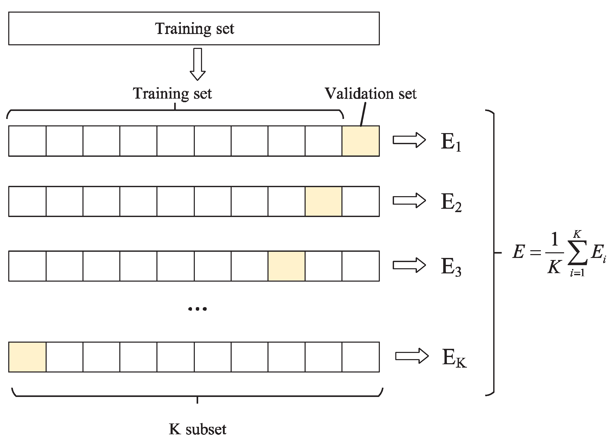
Figure 2 shows the intuitive diagram of the K-fold cross-validation. As can be seen from the figure, the original data is firstly divided into the training and validation sets. The training set is used for base model training, and the validation set is used to test the model prediction capability. The detailed step of K-fold cross-validation can be seen as follows.
Step 1:
The training set is randomly divided into K disjoint subsets;
Step 2:
The 1st and K-1th subsets are used as the training set, and the Kth subset is used as the verification set. Then, the prediction accuracy of the K group subset is calculated;
Step 3:
The second to Kth group subsets are used as the training set, and the first group subset is used as the verification set to obtain the prediction accuracy of the Kth group subset test;
Step 4:
The average prediction accuracy of the above K model is taken as the performance index of the model under K-fold cross-validation.

3. Case Study

3.1. Project Description

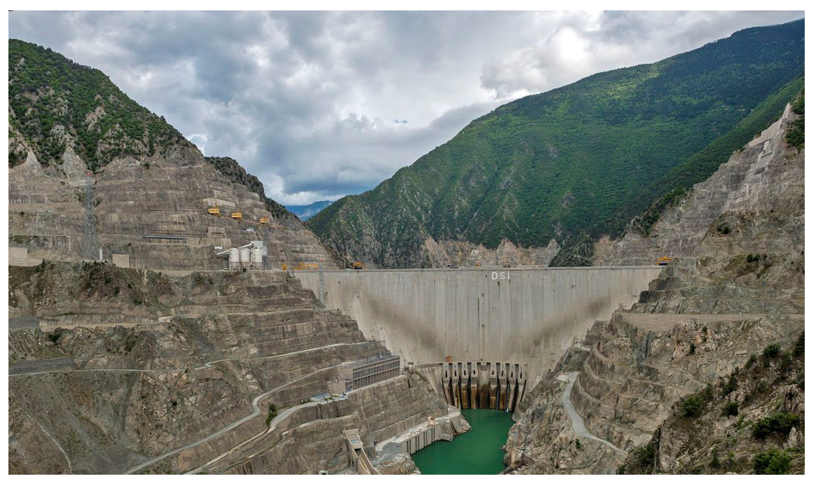
An arch dam that has been in operation for many years was used as the case study. Figure 3 shows the top view of the arch dam used in this case study. The construction of this project was started in 1968, and completed in 1971. Then, the dam was further heightened by 6.5 m in 1976 after experiencing flooding. From April 1999 to May 2000, the project was reinforced. The left and right abutments were grouted for leakage control and corresponding management facilities were implemented.
The control drainage area of the dam site is 165 km2, and the annual average rainfall is 650 mm. The design flood level of the dam is 481.75 m, and the dam foundation elevation is 389.5 m. The total storage capacity of the reservoir is 16.6 million m3. The dam is a concrete gravity arch dam with a fixed center and variable radius. The dam crest arc length is 154.28 m, and the dam crest central angle is 80°. The outer radius is 110.5 m, and the dam crest elevation is 490.5 m. The maximum dam height is 202 m, and the dam crest thickness is 4.5 m.
To monitor the environmental loads related to dam structural behavior, a series of sensors were embedded in the dam body and its foundation to monitor physical quantities, such as temperatures, water level, and rainfall. Figure 4 shows the layout of parts of thermometer monitoring points in the typical dam section. As can be seen from the image, thermometers are arranged along the dam to monitor the temperature variation in different elevations.
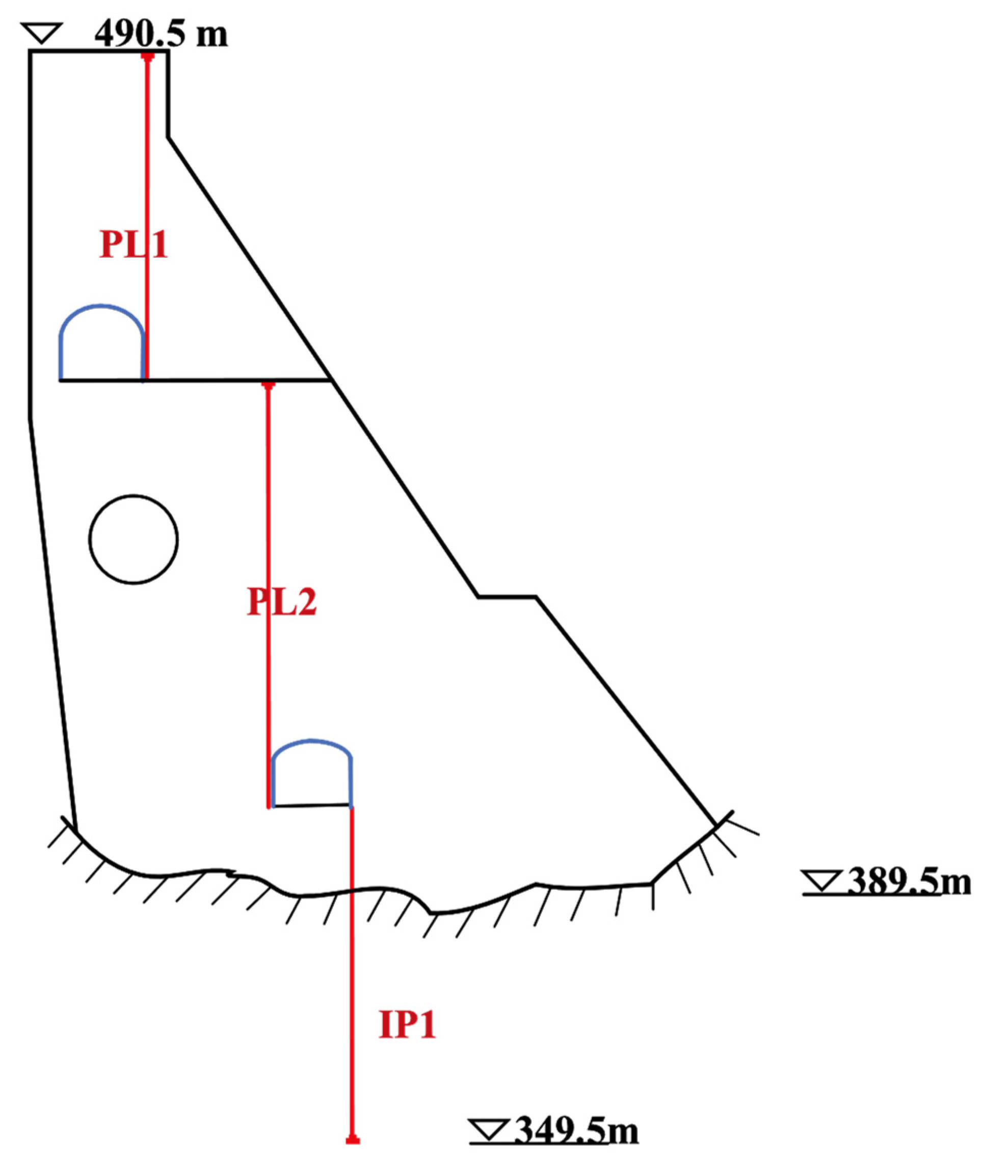
Deformation is the most intuitive monitoring indicator of structural behavior changes in arch dams. A plumb line system is utilized to monitor the horizontal displacement of the dam body and its foundation in different elevations. Figure 5 shows the typical monitoring point layout of PL and IP in this project. A total of two PL monitoring points and one IP monitoring point are utilized to measure the dam body deformation relative to the dam foundation.

3.2. Data Collection and Preprocessing

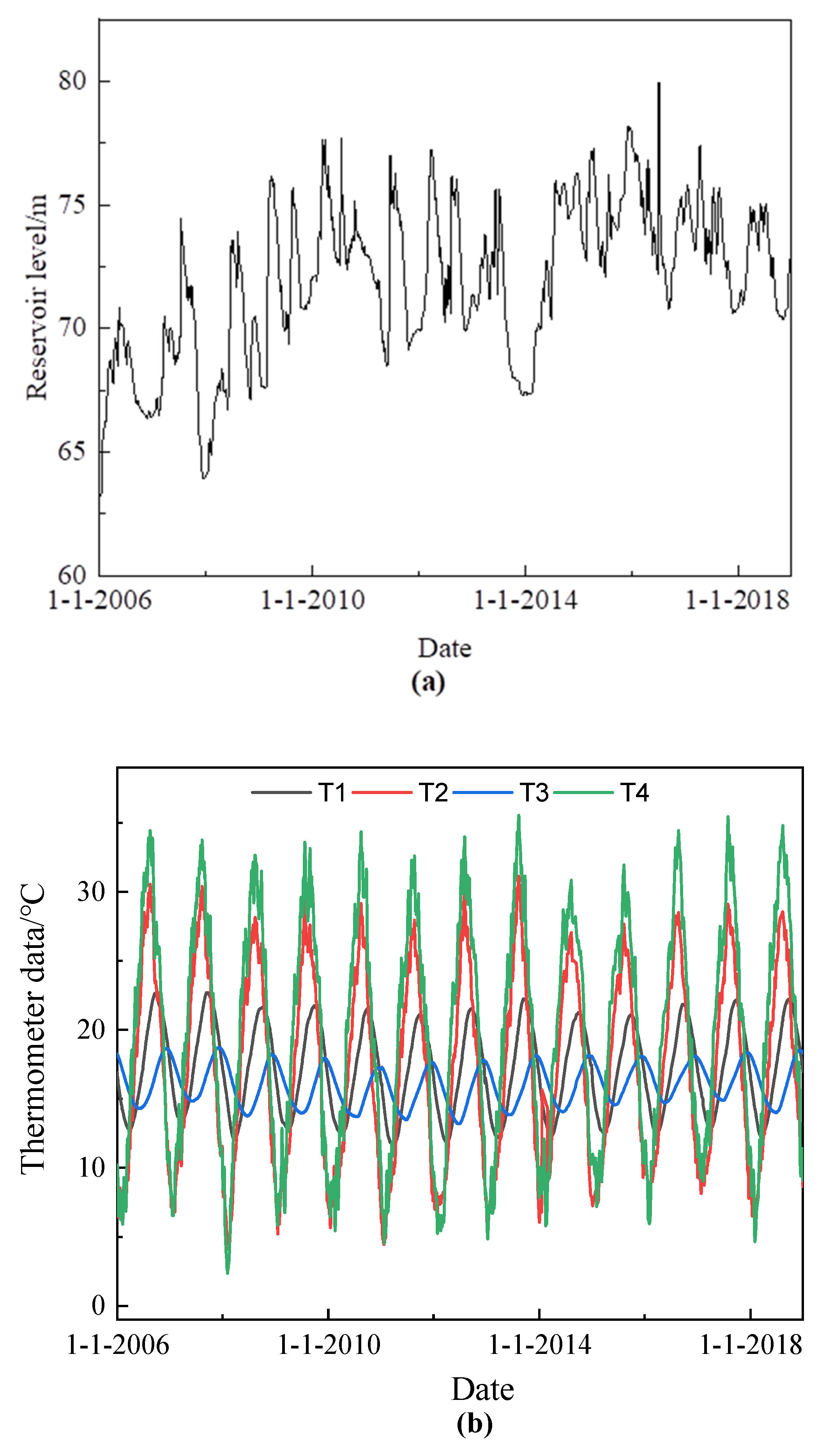
In this study, actual temperature monitoring data was used for data-driven model construction. To monitor the actual temperature field distribution and the temperature changes in different parts, a series of thermometers are embedded. In this study, the actual monitoring data from a total of 30 thermometers was utilized for model construction. Figure 6 shows the process line diagram of environmental variables (i.e., water level and temperature) from 2006 to 2018. It can be seen from the figure that both water level and temperature data show regular changes in the annual cycle. However, it can also be seen that the monitoring data of different thermometers have significant differences in amplitude, which is mainly due to the differences in their buried positions and corresponding monitoring targets. Figure 7 shows the visual display of dam displacement time series of three typical monitoring points, including PL01, PL02, and IP01. It can be seen from the figure that the fluctuation of the displacement monitoring data of the PL is significantly larger than that of the inverted vertical line, which is mainly due to the monitoring of the displacement of the dam body and the displacement of the dam foundation monitored by the IP.

3.3. Experiment Environment Setting and Parameter Tuning

The software environment of the experiment and the configuration of the corresponding parameters is shown as follows. The proposed BO–LGB and benchmark methods were coded based on Python, and all the experiments were implemented on a PC server. The server configuration is Intel 7700 k,1 GPU is Nvidia GTX1070, and memory is 16 GB.
The selection of setting parameters will significantly affect the model performance of LGB. Table 1 shows the main six parameters of LGB that mainly determine the fitting capability of LGB and the corresponding parameter optimization scale. The details about these parameters can be seen as follows. n _ e s t i m a t o r determines the depth of the tree, and a high value can enhance the model learning capability, but a too large value may also lead to model overfitting phenomenon. max _ d e p t h controls the maximum depth of the tree, which is capable of handing model overfitting. The parameter setting of f e a t u r e _ f r a c t i o n _ r a t e determines the subsampling of features. The combination implementation of both f e a t u r e _ f r a c t i o n _ r a t e and b a g g i n g _ f r a c t i o n can accelerate the model calculation process and reduce overfitting.
To further evaluate the model performance of the proposed method, a series of statistical and ML-based methods were utilized as the benchmark methods. These methods include the HST model, support vector machine (SVM), artificial neural network (ANN), random forest regression (RF), and gaussian process regression (GP). It should be noted that, except for the HST model, the input variables of the other benchmark methods were based on HTT models, i.e., hydraulic, thermal, and time-varying variables. The random search optimization algorithm was used to find the optimal parameters and training and validation data were the same as the proposed method.
In this study, three quantitative evaluation indicators, including correlation coefficients (R2), mean absolute error (MAE), and root mean squared error (RMSE) were introduced to assess the prediction performance of the proposed and the benchmark models. The formulas of these indicators can be represented as follows.
R 2 = 1 i = 1 n ( y i y ^ i ) 2 i = 1 n ( y i y ¯ ) 2
M A E = 1 n i = 1 n | y i y ^ i |
R M S E = 1 n i = 1 n | y i y ^ i | 2
where y ^ i is the predicted value of the i-th sample, y i is the corresponding actual value for total n samples, and y ¯ = 1 n i = 1 n y i .

4. Results Discussion

4.1. Project Description

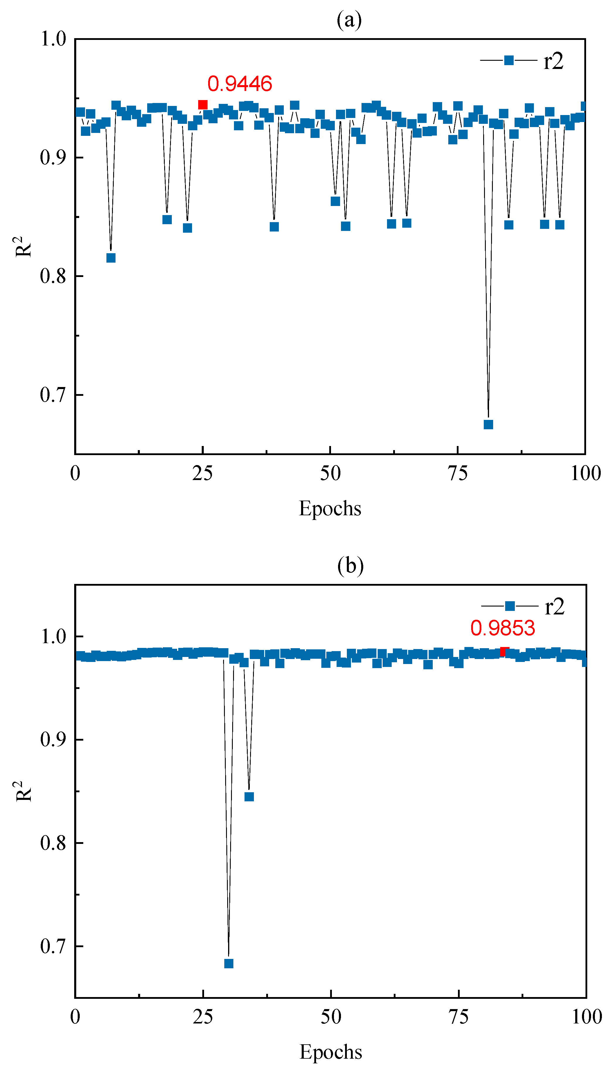
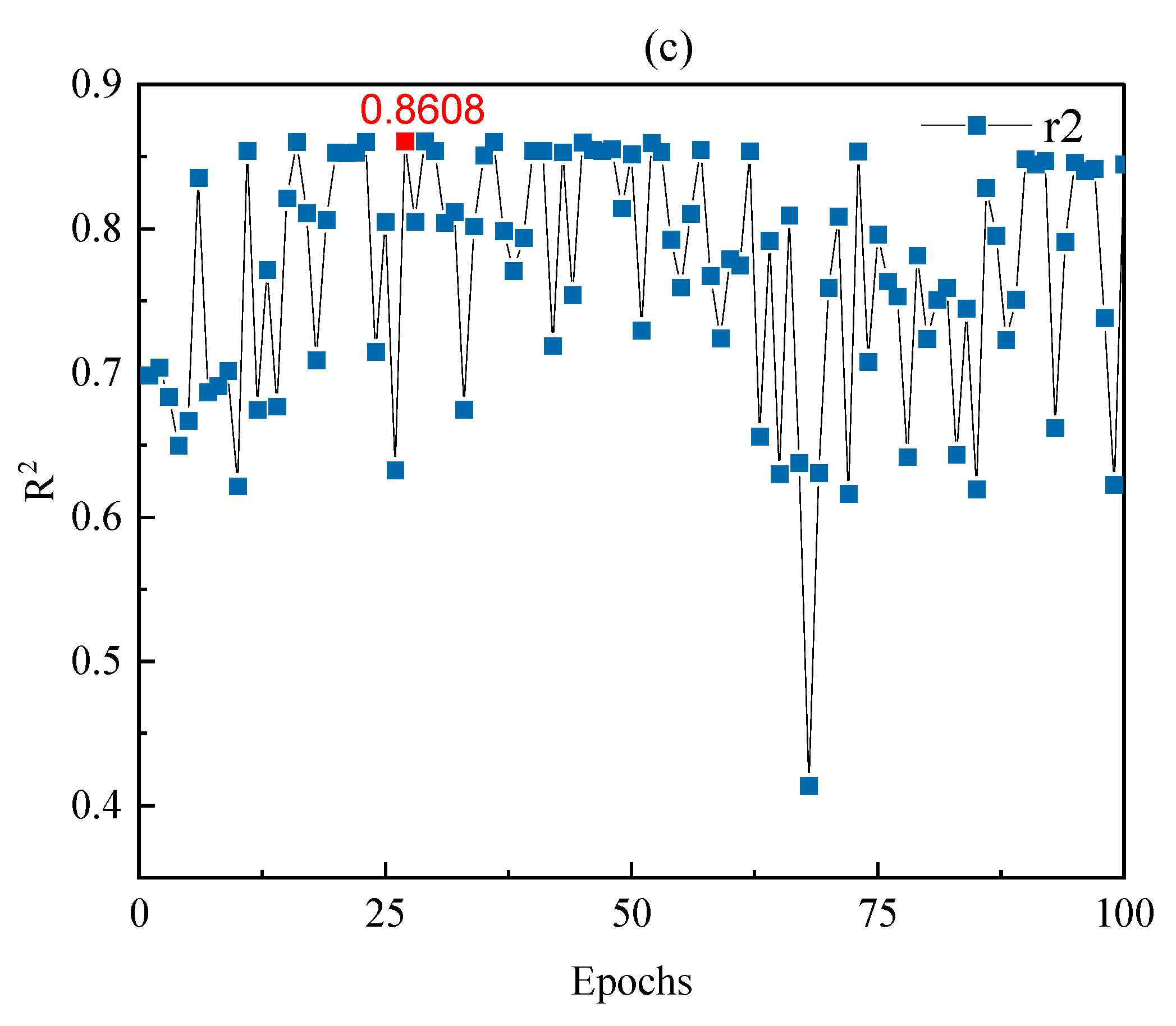
In this study, two PL monitoring points and one IP monitoring point were used to validate the model prediction capability of the proposed model. A BO parameter tuning strategy was used to determine the optimal parameters of LGB. Figure 8 shows the visual display of BO optimization results for the three monitoring points. Table 2 shows the corresponding parameter optimization results. It can be seen from the table that the optimal parameter can be obtained after 25, 84, and 27 iterations for monitoring points PL1, PL2, and IP1. The correlation coefficients in the validation sets are 0.9446, 0.9853, and 0.8608, respectively.

4.2. Model Generalization Capability Evaluation

In this study, the model performance evaluation was mainly carried out considering three parts: prediction accuracy for both short-term and long-term prediction periods, and the prediction efficiency for large-scale monitoring data.

4.2.1. Short-Term Prediction Performance Evaluation

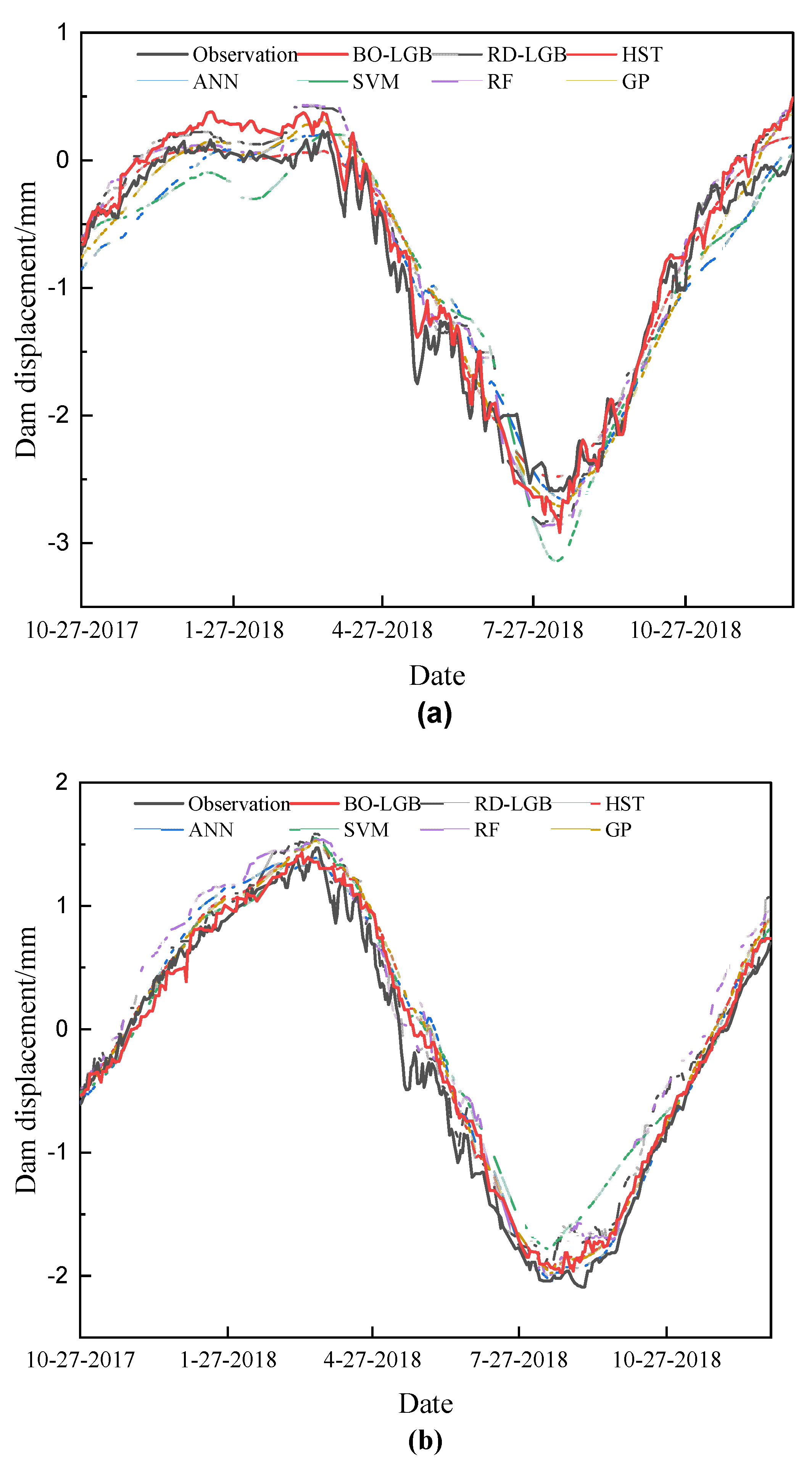
Short-term prediction of dam displacement is an important basic work for dam safety management. To verify the predictive performance of the proposed model, a series of comparative models, including RD_LGB, HST, ANN, SVM, RF, and GP, were used as the benchmark methods. Table 3 shows the quantitative evaluation comparison of the proposed and comparative methods in three monitoring points. It can be inferred from the table that the proposed method shows better short-term prediction performance in terms of all three quantitative evaluation indicators. Moreover, it can be seen that the prediction accuracy of the BO–LGB model is significantly higher than the RD–LGB model. This indicates that the BO algorithm can easily find the optimal solution under a limited number of iterations. Figure 9 shows the visual comparison of the prediction results of the proposed and comparative method. From the figure, it can be seen that the prediction values of the BO–LGB model are closer to the actual observed values.

4.2.2. Long-Term Prediction Performance Evaluation

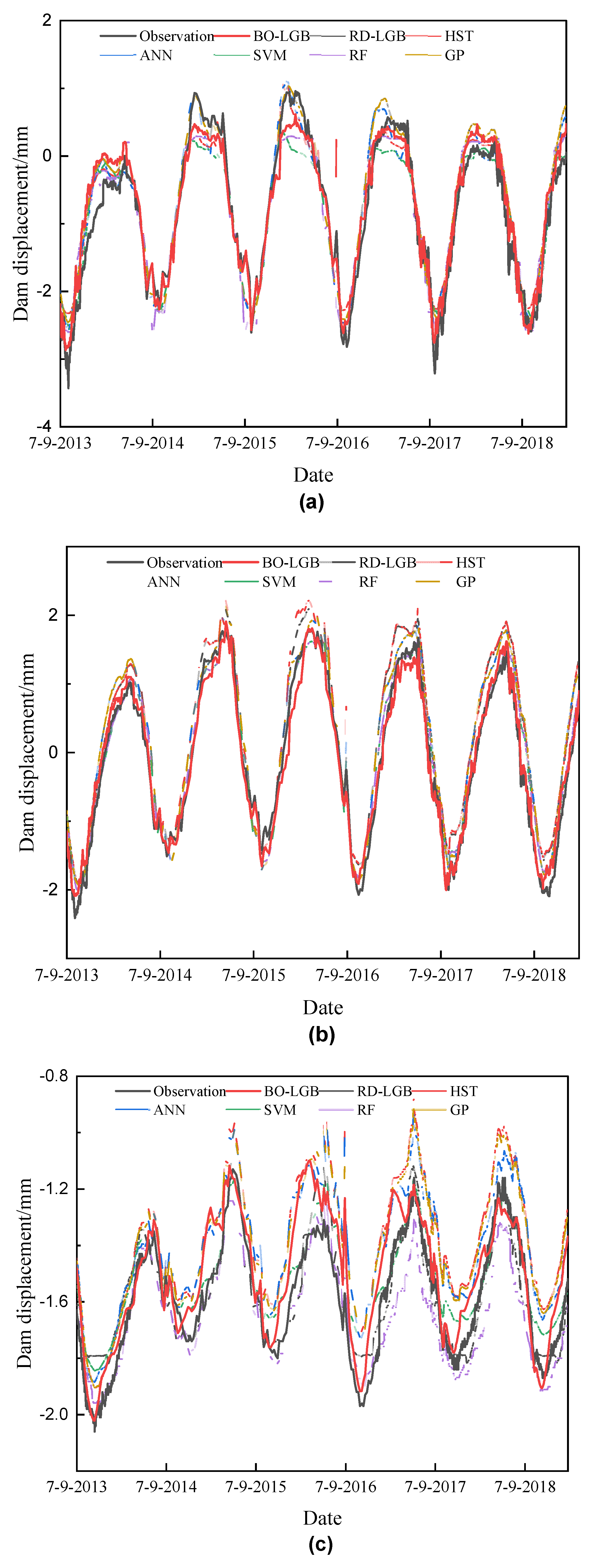
With the increase of the dam service period, the monitoring data related to the dam operation period continues to increase. Table 4 shows the quantitative result evaluation of the proposed and comparative methods in dam long-term displacement prediction. Figure 10 shows the intuitive display of the proposed and comparative methods in long-term prediction. It can be inferred that the proposed BO–LGB shows significant advantages in dam displacement sequence long-term prediction. Thust is can be concluded that, benefiting from the comprehensive application of the BO algorithm and the five-fold cross-validation technology, the proposed model can fully mine the underlying information related to dam displacement changes in the limited monitoring data.

4.3. Model Interpretability Assessment

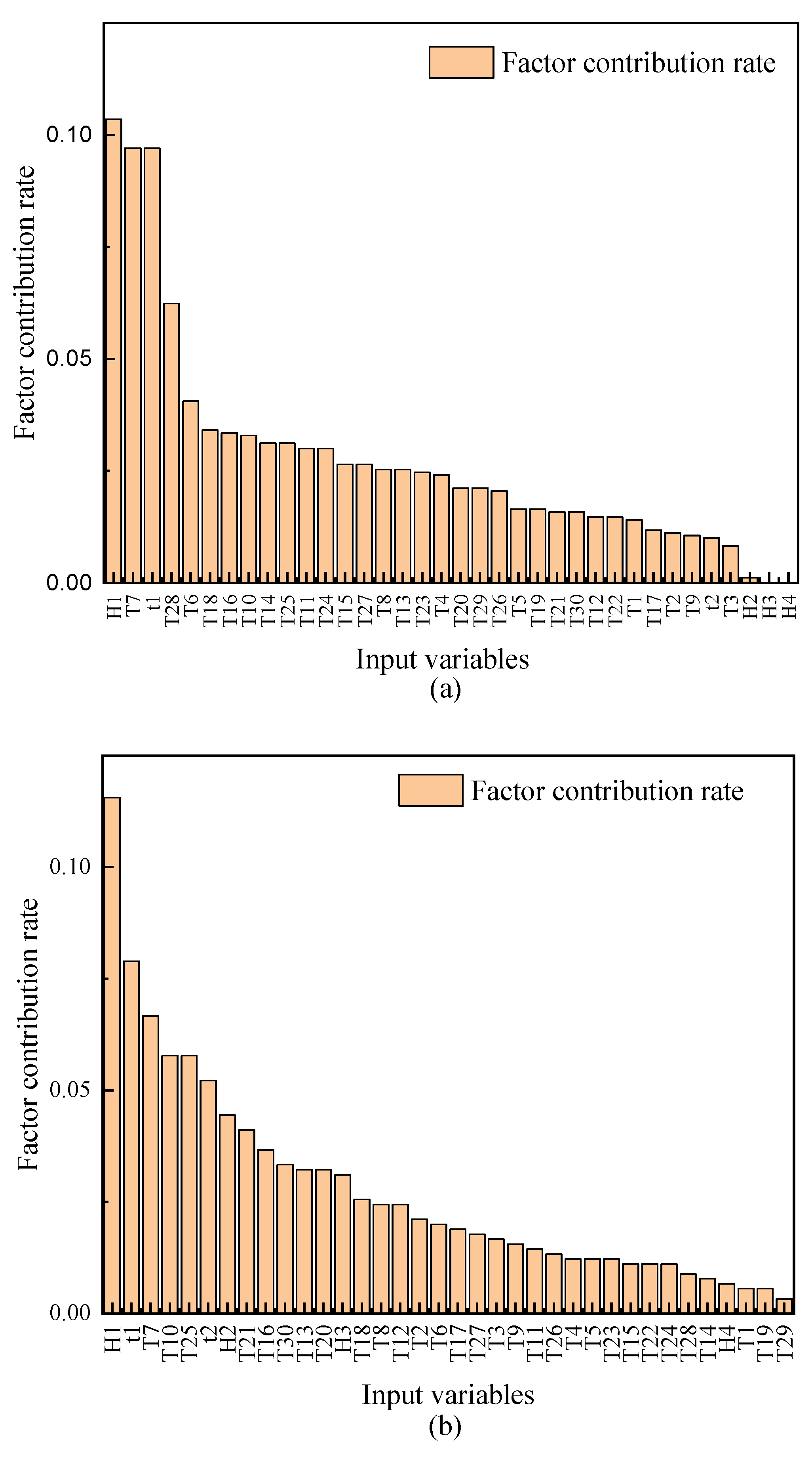
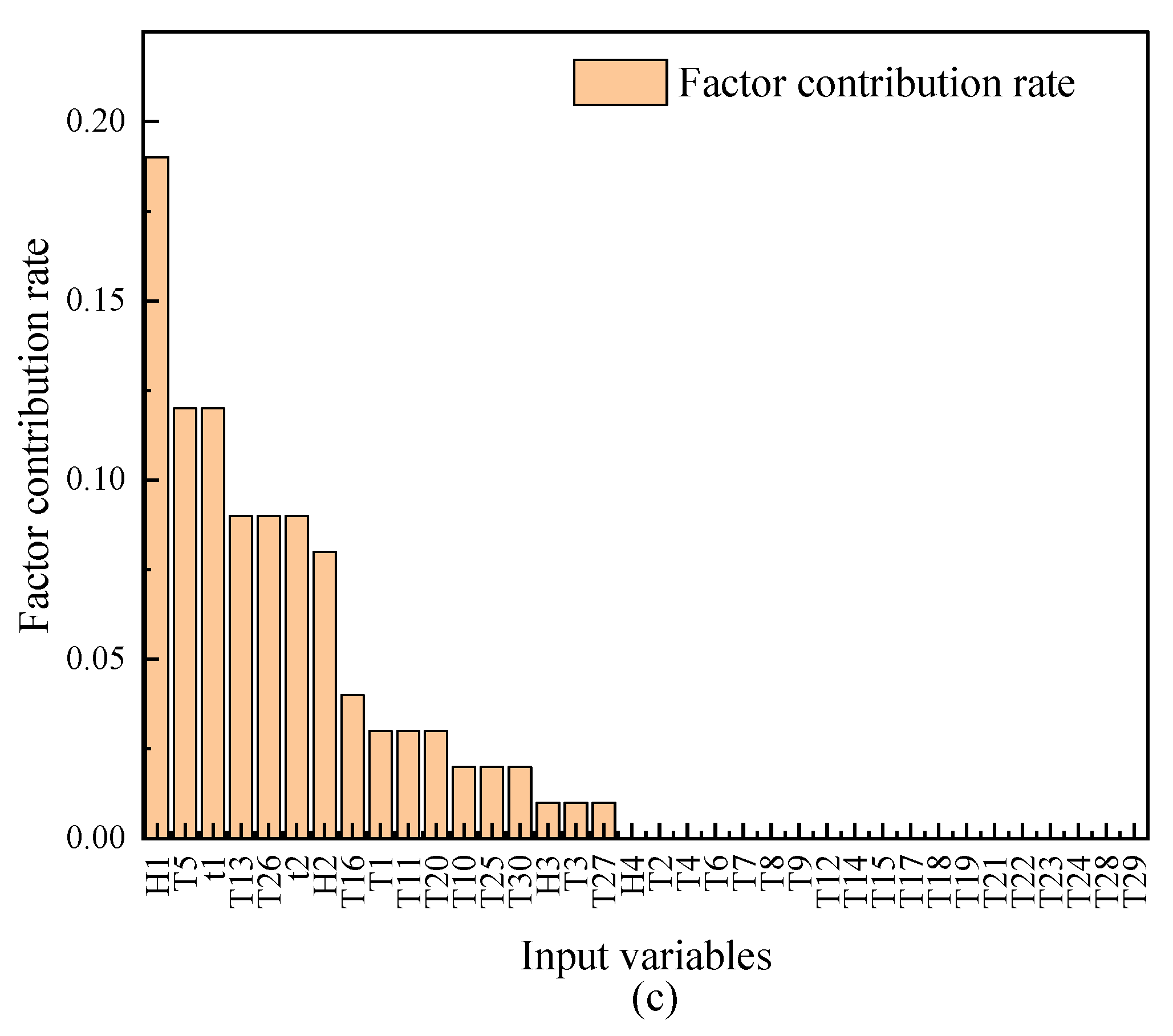
A significant feature of the HTT model is the high dimension of the factor. Figure 11 shows the visual display of factor importance in input variables for the three monitoring points. It can be seen from the figure that the water level factor is the most important factor affecting the dam displacement changes for all three monitoring points. Moreover, temperature data has a significant impact on the dam displacement changes. However, the monitoring points embedded in different positions are affected by the temperature variation. Thus, it is desirable to select the thermometers with a high relationship with dam deformation according to the interpretation results of BO–LGB.

5. Conclusions

In this study, a dam displacement prediction, monitoring, and interception model was proposed based on LGB and BO algorithms. Different from the conventional HST model, the proposed method directly takes the prototypical dam environmental monitoring data as the input variables. LGB is combined with the BO algorithm to build a dam deformation monitoring and interpretation model using long-term prototypical monitoring data. The main contributions of this paper are summarized as follows.
  • The proposed BO–LGB model shows strong capability when dealing with the long-term dam monitoring data both in modeling accuracy and efficiency;
  • The proposed method achieves remarkable performance in a variety of dam displacement prediction scenarios (both in short-term prediction and long-term prediction);
  • The proposed method can analyze the main factors affecting dam displacement changes based on prototypical monitoring data.
However, some limitations should also be addressed. First of all, the research object of this study was a concrete dam, but other dam types like earth-rock dams or face rockfill dams should also be used as research items. Secondly, since dam displacement is an uncertain process affected by many factors, the stimulation of the uncertainty is an important research content. There is a certain degree of correlation between different dam monitoring points. The main research in the future is to consider the correlation between multiple monitoring points and other types of dams.

Author Contributions

Conceptualization, methodology, software, funding, P.H.; validation, formal analysis, investigation, resources, Y.L. All authors have read and agreed to the published version of the manuscript.

Funding

This research has been supported by the Open Fund of the Key Laboratory of River Channel and Estuary Management in the Lower Yellow River of the Ministry of Water Resources: LYRCER202103.

Conflicts of Interest

The authors declare no conflict of interest.

References

  1. Kang, F.; Li, J.; Zhao, S.; Wang, Y. Structural health monitoring of concrete dams using long-term air temperature for thermal effect simulation. Eng. Struct. 2019, 180, 642–653. [Google Scholar] [CrossRef]
  2. Kang, F.; Li, J. Displacement Model for Concrete Dam Safety Monitoring via Gaussian Process Regression Considering Extreme Air Temperature. J. Struct. Eng. 2020, 146, 05019001. [Google Scholar] [CrossRef]
  3. Tatin, M.; Briffaut, M.; Dufour, F.; Simon, A.; Fabre, J.-P. Thermal displacements of concrete dams: Accounting for water temperature in statistical models. Eng. Struct. 2015, 91, 26–39. [Google Scholar] [CrossRef]
  4. Kang, F.; Liu, X.; Li, J. Concrete Dam Behavior Prediction Using Multivariate Adaptive Regression Splines with Meas-ured Air Temperature. Arab. J. Sci. Eng. 2019, 44, 8661–8673. [Google Scholar] [CrossRef]
  5. Li, Y.; Bao, T.; Shu, X.; Chen, Z.; Gao, Z.; Zhang, K. A Hybrid Model Integrating Principal Component Analysis, Fuzzy C-Means, and Gaussian Process Regression for Dam Deformation Prediction. Arab. J. Sci. Eng. 2020, 46, 4293–4306. [Google Scholar] [CrossRef]
  6. Liu, J.; Zhou, X.C.; Chen, W.; Hong, X. Breach Discharge Estimates and Surface Velocity Measurements for an Earth Dam Failure Process Due to Overtopping Based on the LS-PIV Method. Arab. J. Sci. Eng. 2019, 44, 329–339. [Google Scholar] [CrossRef]
  7. Ma, C.; Gao, Z.; Yang, J.; Cheng, L.; Chen, L. Operation Performance and Seepage Flow of Impervious Body in Blast-Fill Dams Using Discrete Element Method and Measured Data. Water 2022, 14, 1443. [Google Scholar] [CrossRef]
  8. Tong, F.; Yang, J.; Ma, C.; Cheng, L.; Li, G. The Prediction of Concrete Dam Displacement Using Copula-PSO-ANFIS Hybrid Model. Arab. J. Sci. Eng. 2022, 47, 4335–4350. [Google Scholar] [CrossRef]
  9. Salazar, F.; Toledo, M.; Oñate, E.; Morán, R. An empirical comparison of machine learning techniques for dam behaviour modelling. Struct. Saf. 2015, 56, 9–17. [Google Scholar] [CrossRef]
  10. Xi, R.; Zhou, X.; Jiang, W.; Chen, Q. Simultaneous estimation of dam displacements and reservoir level variation from GPS measurements. Measurement 2018, 122, 247–256. [Google Scholar] [CrossRef]
  11. Liu, H.Z.; Wang, S.L.; Liu, J.Y. LS-SVM Prediction Model Based on Phase Space Reconstruction for Dam Deformation. Adv. Mater. Res. 2013, 663, 55–59. [Google Scholar] [CrossRef]
  12. Shao, C.; Gu, C.; Yang, M.; Xu, Y.; Su, H. A novel model of dam displacement based on panel data. Struct. Control Health Monit. 2018, 25, e2037. [Google Scholar] [CrossRef]
  13. Yang, L.; Su, H.; Wen, Z. Improved PLS and PSO methods-based back analysis for elastic modulus of dam. Adv. Eng. Softw. 2019, 131, 205–216. [Google Scholar] [CrossRef]
  14. Li, B.; Yang, J.; Hu, D. Dam monitoring data analysis methods: A literature review. Struct. Control Health Monit. 2020, 27, e2501. [Google Scholar] [CrossRef]
  15. Thangam, Y.Y.; Kalanithi, M.; Anbarasi, C.M.; Rajendran, S. Inhibition of Corrosion of Carbon Steel in a Dam Water by Sodium Molybdate–Zn2+ System. Arab. J. Sci. Eng. 2009, 34, 49–60. [Google Scholar]
  16. Lin, C.; Li, T.; Chen, S.; Liu, X.; Lin, C.; Liang, S. Gaussian process regression-based forecasting model of dam deformation. Neural Comput. Appl. 2019, 31, 8503–8518. [Google Scholar] [CrossRef]
  17. Qu, X.; Yang, J.; Chang, M. A Deep Learning Model for Concrete Dam Deformation Prediction Based on RS-LSTM. J. Sens. 2019, 2019, 4581672. [Google Scholar] [CrossRef]
  18. Mata, J.; de Castro, A.T.; da Costa, J.S. Constructing Statistical Models for Arch Dam Deformation. Struct. Control Health Monit. 2014, 21, 423–437. [Google Scholar] [CrossRef]
  19. Su, H.; Li, X.; Yang, B.; Wen, Z. Wavelet support vector machine-based prediction model of dam deformation. Mech. Syst. Signal Process. 2018, 110, 412–427. [Google Scholar] [CrossRef]
  20. Beaujoint, N.J. Discussion of “Dead Load Stress in Model Dams by Method of Integration”. J. Struct. Div. 1962, 88, 317–318. [Google Scholar] [CrossRef]
  21. Belmokre, A.; Mihoubi, M.K.; Santillán, D. Analysis of Dam Behavior by Statistical Models: Application of the Random Forest Approach. KSCE J. Civ. Eng. 2019, 23, 4800–4811. [Google Scholar] [CrossRef]
  22. Salazar, F.; Morán, R.; Toledo, M.; Oñate, E. Data-Based Models for the Prediction of Dam Behaviour: A Review and Some Methodological Considerations. Arch. Comput. Methods Eng. 2017, 24, 1–21. [Google Scholar] [CrossRef]
  23. Hu, J.; Wu, S. Statistical modeling for deformation analysis of concrete arch dams with influential horizontal cracks. Struct. Health Monit. 2019, 18, 546–562. [Google Scholar] [CrossRef]
  24. Wieland, M.; Kirchen, G.F. Long-term dam safety monitoring of Punt dal Gall arch dam in Switzerland. Front. Struct. Civ. Eng. 2012, 6, 76–83. [Google Scholar] [CrossRef]
  25. Li, M.; Shen, Y.; Ren, Q.; Li, H. A new distributed time series evolution prediction model for dam deformation based on constituent elements. Adv. Eng. Inform. 2019, 39, 41–52. [Google Scholar] [CrossRef]
  26. Ren, Q.; Li, M.; Song, L.; Liu, H. An optimized combination prediction model for concrete dam deformation considering quantitative evaluation and hysteresis correction. Adv. Eng. Inform. 2020, 46, 101154. [Google Scholar] [CrossRef]
  27. Li, Y.; Bao, T.; Gong, J.; Shu, X.; Zhang, K. The Prediction of Dam Displacement Time Series Using STL, Extra-Trees, and Stacked LSTM Neural Network. IEEE Access 2020, 8, 94440–94452. [Google Scholar] [CrossRef]
  28. Bui, K.-T.T.; Tien Bui, D.; Zou, J.; Van Doan, C.; Revhaug, I. A novel hybrid artificial intelligent approach based on neural fuzzy inference model and particle swarm optimization for horizontal displacement modeling of hydropower dam. Neural Comput. Appl. 2018, 29, 1495–1506. [Google Scholar] [CrossRef]
  29. Li, X.; Wen, Z.; Su, H. An approach using random forest intelligent algorithm to construct a monitoring model for dam safety. Eng. Comput. 2021, 37, 39–56. [Google Scholar] [CrossRef]
  30. Milillo, P.; Perissin, D.; Salzer, J.T.; Lundgren, P.; Lacava, G.; Milillo, G.; Serio, C. Monitoring dam structural health from space: Insights from novel InSAR techniques and multi-parametric modeling applied to the Pertusillo dam Basilicata, Italy. Int. J. Appl. Earth Obs. Geoinf. 2016, 52, 221–229. [Google Scholar] [CrossRef]
  31. Ribeiro, L.S.; Wilhelm, V.E.; Faria, F.; Correa, J.M.; dos Santos, A.C.P. A comparative analysis of long-term concrete deformation models of a buttress dam. Eng. Struct. 2019, 193, 301–307. [Google Scholar] [CrossRef]
  32. Gui, G.; Pan, H.; Lin, Z.; Li, Y.; Yuan, Z. Data-driven support vector machine with optimization techniques for structural health monitoring and damage detection. KSCE J. Civ. Eng. 2017, 21, 523–534. [Google Scholar] [CrossRef]
  33. Ma, J.; Cheng, J.C.; Jiang, F.; Chen, W.; Wang, M.; Zhai, C. A bi-directional missing data imputation scheme based on LSTM and transfer learning for building energy data. Energy Build. 2020, 216, 109941. [Google Scholar] [CrossRef]
  34. Malekloo, A.; Ozer, E.; AlHamaydeh, M.; Girolami, M. Machine Learning and Structural Health Monitoring Overview with Emerging Technology and High-Dimensional Data Source Highlights. Struct. Health Monit. 2022, 21, 1906–1955. [Google Scholar] [CrossRef]
  35. Chen, S.; Gu, C.; Lin, C.; Zhao, E.; Song, J. Safety Monitoring Model of a Super-High Concrete Dam by Using RBF Neural Network Coupled with Kernel Principal Component Analysis. Math. Probl. Eng. 2018, 2018, 1712653. [Google Scholar] [CrossRef]
  36. Su, Y.; Weng, K.; Lin, C.; Zheng, Z. An Improved Random Forest Model for the Prediction of Dam Displacement. IEEE Access 2021, 9, 9142–9153. [Google Scholar] [CrossRef]
  37. Ren, Q.; Li, M.; Li, H.; Song, L.; Si, W.; Liu, H. A robust prediction model for displacement of concrete dams subjected to irregular water-level fluctuations. Comput. -Aided Civ. Infrastruct. Eng. 2021, 36, 577–601. [Google Scholar] [CrossRef]
  38. Li, M.; Li, M.; Ren, Q.; Li, H.; Song, L. DRLSTM: A dual-stage deep learning approach driven by raw monitoring data for dam dis-placement prediction. Adv. Eng. Inform. 2022, 51, 101510. [Google Scholar] [CrossRef]
  39. Ren, Q.; Li, M.; Kong, T.; Ma, J. Multi-sensor real-time monitoring of dam behavior using self-adaptive online sequential learning. Autom. Constr. 2022, 140, 104365. [Google Scholar] [CrossRef]
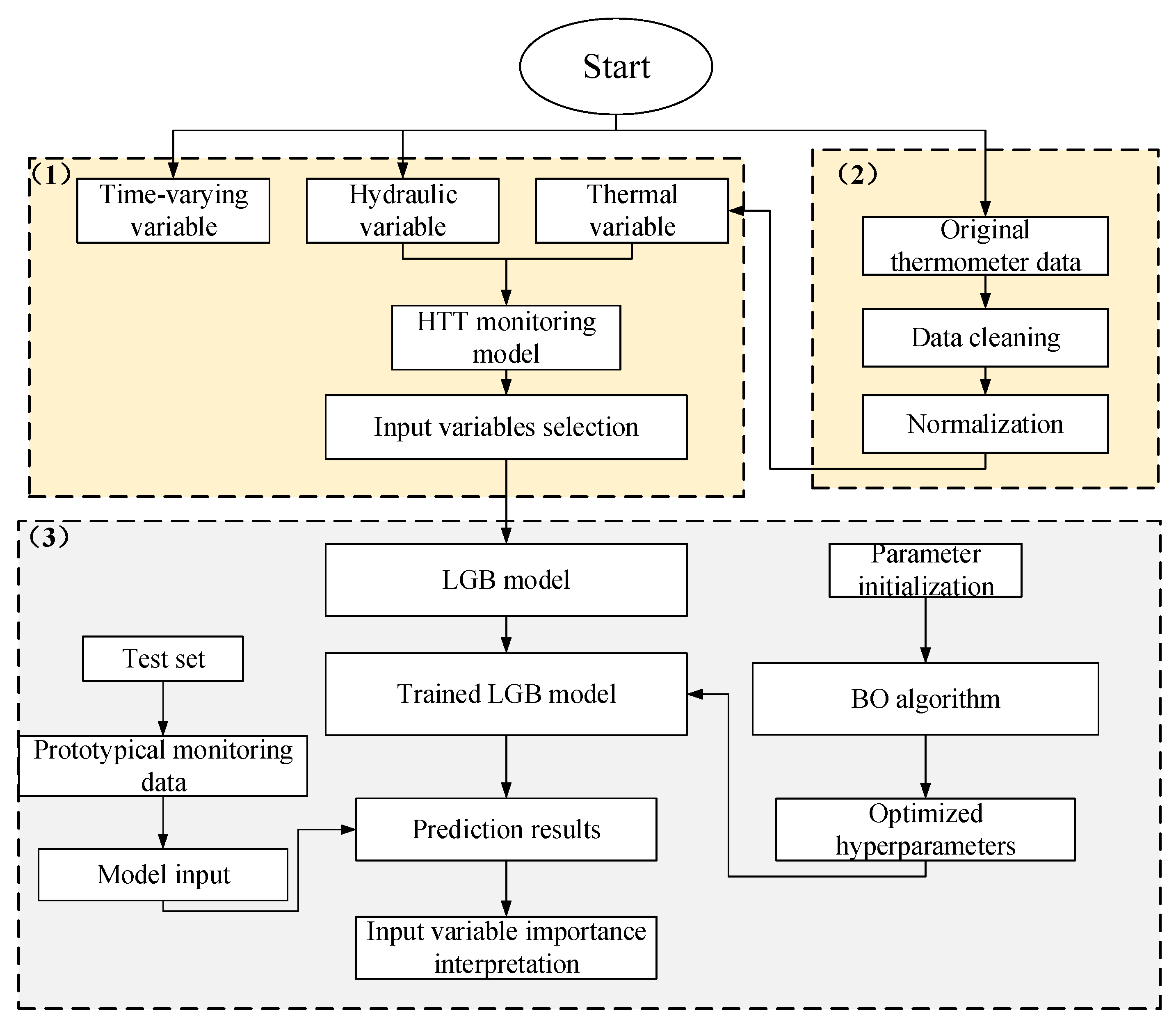
Figure 1. The flowchart of the proposed framework.
Water 14 02538 g001
Figure 2. K-fold cross-validation diagram.
Water 14 02538 g002
Figure 3. Top view of the arch dam used in this case study.
Water 14 02538 g003
Figure 4. Thermometer layout of typical dam sections.
Water 14 02538 g004
Figure 5. The arrangement of the PL and IP monitoring system.
Water 14 02538 g005
Figure 6. Intuitive display of environmental variable process: (a) reservoir level process, (b) thermometer data.
Water 14 02538 g006
Figure 7. Visual display of three dam absolute displacement monitoring data from 2006 to 2018.
Water 14 02538 g007
Figure 8. Visual display of BO parameter tuning results: (a) PL01, (b) PL02, and (c) IP01.
Water 14 02538 g008aWater 14 02538 g008b
Figure 9. Intuitive comparison of the prediction results of the proposed and the benchmark methods at the typical three monitoring points. (a) PL01, (b) PL02, and (c) IP01.
Water 14 02538 g009aWater 14 02538 g009b
Figure 10. Intuitive comparison of the prediction results of the proposed and benchmark methods at the typical three monitoring points. (a) PL01, (b) PL02, and (c) IP01.
Water 14 02538 g010
Figure 11. Factor importance assessment results of three typical monitoring sites: (ac) denotes monitoring points PL1, PL2, and IP01.
Water 14 02538 g011aWater 14 02538 g011b
Table 1. The parameter optimization objects in LGB.
ParametersParameter Optimization Range
n _ e s t i m a t o r [ 10 , 500 ]
n u m _ l e a v e s [ 10 , 100 ]
min _ c h i l d _ s a m p l e s [ 1 , 20 ]
max _ d e p t h [ 1 , 100 ]
f e a t u r e _ f r a c t i o n _ r a t e [ 0.5 , 0.9999 ]
b a g g i n g _ f r a c t i o n [ 0.5 , 0.9999 ]
Table 2. The parameter optimization results of BO for LGB.
n_Estimatorsnum_Leavesmin_Child_SamplesMax_DepthFeature_FractionBagging_Fraction
PL01474199500.960.67
PL025001020730.50.5
IP01424481720.730.89
Table 3. The comparison of short-term dam displacement prediction performance of the proposed and benchmark methods.
ProposedRD_LGBHSTANNSVMRFGP
PL01R20.9600 0.9238 0.9490 0.9103 0.8739 0.9243 0.9323
MSE0.1920 0.2689 0.1950 0.2532 0.3171 0.2666 0.2440
MAE0.1622 0.2226 0.1378 0.2057 0.2598 0.2106 0.1882
PL02R20.9703 0.9638 0.9621 0.9607 0.3334 0.9289 0.9608
MSE0.1751 0.1928 0.2072 0.1981 0.7291 0.2806 0.2104
MAE0.1327 0.1641 0.1591 0.1423 0.6231 0.2474 0.1589
IP01R20.9855 0.9836 0.8879 0.8796 0.5692 0.8499 0.9354
MSE0.0269 0.0284 0.0688 0.0678 0.1198 0.0764 0.0528
MAE0.0217 0.0227 0.0633 0.0573 0.1120 0.0663 0.0480
Table 4. Performance comparison of the proposed and comparative methods in long-term dam displacement prediction.
ProposedRD_LGBHSTANNSVMRFGP
PL01R20.90670.8703 0.8669 0.8833 0.8656 0.8746 0.8703
MSE0.3044 0.3708 0.3354 0.3354 0.3306 0.3440 0.3708
MAE0.2472 0.3158 0.2801 0.2758 0.2578 0.2793 0.3158
PL02R20.9724 0.8505 0.8390 0.8737 0.9454 0.9454 0.8737
MSE0.1804 0.4542 0.4753 0.4179 0.2559 0.2559 0.4179
MAE0.1490 0.4151 0.4348 0.3723 0.1942 0.1942 0.3723
IP01R20.7792 0.7734 0.2823 0.3622 0.6911 0.6186 0.3518
MSE0.1064 0.0932 0.2139 0.1853 0.0968 0.1114 0.1976
MAE0.0825 0.0770 0.2028 0.1736 0.0793 0.0925 0.1884
Publisher’s Note: MDPI stays neutral with regard to jurisdictional claims in published maps and institutional affiliations.