Article

Network Subsystems for Robust Design Optimization of Water Distribution Systems

Faculty of Civil and Environmental Engineering, Technion-Israel Institute of Technology, Haifa 320000, Israel
*
Author to whom correspondence should be addressed.
Water 2022, 14(15), 2443; https://doi.org/10.3390/w14152443
Submission received: 4 July 2022 / Revised: 3 August 2022 / Accepted: 4 August 2022 / Published: 7 August 2022
(This article belongs to the Section Urban Water Management)

Abstract

:
The optimal design of WDS has been extensively researched for centuries, but most of these studies have employed deterministic optimization models, which are premised on the assumption that the parameters of the design are perfectly known. Given the inherently uncertain nature of many of the WDS design parameters, the results derived from such models may be infeasible or suboptimal when they are implemented in reality due to parameter values that differ from those assumed in the model. Consequently, it is necessary to introduce some uncertainty in the design parameters and find more robust solutions. Robust counterpart optimization is one of the methods used to deal with optimization under uncertainty. In this method, a deterministic data set is derived from an uncertain problem, and a solution is computed such that it remains viable for any data realization within the uncertainty bound. This study adopts the newly emerging robust optimization technique to account for the uncertainty associated with nodal demand in designing water distribution systems using the subsystem-based two-stage approach. Two uncertainty data models with ellipsoidal uncertainty set in consumer demand are examined. The first case, referred to as the uncorrelated problem, considers the assumption that demand uncertainty only affects the mass balance constraint, while the second case, referred to as the correlated case, assumes uncertainty in demand and also propagates to the energy balance constraint.

1. Introduction

A WDS network should provide the desired service throughout its lifetime. However, the system’s overall performance is influenced by factors such as component failure (pipes, pumps, storage), aging, and fluctuations in demand. Pipe failures represent the most significant [1]. Even though pipe failures may be temporary, it is highly undesirable to experience interruptions in the supply of an essential commodity such as water. As a result, a WDS must have sufficient redundancy to meet the needs of consumers during abnormal conditions. Redundancy in a WDS network can be defined as the number of simultaneous failures that can be tolerated without resulting in a significant disruption to service [1]. There is, however, a direct correlation between the level of redundancy and the cost of the network. In spite of this, since the probability of multiple pipeline failures is low, a level-1 redundant system provides adequate protection. Level-1 redundancy refers to the ability of a network to continue providing acceptable service in the event of a component failure. Several authors have used redundancy as a measure of reliability [1,2,3,4,5,6,7,8]. Ormsbee and Kessler [1] developed a subsystem-based two-stage approach to design a level-1 redundant network in which topology and hydraulic requirements are satisfied at different stages. From a topology point of view, a level-1 redundant network requires the existence of two distinct sources to demand node paths. This requirement can be satisfied using network construction. The network is then decomposed into two subsystem groups, each representing the two distinct paths that connect the source with the nodes. The outcome of this reliability inclusion method is influenced by the pair of subsystems selected. The first phase of this study discusses subsystem selection problem.
Another equally important aspect of WDS, besides reliability, is the uncertain nature of parameters involved in the optimization of WDS design. Deterministic optimization involves making decisions based on the knowledge of all design parameter values with 100% certainty. Yet, it is inconceivable that the future could be perfectly predicted, but one should instead consider it as random or uncertain. In fact, the vast majority of real-life problems are uncertain in nature. Various types of uncertainty may be present, such as uncertainty within measurements, uncertainty in the estimation of parameters, and uncertainty regarding which processes should be included in the model. It can profoundly affect the accuracy of mathematical models when mathematical determinism and natural uncertainty are in conflict. It is frequently the case that the solution to an optimization problem is highly sensitive to the data perturbations. Therefore, disregarding the data uncertainty might result in suboptimal or even infeasible solutions. Consequently, it is important to develop a methodology that allows us to consider uncertainty when predicting the behavior of a system of great practical significance. Optimization under uncertainty refers to the branch of optimization where there is uncertainty in at least one parameter of the model. The nature of optimization under uncertainty is that decisions must be made without knowing their full consequences.
Traditionally, optimization problems that involve uncertainty have been tackled with stochastic models [9,10,11]. In the stochastic approach, which has been applied to a wide variety of problems, a probability distribution is explicitly or implicitly assigned to the unknown parameters. The choice of a particular distribution is not necessarily backed by a solid statistical basis. There may be no available statistical data concerning the phenomenon to be modeled by random variables in some instances. Different techniques of stochastic optimization have been developed; one of the goals is usually to optimize the expected value of the objective function. Solutions obtained from this model are expected to be feasible with a predefined probability of success. However, even if the assumed probability distributions coincide with real distribution, feasibility is not always guaranteed. In addition, stochastic problems are highly nonlinear, which makes them difficult computationally.
The robust optimization method is a relatively new approach for modeling uncertainty in optimization problems, which is another method used to deal with uncertainties in optimization [12]. As opposed to stochastic programming, which assumes that there is a probability-based description of uncertainty, robust optimization uses a deterministic, set-based description of uncertainty [13,14]. A robust optimization approach generates a solution that is feasible for any realization within the uncertainty bound under consideration. Most robust optimization models consider the worst possible outcome and optimize decisions accordingly. In this process, the objective is to find fixed solutions that are feasible, independent of the data and uncertain parameters. Finding the worst possible outcome constitutes a corresponding optimization problem that must be solved. In some literature, the problem of finding the worst scenario is called a subproblem.
As a result of the inherent variability associated with instantaneous water consumption, consumer demand remains a significant source of uncertainty in water distribution network design. There is a correlation between uncertainty in demand and head-flow in WDS, which, in turn, can affect the reliability of the network. This aspect should be considered when designing new water systems or upgrading existing ones. This study adopts a robust counterpart optimization approach with uncertainty in nodal demands to be tested for the optimal subsystem pairs obtained from the backup selection problem.

2. Material and Methods

This study is structured in two phases. The first phase explores graph theory and focuses on the enumeration of subsystems based on the network layout. The optimal subsystem pair is selected in the first phase. The hydraulic elements of the optimal subsystems are optimized simultaneously in the second phase, where uncertainty is incorporated into consumer demand. The uncertain problem is addressed using a robust counterpart.

2.1. Subsystem Enumeration

The network must satisfy topological requirements for level-1 redundancy prior to the backup enumeration phase. Level-1 topological redundant networks exist when each node has at least two independent pathways connecting it to the source. In the event the network does not meet this requirement, additional networks can be added. Once the network has achieved topology redundancy, a special node numbering called st-numbering is generated [15], and the subsystems are enumerated in decrement and increment order according to node numbering. In this case, the subsystems are simply tree networks, one of the groups rooted at the lowest st-numbered node and the other at the highest st-numbered network [16] developed an algorithm for enumerating all the spanning trees in a directed graph. This algorithm was employed to generate all spanning trees of both subsystem groups.

Subsystem Pair Optimization

Once the backups are generated, the last stage is subsystem pair selection and hydraulic component size optimization, where the two backups are optimized simultaneously. The optimization problem is formulated as a cost minimization requiring each backup to maintain some level of service to the consumer. The mass balance constraints are omitted since the flows for a tree network are readily known. Therefore, linear programming is sufficient to find an optimal set of diameters for a given pair of backups. The general formulation of the problem is given below.
Minimize j = 1 n p i = 1 m C ( d i ) l ij ( d i ) s . t     h i T 1 h i M i n   for   i = 1 , 2 ,   ,   nn   h i T 2 h i M i n   for   i = 1 , 2 ,   ,   nn   j = 1 n d l ij = L i for   i = 1 ,   2 ,   ,   np d i D  
where C ( d i ) is the unit cost of diameter d i ,   D is the set of available diameters, h i T 1 and h i T 2 are the head in node i   in trees one and two, respectively, h i Min is the required minimum head at node i ,   L i and l ij are the length of link i   and the length of available diameter j   in link i , respectively, nn and np are the numbers of nodes and pipelines, respectively, and m is the number of available diameters ( size   D ) .
Suppose the number of possible backup pairs is small, as is the case for a small network that is relatively expected to have a small number of possible subsystem pairs. In that case, a complete search can be conducted, so optimal backup pairs and the cost vs. minimum required head tradeoff curve can be determined easily. If, however, the number of backup pairs is significantly large in order for a complete search to be conducted, as is the case for a large network that is relatively expected to have a large number of possible subsystem pairs, a heuristic search must be performed for the backup pair selection problem. The NSGAII was employed to tackle this challenge.

2.2. Robust Counterpart Optimization

Robust counterpart is an important technique for solving optimization problems involving uncertain data. In this technique, a deterministic set of data is defined within the uncertain space, and through the solution of the robust counterpart optimization problem, the best solution that is feasible for any realization of data uncertainty in the given set is derived. In many applications of robust optimization, the data set is an appropriate notion of parameter uncertainty, such as for applications in which infeasibility cannot be tolerated in any case.
Robust optimization based on set-induced ambiguities assumes that uncertain data will vary in a given uncertainty space. Essentially, the goal of a robust counterpart is to choose the best among candidate solutions that are feasible for all realizations of the data within the uncertainty set. In order to elaborate this method, consider the following simple linear problem with uncertainty in the constraint.
Minimize c T x   s . t a ( ξ ) T   x b , ξ U
Assume that a i   ( ξ ) = a 0 i + a ˜ i   ξ i , where a 0 is the fixed vectors and a ˜ i is a constant coefficient. In this case, U is the uncertainty space/set. Theoretically, U can be any shape, including regular shapes such as a sphere, ellipsoidal, and cube, and can also be utilized using Fuzzy logic theory [17]. Non-regular shapes are also possible, although hard to implement practically. Depending on the uncertainty space, this problem can have many to infinite constraints, making it almost impossible to explicitly write each constraint and solve the problem using non-robust optimization techniques.
The motivation behind robust counterpart is that infeasible solutions cannot be tolerated in many applications; therefore, the worst scenario needs to remain feasible for any data combination in the assumed ambiguity space; this term is called robust feasibility. In addition, the decision should be optimal among solutions that satisfy robust feasibility. The second criterion is called robust optimality.
In order to derive the deterministic equivalent problem, it is necessary to examine the robust feasibility criterion, which requires that all constraints remain feasible for all realizations of U. As a safeguard against adversarial uncertainty, the worst realization should remain feasible for any value of uncertain parameters within the bounds of uncertainty. Therefore, if the worst-case scenario is feasible, it is guaranteed that all other possibilities are also feasible. Hence, it is sufficient to consider the worst possible realization to satisfy the robust feasibility criterion. The uncertain problem in Equation (2) can be reformulated as follows:
Minimize c T x s . t max ξ U ( a ( ξ ) T x b ) 0
The subproblem, which is finding the worst scenario, is an optimization problem. The complexity of solving the subproblem depends on the choice of uncertainty space and the constraint in which the uncertain parameter is involved. Note that the worst scenario needs to be written explicitly for each constraint when there is more than one constraint in the original problem (in this case, there is only one constraint). Solutions to the subproblem for two uncertainty space is provided in Appendix A. From the two examples, it can be inferred that the choice of uncertainty space determines the complexity of the subproblem and thus can influence the outcome of the worst realization. Which set to consider mainly depends on the problem we are going to solve. An ellipsoidal uncertainty set may provide advantages over a cubic set in a water distribution network design with uncertain consumer demand. This is because the ellipsoidal set opens the gate for us to incorporate correlations between uncertain parameters. Additionally, it is less conservative since, unlike the box model, it does not assume that all parameters will be at their worst values simultaneously.

2.3. Least Cost Design of WDS Matrix Formulation

The objective of a least-cost design of a water distribution system is to find an optimal set of diameters while preserving pipe length constraints, satisfying mass and energy balance equations, and maintaining the minimum required head at each node.
A principle of conservation of mass states that the algebraic sum of all flows (known or unknown) at a given node point should equal zero (Kirchhoff’s first law). The conservation of energy requires that, in any closed loop, the algebraic change in energy equals zero (Kirchhoff’s second law). The two fundamental laws of physics produce a system of equations that can be solved to determine the unknowns (in this case, the flows in the pipe and nodal heads, as in the early Hardy Cross method). Todini and Pilati (1987) generalized the mass and energy constraints in a matrix form:
Minimize   f ( D , L ) s . t   A 21 Q q = 0 A 11 Q + A 12 H h 0 = 0 A 11 Q + A 12 H h 0 = 0 h h Min
where D is the diameters, L is the length of the pipelines, f ( D , L ) is the investment cost of the pipelines, A 21 = A 21 T = A 12 is the incidence matrix ,   A 11 is a diagonal matrix with nonlinear elements representing pipe’s resistance, q   is nodal demand, Q is the volumetric flow of the pipes, h is head at the nodes and h M i n is the minimum required head, and h 0 is the vector of a known head.
The pipeline resistance equation used was the Hazen–William equation for head loss along a pipe, which is stated below
Δ h i = α L i   Q i 1.852 D i 4.87   C i 1.852
Δ h i is the head loss in pipe i, α is a constant that depends on the units of the other parameter, and D i ,   L i ,   Q i ,   C i are the diameter, length, flow rate, and Hazen–Williams coefficient of friction, respectively.
In the following two cases, one where the impact of demand uncertainty on the energy balance equation is ignored and one where the effect of demand uncertainty in both mass and energy balance constraints is taken into consideration, are examined [13,14]. The demand is assumed to vary in the range of [ q ˜ δ , q ˜ + δ ] where q ˜ and δ are the average demand and standard deviation, respectively. An ellipsoidal uncertainty set is considered in this study. Additionally, it is assumed that the correlation matrix, Σ , is given by:
Σ = ( δ 1 δ 1 ρ δ 1 δ n ρ δ n δ 1 δ n δ n )
Correlation between uncertain parameters is assumed to be the product of their standard deviation and ρ , which stands for the sign and degree of the correlation. This problem will simulate negative, zero, and positive correlations between demand nodes. The matrix P in the ellipsoidal model uncertainty is obtained using the Cholesky matrix decomposition from the correlation matrix Σ.

2.3.1. Uncorrelated Model of Data Uncertainty

In this uncertainty model, it is assumed that uncertainty in the demands only influences the mass balance constraint. The problem of deriving a robust counterpart with equality constraints is solved by introducing a greater or equal sign to the mass balance equation. In other words, supplying less than required is intolerable, but a surplus is fine. However, the optimization itself will satisfy the equality constraint since surplus increases the cost.
A 21 Q q 0 ,             q U
where U = { q q = q ˜ + P ξ , ξ ω } is an ellipsoidal uncertainty set for the nodal demands.
The worst realization for an ellipsoidal uncertainty set:
min q U ( A 21 Q q ) 0
Using the same principle employed to derive the robust counterpart with ellipsoidal uncertainty space in the example problem in Appendix A and using the fact that P i   = δ i , the worst scenario can be computed as shown in Equation (9)
Minimize f ( D , L ) s . t A 21 Q q ˜ ω δ = 0   A 11 Q + A 12 h h 0 = 0 h h M i n
The optimization problem obtained from the uncorrelated data uncertainty set resembles the original problem. Only a safety factor that accounts for standard deviation and the size of assumed uncertainty space is added. The problem remains linear; therefore, linear programming is sufficient to compute the optimal component size.

2.3.2. Correlated Robust Counterpart

The effect of demand uncertainty on mass and energy balance constraints is considered in the correlated uncertainty model. However, since the expression for the energy constraint is nonlinear with respect to consumer demand, the first step is to find a linearization model for the head loss in pipes as a function of demand.

Linearization of the Operating Domain [Q1,Q2]

Ref. [14] developed a two-point linearization model to estimate pipe head loss. The model takes the flow domain of each pipe and predicts the head loss along the pipes. This linearization model is presented below.
Δ H ( Q ) = Δ H ( Q 1 ) Q 2 Δ H ( Q 2 ) Q 1 Q 2 Q 1 + Δ H ( Q 2 ) Δ H ( Q 1 ) ( Q 2 Q 1 ) Q = B 0 + B 1 Q
where Q is the volumetric flow in the pipe, Q1 and Q2 are the minimum and maximum flows of the pipe, respectively, Δ H ( Q 1 ) and Δ H ( Q 2 ) are the heads lost in the pipe for Q1 and Q2, respectively, and B 0 and B 1 are the coefficients of the linearization model.
Rewriting the energy balance constraint with its linear form gives:
Minimize f ( D , L ) s . t A 21 Q q   B 0 + B 1 Q + A 12   H h 0 = 0 h h Min
Writing the equality constraint in matrix form:
[ A 12 B 1 0 n x n A 21 ] [ H Q ] = [ h B 0 q ] [ H Q ] = [ A 12 B 1 0 n x n A 21 ] 1 [ B 0 q ]
Replacing K = [ A 12 B 1 0 n x n A 21 ] 1 = [ K 11 K 12 K 21 K 22 ] ,   K 11 is the size of n n o d e s × n l i n k s ,   K 12   is n n o d e s × n n o d e s ,   B 0 = h B 0 , and h is a fixed vector of known head values. The unknown head can be explicitly written as a function of the uncertain demand. The nodal head H :
H = K 11 B 0 + K 12 q
Finally, the new formulation is
M i n i m i z e     f ( D , L ) s . t K 11 B 0 + K 12 q h M i n q U
For an ellipsoidal uncertainty set U, the worst realization can be computed using the same procedure in the example problem in Appendix A; thus, the robust counterpart can be derived. The robust deterministic equivalent is:
M i n i m i z e     f ( D , L ) s . t K 11 , i B 0 + q ˜ T K 12 , i T ω P T K 12 , i h M i n
Equation (15) in the formulation of the problem of the least-cost design of water distribution systems under uncertainty captures both the correlations between consumers’ demands and explicitly correlates uncertainty in demands to the nodal heads that are caused. This problem is not linear. For this reason, a genetic algorithm was implemented to find optimal component sizes (i.e., optimal diameters).

3. Results

Two example networks, one small network in which all possible subsystem pairs can be scanned, and the other large network in which a heuristic search is necessary due to the difficulty of conducting a complete search across all potential backup pairs, are discussed. A robust counterpart model under consumer demand uncertainty was tested for the optimal pair of backups obtained from the backup selection optimization. The results suggest that taking into account uncertainty during the design phase results in a more robust solution at the expense of capital investment.

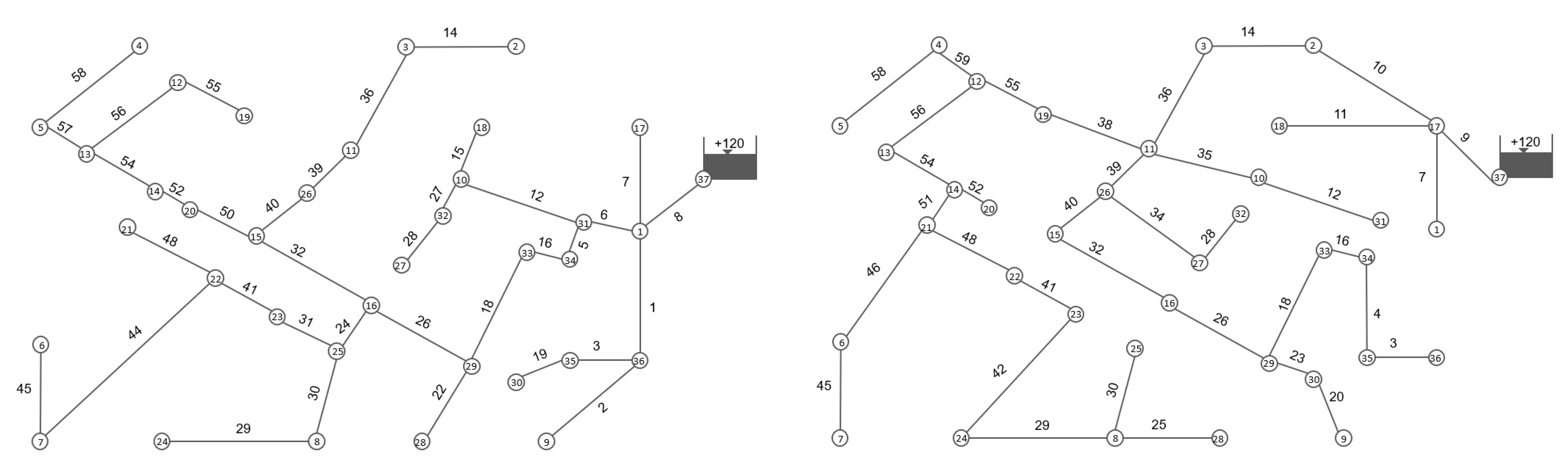
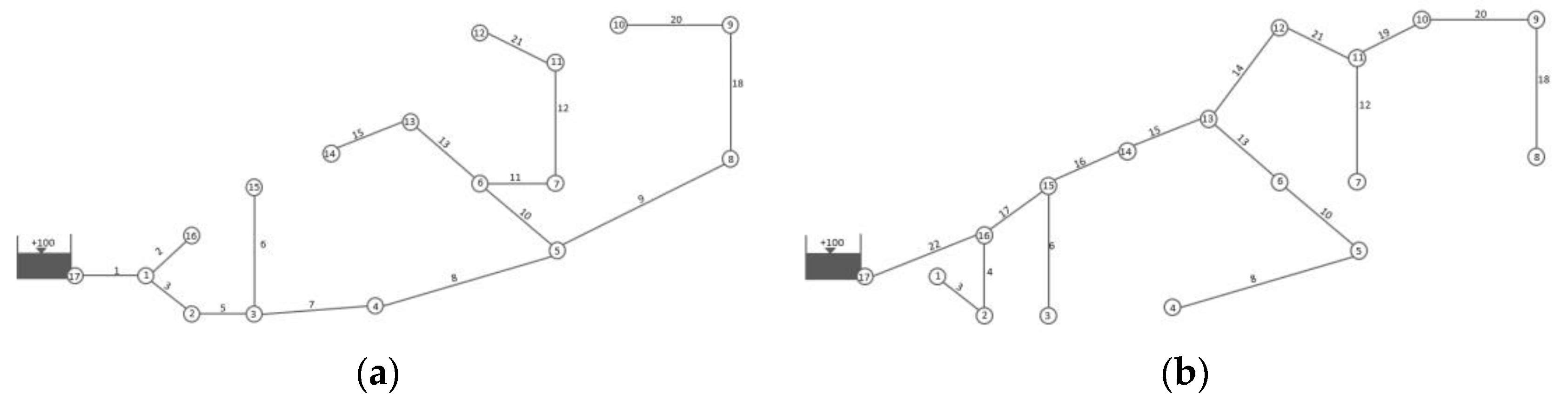
3.1. FOWM Distribution Network

To illustrate the proposed methodology, the Federally Owned Water Main System (FOWM), taken from [1], was examined. Since the network does not satisfy level-1 topology redundancy, five new pipelines are added to convert the layout of the network into a bi-connected graph. The newly added pipelines include edges 〈17,16〉, 〈16,15〉, 〈15,14〉, 〈13,12〉, and 〈11,12〉. Since the network is small, it is possible to scan all possible backup pairs. Figure 1, excluding the source node, is in st numbering.
Seven hundred and sixty-eight backup pairs were scanned for different pressure demands (Figure 2). Component size optimization of any pair was solved using linear programming, where the problem is formulated as cost minimization at each of the required minimum heads, and minimum head requirements for both backups are the constraints.
The backups that give the Pareto front (the lowest cost at every pressure demand) corresponds to the backups with the shortest distance from the source to the demand nodes. However, each node’s demand and elevation values also contribute to the optimal results of the back selection problem. The optimal backup pair is presented in Figure 3.

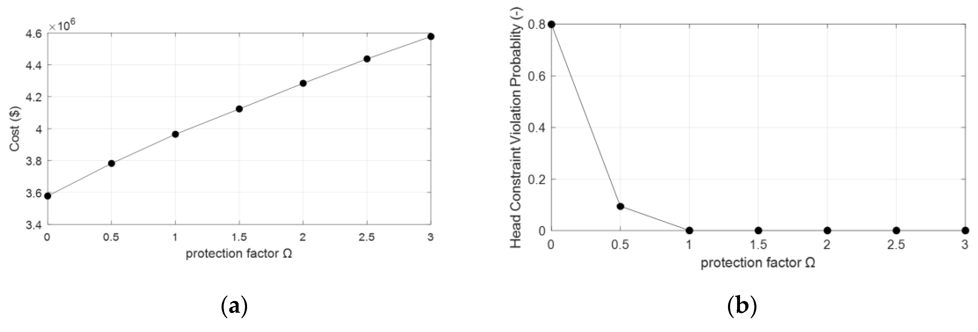
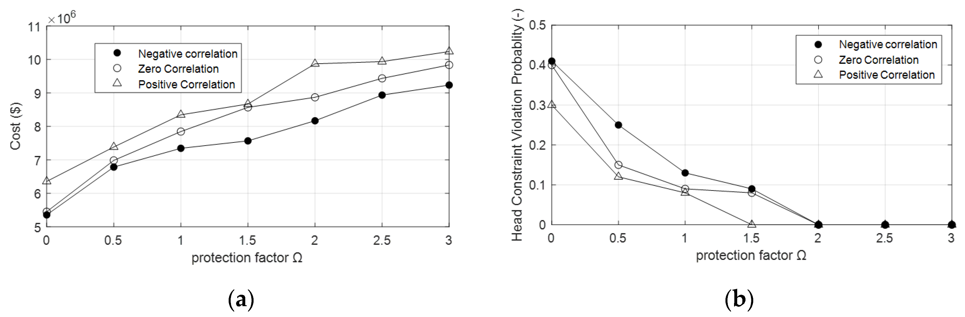
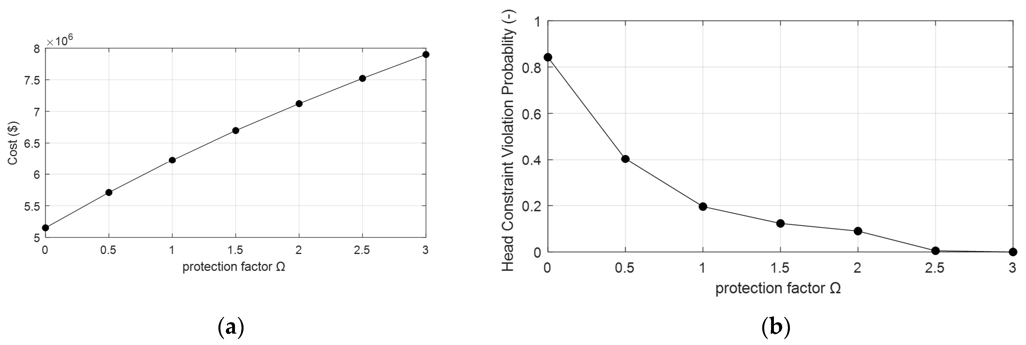
3.1.1. Uncorrelated Data Uncertainty

The uncorrelated consumer demand data uncertainty model assumes demand uncertainty affects the linear mass balance constraint. The new problem resembles the original problem with a safety factor accounting for the standard variation of the demand and the size of the uncertainty space considered. Since the backups are tree networks whose flows are readily known, the cost minimization problem was solved using linear programming accounting for head constraints for both backups. In the absence of actual data for the network under consideration, random standard deviation values up to 50% of the expected demand were generated to calculate the standard deviation of the consumer demand for the networks. The safety factor values taken in this study are ω = {0, 0.5, 1, 1.5, 2, 2.5, 3}.
The cost vs. safety factor graph shown in Figure 4a indicates that the cost increases as the value of the safety factor increases. This can be seen from the mass balance equation in which the effective demand for which the network is being designed increases as the safety factor increases.
In order to examine a sensitivity analysis on minimum head requirement violation for the uncorrelated model, 1000 Monte Carlo simulation was conducted for each safety factor. The sampling was carried out on q [ q ˜ δ , q ˜ + δ ] , assuming the demand q is uniformly distributed over the given range. The result depicted in Figure 4b indicates as the safety factor increases, the probability of minimum head violation decreases. When the safety factor ω ≥ 1, the probability of head constraint violation becomes 0 since the effective demand for which the network is being designed now exceeds the maximum demand.

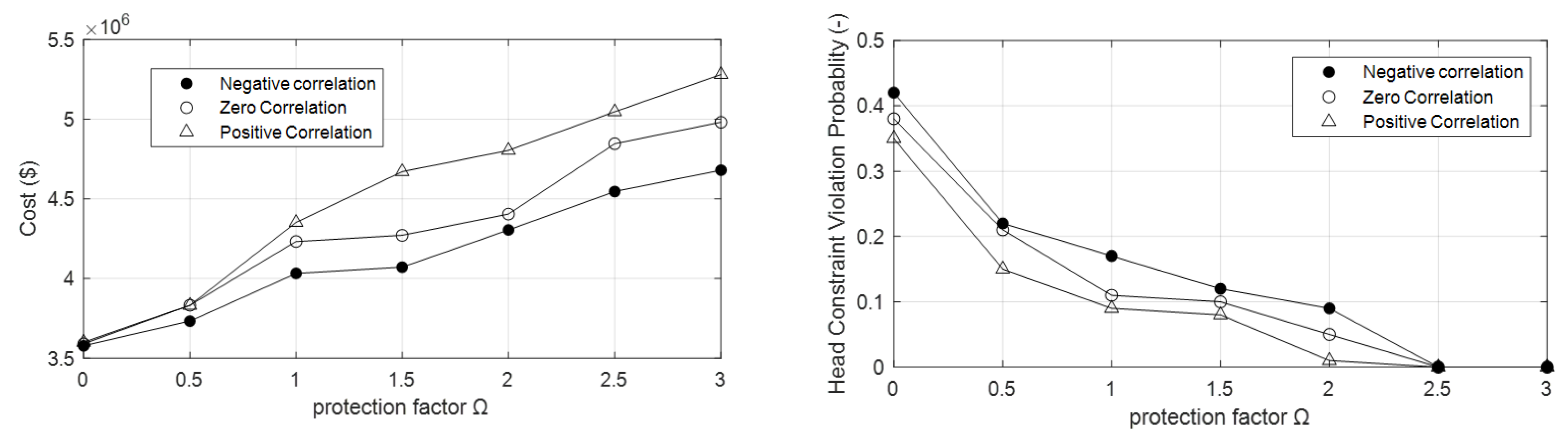
3.1.2. Correlated Data Uncertainty

In this uncertainty data model, two of the drawbacks of the first model were solved. The first drawback in the uncorrelated data model was that the effect of uncertainty in demand on minimum head constraint was not accounted. Additionally, the second was that the correlation between demand nodes was not addressed.
Although the backups are tree networks, the problem is no longer linear due to the nonlinearity of the new constraint obtained from the robust counterpart. The optimization problem was solved using a genetic algorithm. In this problem, the genetic algorithm is coded in binary, where 4 digits of 0 and 1 bits are used to represent the commercially available diameters. The parameters of the ga algorithm were as follows: Maximum generation = 10,000, population size = 100, mutation rate = 0.05, and two-point crossover mechanism with 0.9 crossover probability.
The correlation matrix is assumed to be a function of demand standard deviation and correlation sign represented by ρ . The robust design for the correlated data uncertainty was examined for three types of correlation :   ρ = [ 0.9 ,   0 ,   0.9 ] , representing negative, zero, and positive correlations, respectively. In addition, a Monte Carlo simulation was conducted for all three correlations, and the result is depicted in Figure 5.

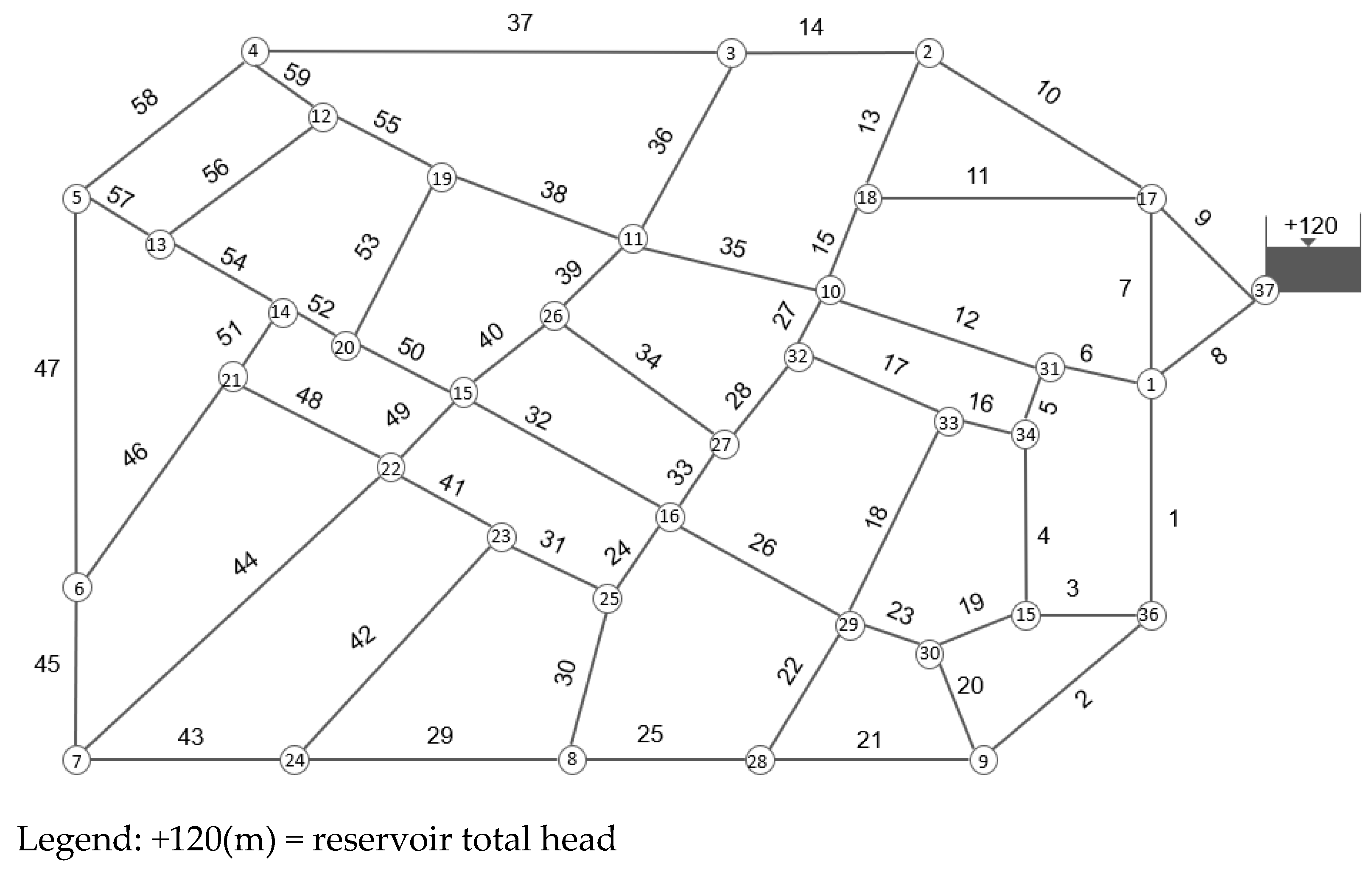
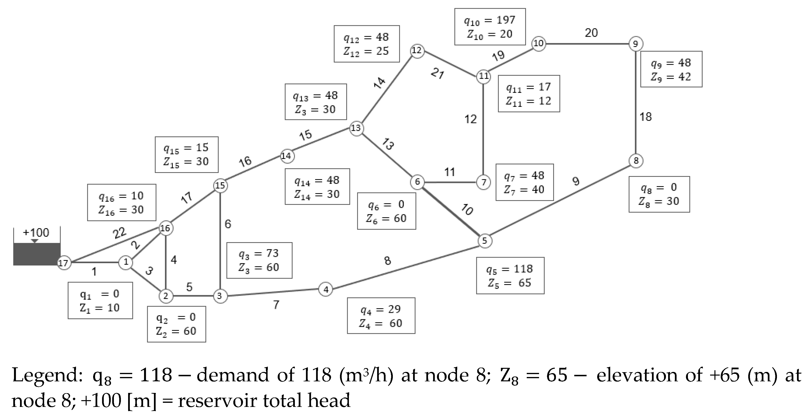
3.2. Fossolo Distribution Network

The Fossolo system (Figure 6) is based on the water distribution system for the neighborhood of Fossolo in Bologna, Italy. It has an average demand of 3000 cubic meters per day and consists of a single reservoir as a source node. The Fossolo network has been used as an example network in various water distribution network studies. Since the original network does not satisfy level-1 redundancy from a topology point of view, one pipe that connects the source with node 17 was added.
Since the number of possible backup pairs is significantly large, scanning all possible candidate pairs is difficult. Thus, a heuristic search is needed to find the backup pairs that yield the Pareto optimal front, whereas linear programming is sufficient for pipe size optimization for each backup pair. The cost vs. minimum pressure curve and the optimal pair of the subsystem are shown in Figure 7 and Figure 8, respectively.
The results in Figure 7 shows a tradeoff between investment cost and required minimum pressure for the backups. In addition, it can be seen how the genetic algorithm improves the backup selection. Similar to the first example network, the backups that yielded the Pareto front (lowest cost at every pressure demand) correspond to the backups with the shortest distance from source to the demand nodes. However, the nodes with a high load (i.e., high demand and elevation) also contribute to the backup selection.

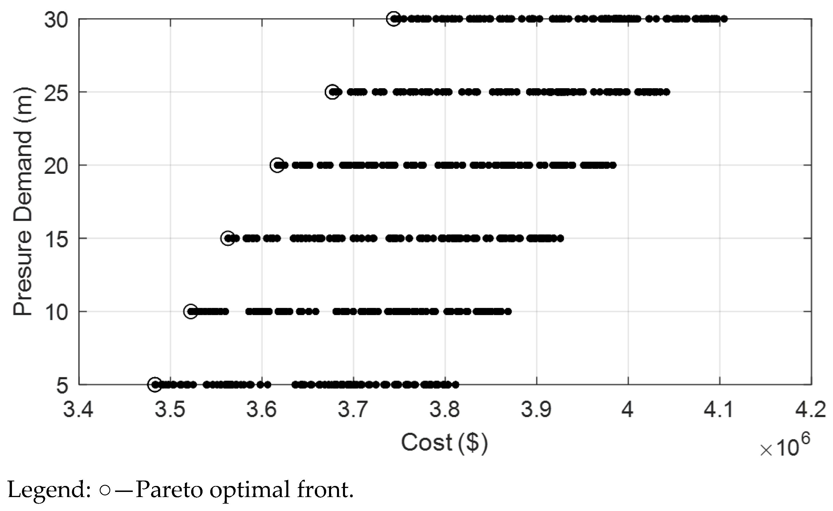
3.2.1. Uncorrelated Data Model

According to the uncorrelated consumer demand data uncertainty model, demand uncertainty affects the linear mass balance constraint (Kirchhoff’s first law) while its influence on energy balance is disregarded. The deterministic equivalence problem is linear; therefore, linear programming is sufficient to solve it. In order to examine a sensitivity analysis on minimum head requirement violation for the uncorrelated model, 1000 Monte Carlo simulation was conducted for each safety factor. The sampling was carried out on q [ q ˜ δ ,   q ˜ + δ ] .   The demand q is assumed to be normally distributed over the given range.
Figure 9 contains cost vs. safety factor and sensitivity analysis for the uncorrelated case.

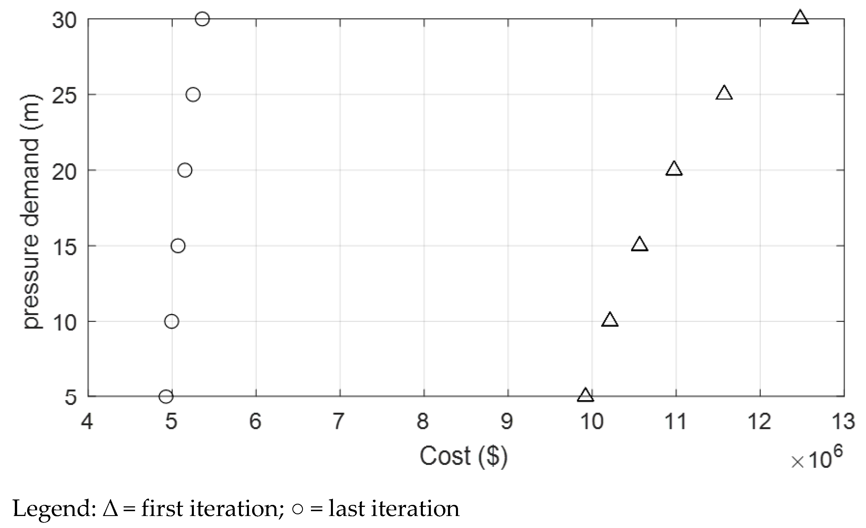
3.2.2. Correlated Data Uncertainty

This uncertainty data model resolves two of the shortcomings of the first model. The first issue with uncorrelated data models was that the effect of uncertainty in demand on the minimum head constraint was not taken into consideration. Second, there was no consideration given to the correlation between demand nodes. Even though the backups are tree networks, the problem is no longer linear due to the nonlinearity of the new constraint derived from the robust counterpart. Due to this reason, a genetic algorithm was employed to solve the optimization problem. The ga parameters are the same for both networks. Figure 10a shows cost vs. protection factor for the correlated data uncertainty model.
The head constraint violation sensitivity analysis (Figure 10b) was performed by conducting 1000 Monte Carlo simulations. The uncertain parameter q is assumed to be normally distributed with an average value of     q ˜ , and standard deviation of δ . According to the results, the probability of minimum head violation is generally low in the correlated data uncertainty model compared to the uncorrelated model, showing the result of the correlated model for the negative correlation. As the safety factor increases, a proportional increment in costs is observed.

4. Discussion

Generally, the uncorrelated data model is conservative since the correlation between demand nodes and uncertainty propagation to the energy balance constraint are ignored. There is a significant reduction in system reliability for the uncorrelated data model in the low region of the protection factor, as shown in the results section. In addition, the price of robustness for three of the correlation types (negative, zero, and positive) varies. According to the results, the cost of design increases as the protection factor increases, while the probability of head constraint violations decreases. Additionally, as expected, the costs of the designs for negative correlation are lower than for zero correlation, and these are, in turn, lower than for positive correlation. This is because the correlation between node demands is a measure of how demand variation at each node is related. A positive correlation means the nodes are simultaneously at their maximum/minimum demand. A negative correlation means that when one node is at its maximum, the other is towards its minimum value. Therefore, designing a network with demand values that tend to vary in a similar manner is more expensive than those that vary differently.

5. Conclusions

This research indicates that subsystem networks with reliability represented in terms of explicit redundancy level can be used for WDS optimization, and performance can be further enhanced with the inclusion of uncertainty in some of the design parameters. It can be also inferred that the subsystem selection problem for the subsystem-based two stage approach should be treated as an optimization problem and robust solutions obtained from robust optimization. The results show that a selection of backup pairs influences the optimal outcome; therefore, it should be considered during problem optimization. It appears that previous efforts, which are mainly based on the shortest path method to select subsystem pairs, are suboptimal since some of the factors that affect the subsystem selection problem are neglected. However, the issue of a system over-redundancy associated with this approach remains unsolved. Therefore, additional research is needed. Further considerations are also required on the service constraint from subsystems and how it is related to the overall optimality.

Author Contributions

Conceptualization, A.H. and A.O.; Methodology, A.H. and A.O.; Writing—Original Draft Preparation, A.H.; Writing—Review and Editing, A.H. and A.O.; Supervision, A.O.; Project Administration, A.O.; Funding Acquisition, A.O. All authors have read and agreed to the published version of the manuscript.

Funding

This research received no external funding.

Institutional Review Board Statement

Not applicable.

Informed Consent Statement

Not applicable.

Data Availability Statement

The data presented in this study are available on request from the corresponding author.

Conflicts of Interest

The authors declare no conflict of interest. The funders had no role in the design of the study; in the collection, analyses, or interpretation of data; in the writing of the manuscript, or in the decision to publish the results.

Appendix A. Solution to a Subproblem

Minimize c T x   s . t a ( ξ ) T   x b ,           ξ U
Box model:  U = { ξ | ξ r }
max ξ U (   ξ T diag ( a ˜ ) x ) + a 0 T   x b 0
where d i a g ( a ˜ ) refers to a diagonal matrix with its diagonal entry   a ˜ .
If there is more than one constraint in the original problem, it needs to be written explicitly for each constraint and solve the problem of max ξ U ( ξ T d i a g ( a ˜ ) x ) . Since b   and a 0 are not dependent on ξ , they can be taken out of the optimization. It can be seen that the remaining problem is simply a dot product between vectors ξ and d i a g ( a ˜ ) x .
The supremum value of ξ T d i a g ( a ˜ ) x can be achieved using Holder’s inequality. Holder’s inequality relates the norm of two vectors f and g to their dot product value as stated below
| f T g | f p   g q   1 p + 1 q = 1
When p = q = 2, a very special case of Holder’s inequality which is called Cauchy–Schwarz inequality is achieved. Using the fact that a dot product of two vectors cannot be greater than its absolute value, choosing p = 1 and q = ∞, and combining it with Holder’s inequality, ξ T d i a g ( a ˜   ) x can be bounded from above.
max ξ U (   ξ T diag ( a ˜ ) x ) max ξ U | ξ T diag ( a ˜ ) x | diag ( a ˜ ) x 1 max ξ U | | ξ | | = diag ( a ˜ ) x 1   r
The last equality is obtained from the fact that max ξ U ξ = r . The supremum value is attained when ξ i = r a ˜ i   x i | a ˜ i x i | , which satisfies the constraint ξ U = ξ r . The worst realization constraint now becomes:
r diag ( a ˜ ) x 1 + a 0 x b 0  
An alternative way to solve the subproblem is by adding a Lagrangian multiplier and thus converting the problem from constrained to unconstrained optimization problem.
Finally, the deterministic equivalent for cube uncertainty space is
Minimize c T x s . t r diag ( a ˜ ) x + a 0 x b 0
Although the problem is now no longer linear, it is a convex problem. Therefore, it can be solved using methods available to solve convex optimization problems.
Ellipsoidal set:
U = { a ( a a ˜ ) T   Σ 1   ( a a ˜ ) ω 2   }
By making a variable transformation of Σ = P P T   a n d   a = a ˜ + P ξ , the uncertainty space becomes
U = { a a = a ˜ + P ξ , ξ ω }
Note that a very special case of an ellipsoidal uncertainty set is a spherical space. In the same way the box set is defined, the worst-case realization can be formulated, and the subproblem can be thus optimized over the ellipsoidal space.
Minimize c T x s . t max ξ U ( ( a ˜ + P ξ ) T x b ) 0
By solving max ξ U ( ( a ˜ + P ξ ) ^ T   x b ) , the worst scenario can be obtained. Again, it can be shown that the maximum is ω P T x and it is attained when ξ = ω P T x P T x , which also satisfies the constraint ξ = ω P T x P T x = ω P T x P T x = ω ω .
The robust deterministic equivalent for ellipsoidal uncertainty is:
Minimize c T x   s . t a ˜ T x + ω P T x b 0
Therefore, robust optimal solutions can be achieved by solving the robust deterministic equivalent written in Equation (A10).

References

  1. Ormsbee, L.; Kessler, A. Optimal upgrading of hydraulic-network reliability. J. Water Resour. Plan. Manag. 1991, 116, 784–802. [Google Scholar] [CrossRef]
  2. Agrawal, M.L.; Gupta, R.; Bhave, P.R. Optimal Design of Level 1 Redundant Water Distribution Networks Considering Nodal Storage. J. Environ. Eng. 2007, 133, 319–330. [Google Scholar] [CrossRef]
  3. Rathi, S.; Gupta, R. Genetic Algorithm for Minimization of Variance of Pipe Flow-Series for Looped Water Distribution Networks. In Hydrological Modeling; Springer: Cham, Switzerland, 2022; pp. 205–219. [Google Scholar] [CrossRef]
  4. Yazdani, A.; Jeffrey, P. Applying Network Theory to Quantify the Redundancy and Structural Robustness of Water Distribution Systems. J. Water Resour. Plan Manag. 2012, 138, 153–161. [Google Scholar] [CrossRef]
  5. Rathi, S.; Gupta, R.; Palod, N.; Ormsbee, L. Minimizing the variance of flow series using a genetic algorithm for reliability-based design of looped water distribution networks. Eng. Optim. 2020, 52, 637–651. [Google Scholar] [CrossRef]
  6. Gupta, R.; Kakwani, N.; Ormsbee, L. Optimal Upgrading of Water Distribution Network Redundancy. J. Water Resour. Plan Manag. 2015, 141, 04014043. [Google Scholar] [CrossRef]
  7. Jung, D.; Kim, J.H. Water distribution system design to minimize costs and maximize topological and hydraulic reliability. J. Water Resour. Plan Manag. 2018, 144, 06018005. [Google Scholar] [CrossRef]
  8. Ostfeld, A.; Shamir, U. Design of optimal reliable multiquality water-supply systems. J. Water Resour. Plan. Manag. 1996, 122, 322–333. [Google Scholar] [CrossRef]
  9. Filion, Y.R.; Adams, B.J.; Karney, B.W. Stochastic design of water distribution systems with expected annual damages. J. Water Resour. Plan Manag. 2007, 133, 244–252. [Google Scholar] [CrossRef] [Green Version]
  10. Kapelan, Z.; Babayan, A.V.; Savic, D.A.; Walters, G.A.; Khu, S.T. Two new approaches for the stochastic least cost design of water distribution systems. Water Sci. Technol. Water Supply 2004, 4, 355–363. [Google Scholar] [CrossRef]
  11. Guistolisi, O.; Laucelli, D.; Colombo, A.F. Deterministic versus stochastic design of water distribution networks. J. Water Resour. Plan Manag. 2009, 135, 117–127. [Google Scholar] [CrossRef]
  12. Ben-Tal, A.; El Ghaoui, L.; Nemirovski, A. Robust Optimization; Princeton University Press: Princeton, NJ, USA, 2009. [Google Scholar] [CrossRef]
  13. Perelman, L.; Housh, M.; Ostfeld, A. Robust optimization for water distribution systems least cost design. Water Resour. Res. 2013, 49, 6795–6809. [Google Scholar] [CrossRef]
  14. Perelman, L.; Housh, M.; Ostfeld, A. Explicit demand uncertainty formulation for robust design of water distribution systems. In Proceedings of the World Environmental and Water Resources Congress 2013: Showcasing the Future, Cincinnati, OH, USA, 19–23 May 2013; pp. 684–695. [Google Scholar] [CrossRef]
  15. Itai, A.; Rodeh, M. Multi-Tree Approach To Reliability in Distributed Networks. Annu. Symp. Comput. Sci. 1984, 79, 43–59. [Google Scholar]
  16. Takeaki, U.N.O. An algorithm for enumerating all directed spanning trees in a directed graph. In International Symposium on Algorithms and Computation; Lect Notes Comput Sci (Including Subser Lect Notes Artif Intell Lect Notes Bioinformatics); Springer: Berlin/Heidelberg, Germany, 1996; Volume 1178, pp. 167–173. [Google Scholar] [CrossRef]
  17. Geen, Z.W. Multiobjective Optimization of Water Distribution Networks Using Fuzzy Theory and Harmony Search. Water 2015, 7, 3613–3625. [Google Scholar] [CrossRef]
Figure 1. Network schematic of FOWM distribution system (Ormsbee and Kessler 1990).
Water 14 02443 g001
Figure 2. Cost vs. minimum pressure demand for FOWM network.
Water 14 02443 g002
Figure 3. Schematic of pair of backups: (a) The first subsystem generated following decreasing order; (b) The second subsystem generated following increasing order.
Water 14 02443 g003
Figure 4. Results of uncorrelated optimization for FOWM network: (a) cost vs. protection factor Ω; (b) head constraint violation probability.
Water 14 02443 g004
Figure 5. Results of correlated optimization for FOWM network.
Water 14 02443 g005
Figure 6. Network schematic of Fossolo distribution system.
Water 14 02443 g006
Figure 7. Cost vs. minimum pressure-demand tradeoff curve for Fossolo network.
Water 14 02443 g007
Figure 8. Schematic of pair of optimal backup pairs for Fossolo network.
Water 14 02443 g008
Figure 9. Results of uncorrelated optimization for Fossolo network: (a) cost vs. protection factor Ω; (b) head constraint violation probability.
Water 14 02443 g009
Figure 10. Results of correlated optimization for Fossolo network: (a) cost vs. protection factor Ω; (b) head constraint violation probability.
Water 14 02443 g010
Publisher’s Note: MDPI stays neutral with regard to jurisdictional claims in published maps and institutional affiliations.

