1. Introduction
Water hammer models are becoming more present in designing and analyzing complex pipeline systems. In addition, they are more frequently used for the identification of system leakage, closed or partially closed valves, and the assessment of water quality problems. Traditionally, steady or quasi-steady friction terms are incorporated into standard water hammer algorithms. This assumption holds for slow transients in which the wall shear stress behaves similarly to a quasi-steady force. Previous experimental validations of steady friction models for rapid transients revealed significant differences in attenuation and phase shift of pressure traces when the computed results are compared with the measured results. Turbulence models have been developed and used to perform numerical experiments in turbulent water hammer flows for a multitude of research purposes, such as the computation of instantaneous velocity profiles and shear stress fields, the calibration and verification of water hammer models, the evaluation of the parameters of unsteady friction models, and the comparison of various unsteady friction models.
Understanding the governing equations that are in use in water hammer research and practice and their limitations is essential for interpreting the results of the numerical models that are based on these equations, judging the reliability of the data obtained from these models, and minimizing misuse of water hammer models. While the most common approaches used to describe transient events in the literature are inherently Eulerian, they require a dense mesh to mimic real-life transient events and guarantee accurate results. Subsequently, significantly increasing the computational capacity, time and resources required. Consequently, deeming these models impractical to use in advanced optimizing algorithms. For instance, stochastic algorithms (e.g., genetic algorithms) are inconvenient to work with when dealing with time extensive simulation, since their efficiency relies on the parallel speed of the simulation.
While advanced sophisticated methods attempt to mathematically describe and model the shear stresses and velocity profiles to better mimic transient events in a lab, it can lead to misuse and inaccurate estimation in real-life settings. Therefore, the suggested method attempts to capture the transient behavior by introducing a calibrated factor that can accommodate the unknown uncounted-for parameters that exist in real-life networks.
This work presents a framework for simulating the head-damping effect in transient flows when modeled in the Lagrangian approach. The Lagrangian approach normally requires orders of magnitude fewer calculations, which allows very large systems to be solved in an expeditious manner, and it has the additional advantage of using a simple physical model as the basis for its development. Moreover, since it is continuous in both time and space, the method is less sensitive to the structure of the network and the length of the simulation process, resulting in improved computational efficiency. The proposed model relies on the wave characteristics method (WCM) introduced by Wood [
1] and describes a declining wave celerity along with an unsteady friction factor. The celerity is modeled in such that it decreases while the waves propagate through the pipelines due to energy dissipation.
1.1. Models
Unsteady turbulent flows in pipes are described by a system of hyperbolic-parabolic partial differential equations that cannot be solved analytically in most cases. Therefore, numerical solutions are employed to approximate them. The development of theories and models to better characterize and manage hydraulic transients in pipeline systems has been the subject of extensive research. Previous studies have employed one-dimensional models to analyze the efficiency of systems’ transient responses [
2,
3,
4,
5,
6,
7]. Although it cannot accurately depict the system’s transient responses without additional calibrations and tunings, one-dimensional methods are still the most popular method in software used for practical simulations. More recent studies have suggested and explored more complex two-dimensional and quasi-two-dimensional models that can contain various factors [
4,
8]. Numerous methods applied transient analysis to detect various anomalies along the distribution system. For instance, Meniconi et al. [
9] and Chen et al. [
10] developed creative techniques for partial blockage detection in pipeline systems. Other researchers focused on detecting water leakages and assessing pipe conditions using transient analysis. [
11,
12,
13,
14,
15,
16,
17,
18,
19]. Furthermore, it is possible to assess the network layout including pipes, side branch, and dead ends, as demonstrated in the works of Duan and Lee [
20], Kim [
21], and Meniconi et al. [
22].
The understanding of transient flows and transient system responses is crucial to the practical use of transients and the minimization of damage to the physical infrastructure [
2,
3,
23]. Creaco et al. [
24] discussed two demand-modeling methods for investigating extended period simulations coupled with unsteady flow models. Contrary to this study, the unsteady flow modeling method used was an Eulerian approach based on the method of characteristics (MOC) [
25], which was further tested on a laboratory scale. A finite difference method is explained in [
26]. Marsili et al. [
27] proposed a stochastic approach to modeling and analyzing water distribution system transients. Based on the method of characteristics, including unsteady friction, their analysis was verified through laboratory tests.
1.2. Friction Models
Numerous approaches have been developed to numerically model pressure waves in water distribution systems. These approaches may be categorized as either Eulerian or Lagrangian in nature. The Eulerian approach reformulates transient flow equations into total differential equations, which are then expressed as finite differences. Lagrangian theory, on the other hand, tracks pressure changes as they travel through a pipe network and updates the state only when a change occurs. There are many well-known numerical challenges in solving the transient flow equations, including avoiding numerical dispersion and attenuation, and eliminating unnecessary distortion of the physical system or its boundaries.
The development and incorporation of quasi-steady and unsteady friction models into pipeline unsteady flow models has been the subject of many studies. In their 2005 paper, Ghidaoui et al. [
23] observed that steady or quasi-steady friction models are unable to account for the damping of transient pressure found in experimental observations. By contrast, pressure damping is better accounted for by using unsteady friction and turbulence models [
28,
29,
30,
31,
32,
33,
34,
35,
36,
37,
38,
39,
40], which are then validated through experimental measurement under a wide range of flow Reynolds numbers, from laminar to highly turbulent regimes [
41,
42,
43,
44,
45,
46,
47,
48,
49,
50]. Martins et al. [
51,
52] used the CFD approach to simulate and model transient pressure distributions and wall shear stress in pipeline systems. While Ramos et al. [
53] developed a dimensionless form of pressurized transient flow equations to depict surge damping in a single pipe line system. In the work of Wahba [
54], a Runge–Kutta scheme was developed to simulate unsteady flow in elastic pipes due to sudden valve closure.
2. Materials and Methods
In the following description of the model formulation, the WDS mapping is explained as well as the proposed Lagrangian transient modeling, followed by a comparison with the TSNET package developed by Xing and Sela [
55]. Throughout the following sections, the wave characteristic method with quasi-steady friction is referred to as Q-WCM [
56]. The refined wave characteristic method with unsteady friction is referred to as U-WCM, and the TSNET method of characteristic with unsteady friction is referred to as U-MOC [
55].
2.1. Mapping the Water Distribution System
An EPANET (.inp) file was imported to prepare the network for transient simulation. A water distribution system was represented as an undirected graph G = (V, E), whose vertices are the consumers, sources, and valves, whereas the edges are the pipes connecting them. In general, different types of vertices are defined as discontinuities with different coefficients of resistance. MATLAB codes and the TSNET Package in Python were used to perform transient calculations and simulations.
2.2. The Wave Characteristic Method Model
In 1965, Wood [
1] introduced the wave characteristic method (WCM), which is based on the notion that transient pipe flow is caused by pressure waves propagating through the system as a result of disturbances being introduced. Pressure waves are described as rapid changes in pressure that propagate at the speed of sound in a liquid pipe medium. Pressure waves propagate in pressurized water pipes at a speed of approximately 1000 m/s in metallic pipes and about 400 m/s in polymeric pipes [
57,
58]. In the presence of discontinuities, these waves are partially reflected and transmitted through the pipe system.
2.3. Pressure Magnitude
Calculating the magnitude of a pressure wave is conducted by using the Joukowsky equation (Equation (1)) under the assumption of an immediate change in the valve opening. In addition to describing the correlation between pressure change Δ
P and flow change Δ
Q, the Joukowsky equation also lays the foundation for the WCM mathematical model. In order to work with head-pressure units, the Δ
P is replaced by the term
, as shown in Equation (1).
where Δ
P represents the pressure, ∆
H is the change in head pressure, Δ
Q is the change in flow rate,
is the pressure wave’s celerity;
A represents the flow section area,
is the fluid density, and
g is the gravitational acceleration constant.
2.4. Unsteady Friction Attenuation
This section elaborates on the modification that has been proposed to the WCM in order to better capture the transient behavior of WDSs. It builds on the previous work of Zeidan and Ostfeld [
56], which introduced a quasi-steady friction model to the WCM. Furthermore, previous studies have examined the effect of friction (viscous resistance) on the propagation of pressure waves by using the orifice analogy (e.g., [
59]). In this case, the pipe was divided into (n + 1) pipes that were similar in length by adding (n) imaginary friction orifices. A friction orifice was modeled as a square-law orifice with an appropriate orifice coefficient. This took the form of a quadratic correlation between the pressure head ∆H and the flow rate Q, as follows:
The terms A, B, and C represent the coefficients for a general representation of the characteristic equation. The coefficient may be time-dependent but known at every time step. The absolute values of Q were employed to make the resistance term dependent on the flow direction.
Due to its simplicity and ability to produce reasonable agreements with experimental pressure head traces, the Brunone et al. [
60] model has become the most widely used modification in water hammer applications. However, it does not fit the Lagrangian approach for transient modeling. It is simply not possible to utilize Brunone’s model using the Lagrangian approach as it lacks the dense mesh necessary. Consequently, in addition to the Darcy–Weisbach equation, the Daily [
28] empirical correction to the wall shear stress model was adopted here to compute the head-loss and shear stresses along the pipelines. Equation (3) is, therefore, proposed as a hybrid model that combines the Daily model with the instantaneous acceleration-based model (IAB). The wall shear stress is expressed as:
where
is the combined steady and unsteady wall shear stresses,
f is the Darcy–Weisbach coefficient,
V is the flow velocity,
D is the pipe diameter, ∂
V/∂
t is the local instantaneous acceleration, and
is Brunone’s friction coefficient.
The result of including the unsteady shear stress model (Equation (3)) into the square-law orifice analogy (Equation (2)) is described by the following equation:
The value of Brunone’s friction coefficient
is calculated using Vardy’s sheer decay coefficient or calibrated in a lab setting. However, the
values available in the literature are mostly applicable to Eulerian models and are not necessarily compatible with Lagrangian methods. As a means of capturing the head-damping phenomenon observed on laboratory testbeds, a
linear damping is introduced as follows:
where
is a calibrated coefficient and t represents the lifespan of the wave. It is worth noting that the value 0.16 is merely an arbitrary number that was calibrated in the first case study and is by no means restrictive.
When examining the modified instantaneous acceleration-based model (MIAB) which was independently formulated by Pezzinga [
47] and Bergant et al. [
48], we can find that the terms for the wave’s celerity is modified to be:
where
is the modified celerity,
is the wave celerity, and
is Brunone’s coefficient, and the MIAB model is elaborately explained in the work of Vítkovský et al. [
61]. In light of the MIAB celerity modification, a simple linear damping factor is proposed for the wave’s celerity in the Lagrangian model, as described below:
where
t represents the duration of the transient wave and
is a calibrated coefficient.
3. Results
3.1. Case Study 01—Proof of Concept
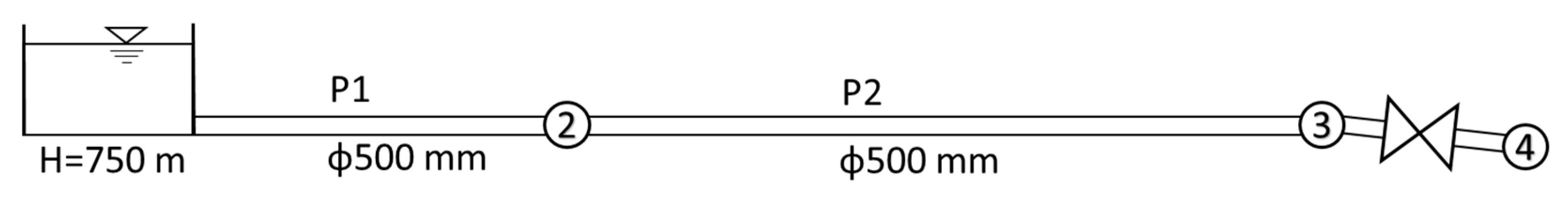
The first network was similar to a simple pipeline system with a valve located downstream. It consisted of a water source at an elevation of 750 m, two steel pipes 500 mm in diameter, and a 50 LPS downhill consumer. The length of pipes (P1) and (P2) were 1.2 km and 2.4 km, respectively. The system’s layout matched the one described in
Figure 1.
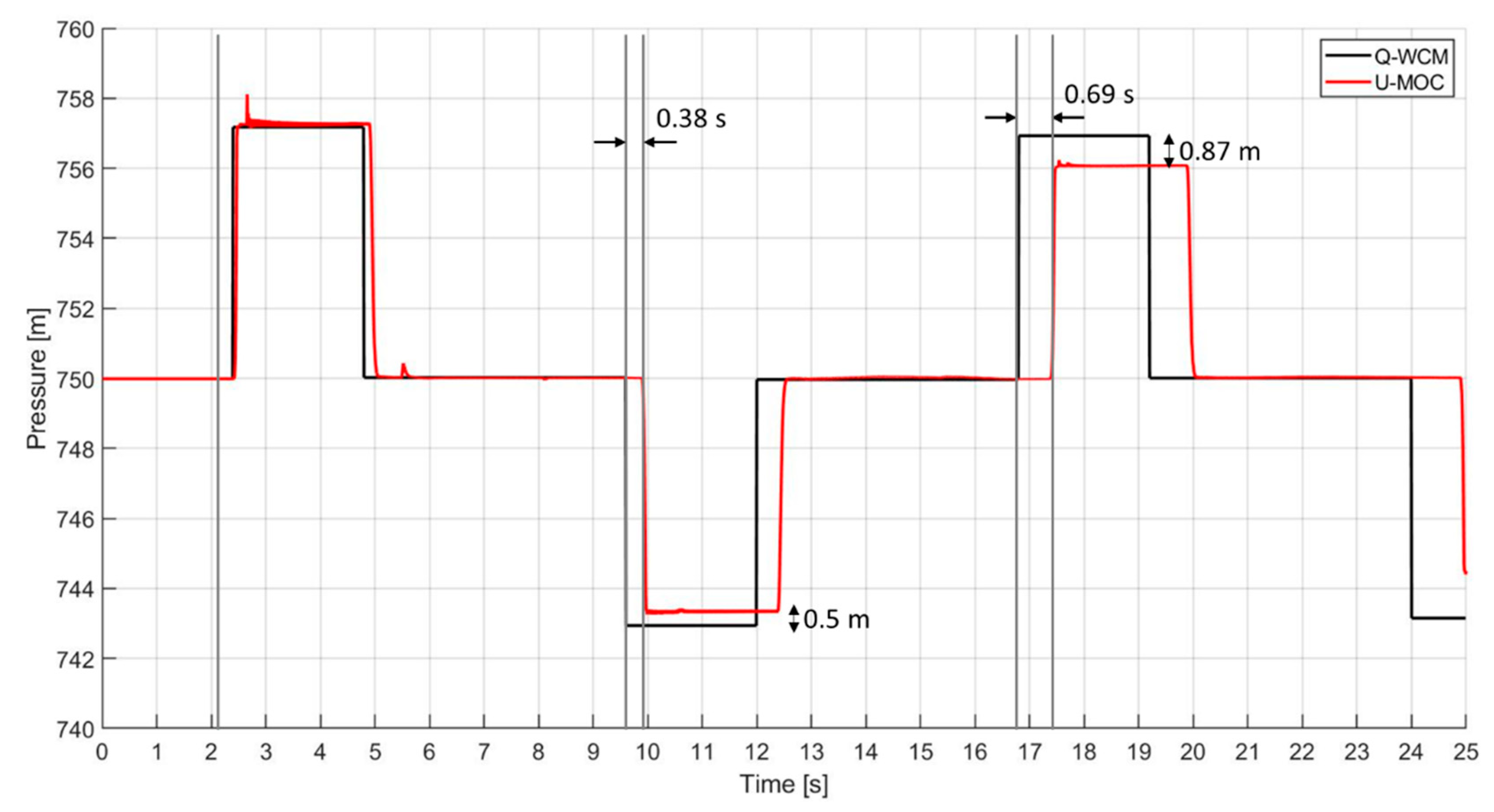
As part of the first case study, the Q-WCM model was compared to the U-MOC model. The main objective of this study was to identify the major differences between the two models as well as the influence of the suggested modification.
Figure 2 shows the pressure fluctuations at node 2 for both models. As is apparent from the graphs, the transient response of the two models differs significantly, with the Q-WCM exhibiting more frequent oscillations and a larger amplitude than its counterpart. Several factors account for this behavior, such as the velocity attenuation and the energy dissipation caused by friction. As time progresses, the velocity of the U-MOC declined, causing the pressure waves to arrive later, while the unsteady friction was responsible for greater head damping.
To evaluate the effectiveness of U-WCM, this case study calibrated and implemented the new suggested parameters (α, β). On the basis of the calibrated parameters, various variations of case study 01 were tested to examine the influence of different network parameters on the transient behavior of the network. It is desirable to obtain constant parameters that will fit into other layouts and will be considered constant coefficients in the future.
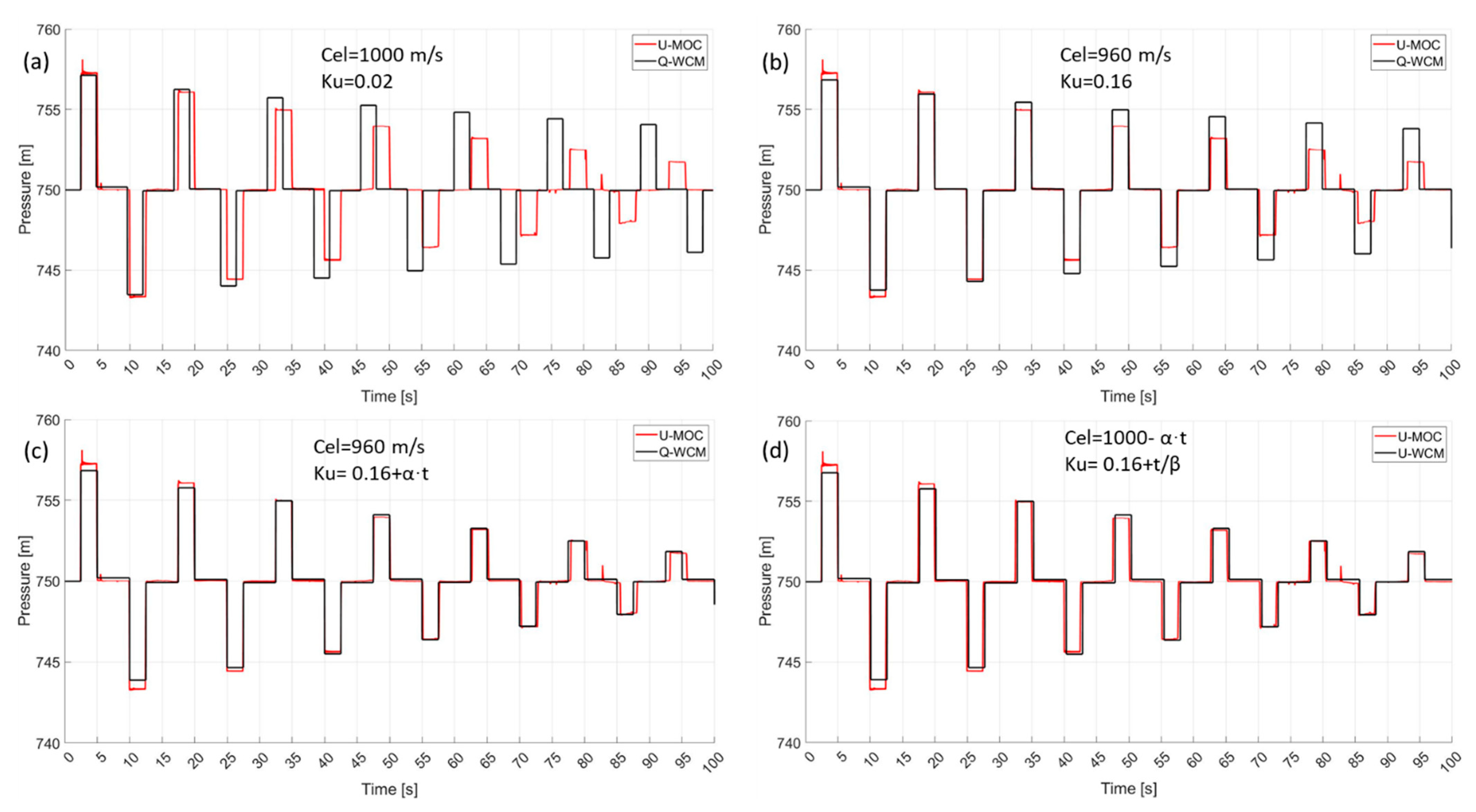
After introducing both the celerity and friction tunings to the Lagrangian model, it was beneficial to observe the influence of each parameter on the transient response. In this case study, the parameters α and β were calibrated to be 0.5 and 150, respectively.
Figure 3 presents the pressure oscillation at node 2 for different tunings. The transient response shown in
Figure 3a served as a baseline for these modifications since it was free of any celerity or friction adjustments.
Figure 3a illustrates that the WCM pulses arrived much faster (with an increasing gape) than their counterparts in the unsteady model, largely due to differences in pressure wave celerity. By adjusting the wave velocity to 960 m/s and the Ku to 0.16, the phase difference was greatly reduced (
Figure 3b); however, the amplitudes were still off. Based on
Figure 3c, it can be observed that by introducing the linear damping effect for the friction factor, both models provided similar transient responses. Finally,
Figure 3d illustrates the impact of adjusting both the celerity and friction factor, where the transient response of U-WCM is remarkably similar to that of U-MOC.
3.2. Sensitivity Analysis
In pursuance of avoiding overfitting and specific sole solutions, the parameters were tested in modified variations of case study 01, where the pipe lengths were altered, but the parameters had not been re-calibrated. The purpose of this study was to examine the transient response for a similar layout with different hydraulics, and assess how the pipe lengths affect the transient response.
Variation A: In the first case study layout, the lengths of the pipes were altered in order to test the calibrated parameters, where the transient response at node number 2 was observed and compared to the U-MOC. The pipe lengths P1 and P2 were changed to 1.5 km and 2.0 km, respectively.
Figure 4 illustrates the transient response of the U-WCM and the U-MOC at node number 2.
As shown in
Figure 4, the transient responses for the two models were fairly similar, with relatively few anomalies. It was found that the retrieved pressure signal from the U-WCM was slightly shifted, and the amplitudes were slightly off by less than one meter in head pressure. However, the differences are negligible from an engineering standpoint, particularly when dealing with such phenomena in an area where background noises and disturbances are prevalent.
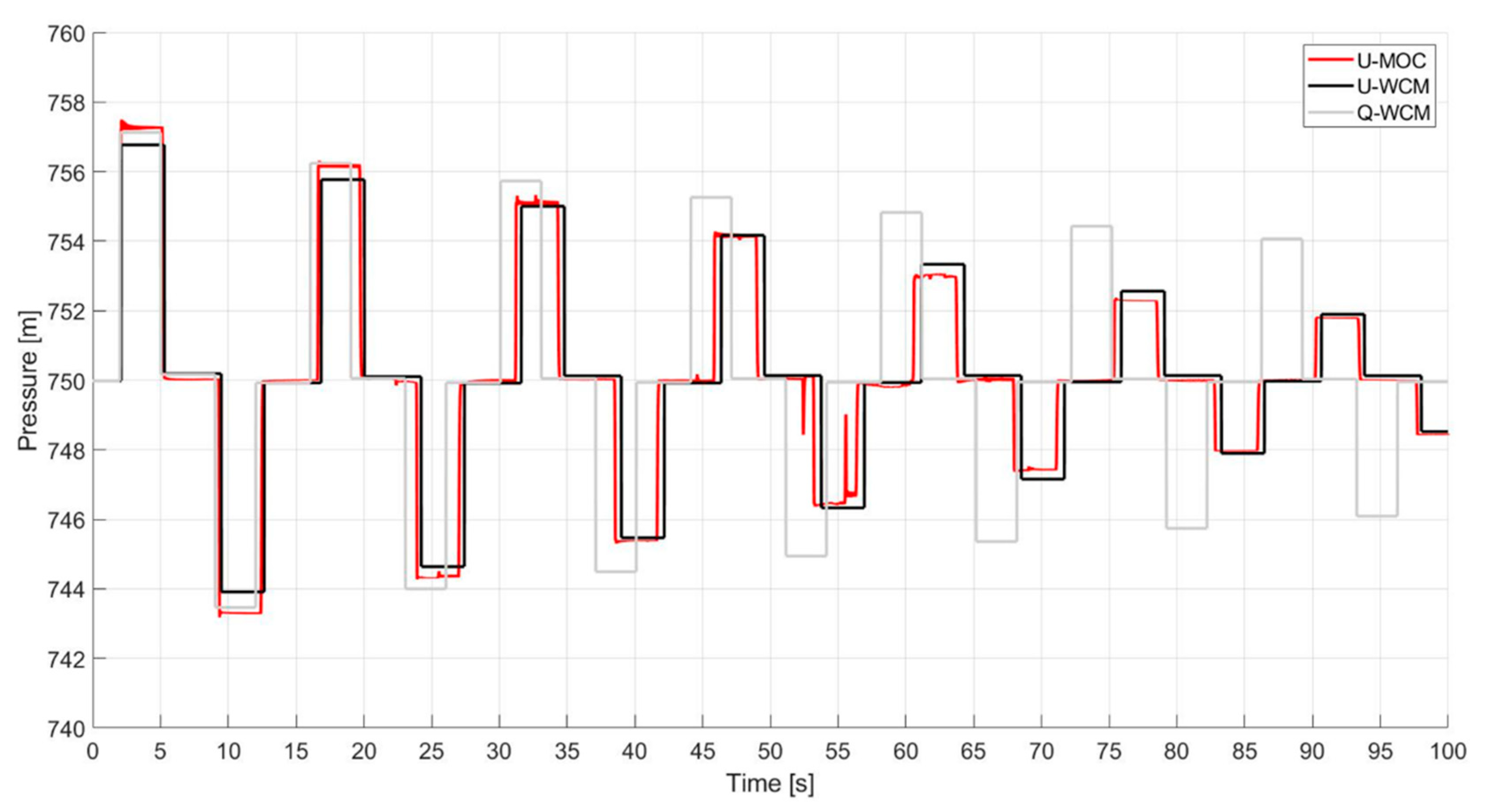
Variation B: The parameters were further tested using a similar layout but with different pipe lengths, where P1 and P2 were each 3.0 km long in this instance.
Figure 5 displays the transient responses of the three models at node number 2.
Based on
Figure 5, the U-WCM can depict a similar transient response to that of the U-MOC; however, it is important to keep in mind that the WCM requires fewer computational resources, thus, requiring less computation time. The U-WCM outperformed the Q-WCM significantly without increasing computational time.
It appears that the U-MOC model performed abnormally around the 75 s mark and forward, and the pressure signal experienced some instability. In this case, it is speculated that the aberrations result from mesh and boundary condition sensitivity. Nonetheless, the U-WCM did not encounter such deviations due to its inherent ‘naive’ Lagrangian approach. A good practice is to carefully modify the mesh and boundary conditions in order to avoid such anomalies. Furthermore, it is important to observe that numerical instabilities are present in Lagrangian methods as well, if they are defined incorrectly.
3.3. Case Study 02—Looped Water System
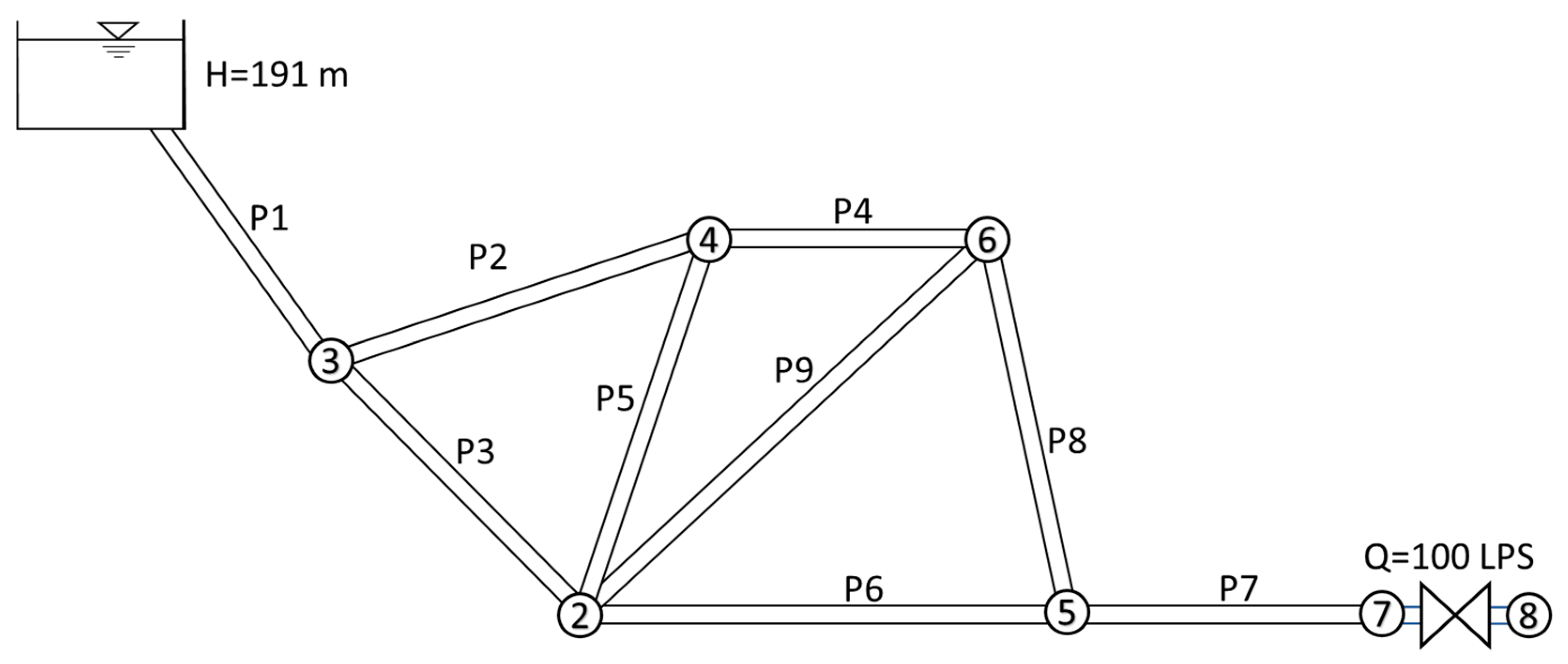
The second network resembles a more complex pipeline system featuring four loops and a valve at the downstream. There was one source of water at an altitude of 191 m, nine steel pipes of varying properties, and a 100 LPS downhill consumer.
Table 1 lists the length and diameter of the pipes. The layout of the system is shown in
Figure 6.
Similar to the first case study, the introduced parameters (α, β) were calibrated to produce a U-WCM transient response that was similar to the U-MOC. Calibration was carried out in a systematic manner and resulted in values of (α = 0.2, β = 100). In the second case study, these values were tested at different nodes to determine whether they are accurate for a particular node or whether they are appropriate for the entire network.
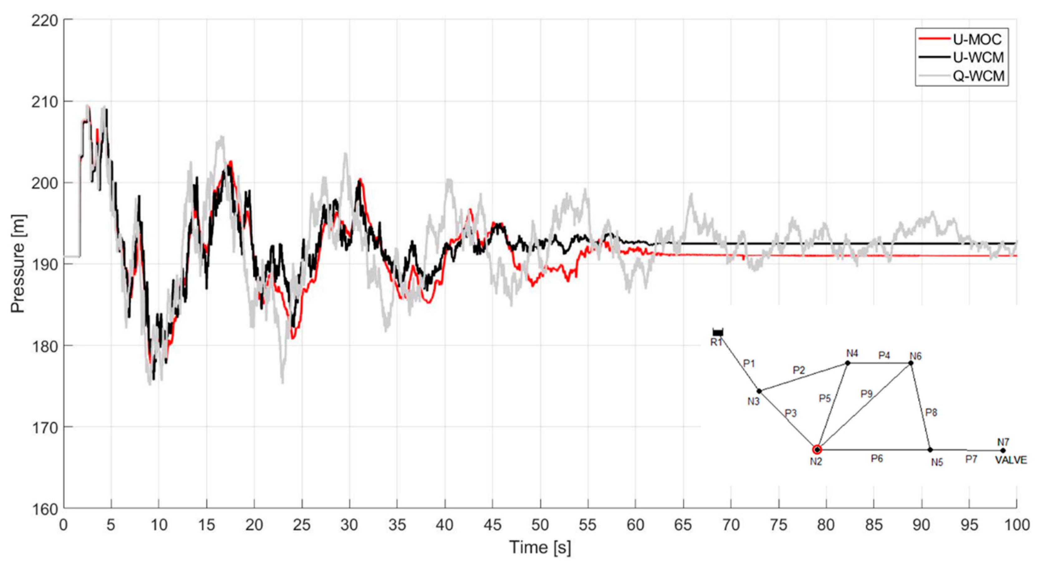
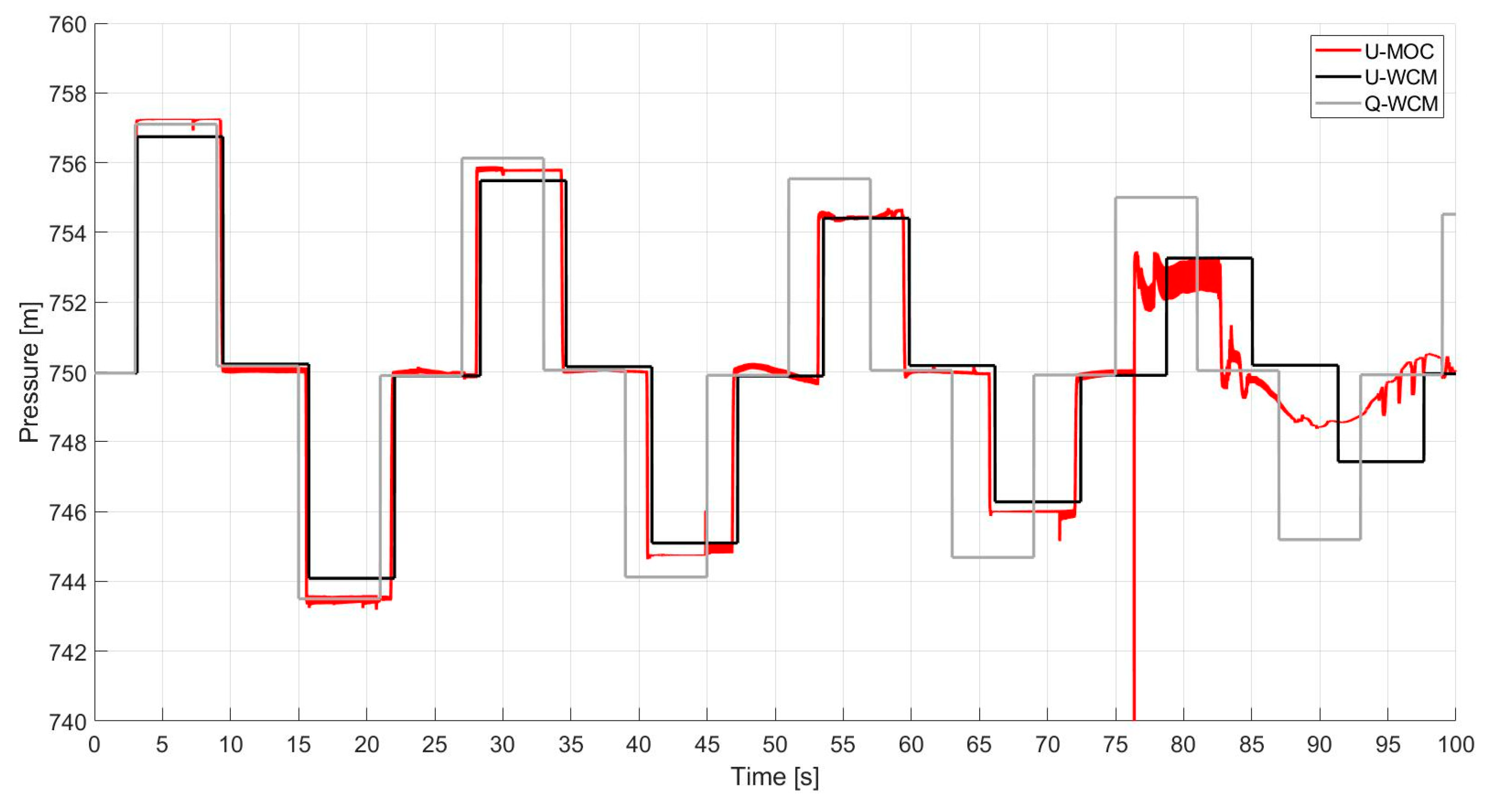
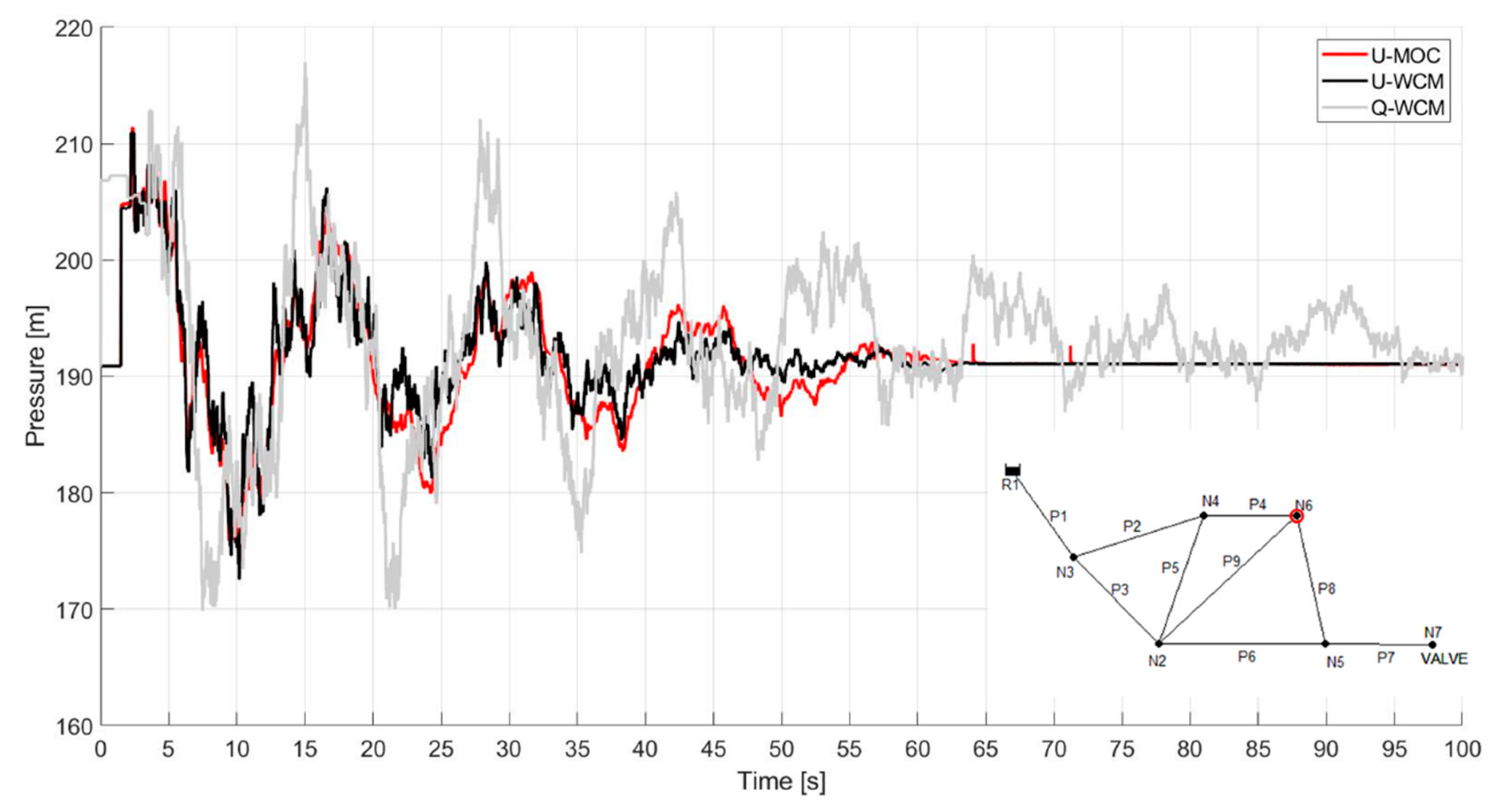
Figure 7 illustrates the pressure oscillation at node 6 in the second case study. The responses of the different models Q-WCM, U-WCM, and U-MOC are shown in gray, black, and red, respectively. Note that the values of α and β in this case study differ from those in the first case study. In addition, the U-WCM shares striking similarities with the U-MOC transient response, while the unmodified Q-WCM model lags behind in terms of both amplitude and celerity. The unmodified Q-WCM model depicts a more powerful and faster pressure wave that dissipates significantly slower than its counterpart. In the U-WCM model, for instance, the pressure oscillation decreases around the 60-s tick mark, whereas the Q-WCM model predicts pressure fluctuations of 10 m.
In this instance, the same parameter values (α = 0.2, β = 100) were tested for a different node (node 2). It is important to emphasize that these parameters were calibrated specifically for node 6.
Figure 8 illustrates the transient response for the three models examined, using colors consistent with the previous graphs. In general, the U-WCM performed well until the 47 s mark, where it experienced slightly higher pressures than the U-MOC. Nevertheless, its advantages are again evident over the unmodified Q-WCM model.
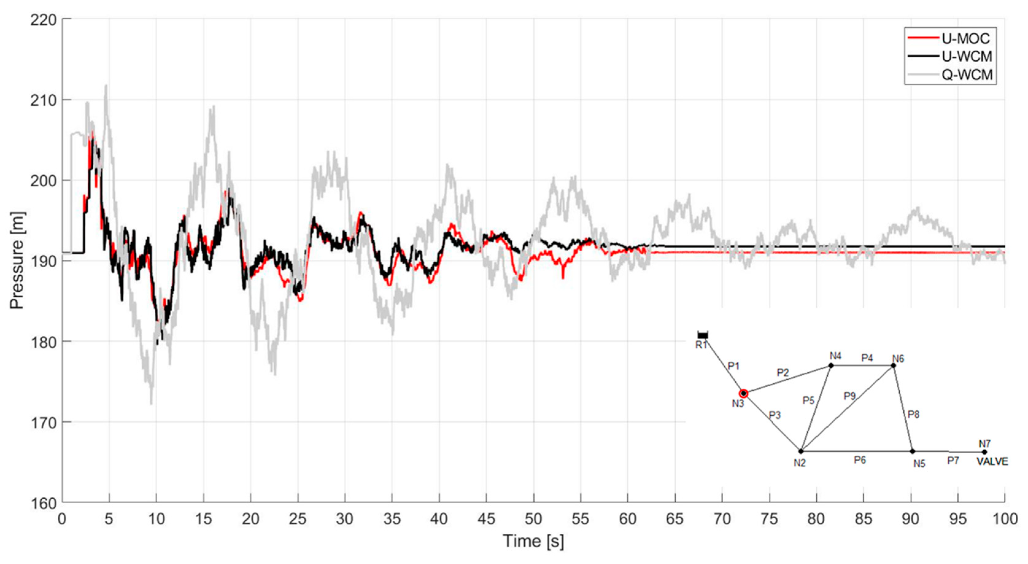
Using the same parameters (α = 0.2, β = 100), a third node (node 3) is tested. It was located much further from the source of the transient wave and close to the water source, which acted as a reflecting boundary condition. It is interesting to examine the behavior of the pressure fluctuations in the vicinity of the water source.
Figure 9 illustrates the transient response for the three models examined in colors consistent with those of the previous graph. The U-WCM performance is much better than that of the last example, and it correlates well with the U-MOC and has a clear advantage over the Q-WCM. Therefore, it is safe to assume that the suggested U-WCM model holds a higher potential in representing the transient behavior than the quasi model.
4. Conclusions
In previous studies, numerous models have been developed for simulating transient responses which capture the damping effect experienced in more realistic laboratory settings. However, the majority of these models included a modification based on an Eulerian approach. More specifically, nearly all studies proposed different variations and modifications of the method of characteristics (MOC). However, these approaches require a dense mesh to accurately represent transient behavior, which increases computational capacity requirements, as well as contributes to numerical instability.
In this study, we extend the Wave Characteristic Method (WCM) developed in the mid-sixties, which is a less computationally intensive method and does not require meshing to perform transient analyses. The WCM generally produces less accurate transient behavior than that observed in the lab. Additionally, while some studies introduced a friction orifice analogy to enhance the accuracy and capture the head-damping effect, the head damping is inaccurate, and the pressure waves travel at greater celerity. For that matter, celerity attenuation is not acknowledged in any way.
In this study, we introduce a linear wave celerity attenuation and a time linear operator to the friction factor. A set of new suggested parameters (α, β) was introduced to the model and was calibrated in both case studies, which results in promising results. Moreover, the calibrated parameters were tested using different variations of the same network layout in order to determine their sensitivity for pipe lengths. In line with the hypothesis, the introduced celerity and friction linear modification resulted in a better transient response than the quasi-steady model. The modified model produced pressure attenuation that was similar to that obtained from the more complex unsteady model provided by the TSNET Python package. It is worth noting that the running time of the refined WCM was significantly lower than the unsteady MOC-based model. However, the suggested model requires initial calibration either with lab tests or plots of the calibrated unsteady friction Eulerian model. In the scope of this study, we aim to show the simplicity and potential of recruiting Lagrangian models in transient modeling. Additionally, we encourage research and models that suit Lagrangian models and divert from the more accepted Eulerian models. The authors believe that there is a place for both approaches in modeling and addressing transient problems, each with its advantages and disadvantages. In general, Eulerian approaches tend to be more accurate, but require greater computational power. In this regard, they are deemed inadequate for stochastic optimizations, for example. A Lagrangian model can make up for this shortcoming, and the results can then be verified by an Eulerian model as a precautionary measure, if necessary. In drawing to a close, it is possible to produce a more reliable algorithm by integrating both models in a more compatible manner.
Author Contributions
Conceptualisation, M.Z. and A.O.; Methodology, M.Z. and A.O.; Writing—Original Draft Preparation, M.Z.; Writing—Review and Editing, M.Z. and A.O.; Supervision, A.O.; Project Administration, A.O.; Funding Acquisition, A.O. All authors have read and agreed to the published version of the manuscript.
Funding
This research was supported by a grant from the United States—Israel Binational Science Foundation (BSF), Jerusalem, Israel (grant no. 2024160).
Institutional Review Board Statement
Not applicable.
Informed Consent Statement
Not applicable.
Data Availability Statement
The data presented in this study are available on request from the corresponding author.
Acknowledgments
This research was supported by a grant from the United States–Israel Binational Science Foundation (BSF).
Conflicts of Interest
The authors declare no conflict of interest. The funders had no role in the design of the study; in the collection, analyses, or interpretation of data; in the writing of the manuscript, or in the decision to publish the results.
References
- Wood, J.D.; Dorsch, G.R.; Lightner, C. Digital Distributed Parameter Model for Analysis of Unsteady Flow in Liquid-Filled Lines; National Aeronautics and Space: Washington, DC, USA, 1965. [Google Scholar]
- Wylie, E.B.; Streeter, V.L.; Suo, L. Fluid Transients in Systems; Prentice Hall: Englewood Cliffs, NJ, USA, 1993; Volume 1, p. 464. [Google Scholar]
- Chaudhry, M.H. Transient-Flow Equations. In Applied Hydraulic Transients; Springer: New York, NY, USA, 2014; pp. 35–64. [Google Scholar]
- Sarker, S.; Sarker, T. Spectral Properties of Water Hammer Wave. Appl. Mech. 2022, 3, 799–814. [Google Scholar] [CrossRef]
- Marsili, V.; Meniconi, S.; Alvisi, S.; Brunone, B.; Franchini, M. Experimental analysis of the water consumption effect on the dynamic behaviour of a real pipe network. J. Hydraul. Res. 2020, 59, 477–487. [Google Scholar] [CrossRef]
- Brunone, B.; Golia, U.M.; Greco, M. Effects of Two-Dimensionality on Pipe Transients Modeling. J. Hydraul. Eng. 1995, 121, 906–912. [Google Scholar] [CrossRef]
- Brunone, B.; Golia, U.M. Discussion of “Systematic evaluation of one-dimensional unsteady friction models in simple pipelines” by J.P. Vitkovsky, A. Bergant, A.R. Simpson, and M.F. Lambert. J. Hydraul. Eng. 2008, 134, 282–284. [Google Scholar] [CrossRef]
- Keramat, A.; Ghidaoui, M.S.; Wang, X.; Louati, M. Cramer-Rao lower bound for performance analysis of leak detection. J. Hydraul. Eng. 2019, 145, 04019018. [Google Scholar] [CrossRef] [Green Version]
- Meniconi, S.; Duan, H.F.; Lee, P.; Brunone, B.; Ghidaoui, M.S.; Ferrante, M. Experimental Investigation of Coupled Frequency and Time-Domain Transient Test–Based Techniques for Partial Blockage Detection in Pipelines. J. Hydraul. Eng. 2013, 139, 1033–1040. [Google Scholar] [CrossRef]
- Che, T.C.; Duan, H.F.; Pan, B.; Lee, P.J.; Ghidaoui, M.S. Energy Analysis of the Resonant Frequency Shift Pattern Induced by Nonuniform Blockages in Pressurized Water Pipes. J. Hydraul. Eng. 2019, 145, 04019027. [Google Scholar] [CrossRef]
- Brunone, B. Transient Test-Based Technique for Leak Detection in Outfall Pipes. J. Water Resour. Plan. Manag. 1999, 125, 302–306. [Google Scholar] [CrossRef]
- Gong, J.; Lambert, M.; Simpson, A.R.; Zecchin, A. Detection of Localized Deterioration Distributed along Single Pipelines by Reconstructive MOC Analysis. J. Hydraul. Eng. 2014, 140, 190–198. [Google Scholar] [CrossRef]
- Gong, J.; Lambert, M.F.; Zecchin, A.C.; Simpson, A.R. Experimental verification of pipeline frequency response extraction and leak detection using the inverse repeat signal. J. Hydraul. Res. 2015, 54, 210–219. [Google Scholar] [CrossRef] [Green Version]
- Gong, J.; Lambert, M.F.; Nguyen, S.T.N.; Zecchin, A.C.; Simpson, A.R. Detecting Thinner-Walled Pipe Sections Using a Spark Transient Pressure Wave Generator. J. Hydraul. Eng. 2018, 144, 06017027. [Google Scholar] [CrossRef]
- Kim, S. Impedance Method for Abnormality Detection of a Branched Pipeline System. Water Resour. Manag. 2015, 30, 1101–1115. [Google Scholar] [CrossRef]
- Wang, X.; Ghidaoui, M.S. Pipeline Leak Detection Using the Matched-Field Processing Method. J. Hydraul. Eng. 2018, 144, 04018030. [Google Scholar] [CrossRef] [Green Version]
- Che, T.C.; Duan, H.F.; Lee, P.J.; Pan, B.; Ghidaoui, M.S. Transient frequency responses for pressurized water pipe-lines containing blockages with linearly varying diameters. J. Hydraul. Eng. 2018, 144, 04018054. [Google Scholar] [CrossRef] [Green Version]
- Wang, X.; Palomar, D.P.; Zhao, L.; Ghidaoui, M.S.; Murch, R.D. Spectral-based methods for pipeline leakage localization. J. Hydraul. Eng. 2019, 145, 04018089. [Google Scholar] [CrossRef] [Green Version]
- Soares, A.K.; Covas, D.I.C.; Reis, L.F.R. Leak detection by inverse transient analysis in an experimental PVC pipe system. J. Hydroinform. 2010, 13, 153–166. [Google Scholar] [CrossRef]
- Duan, H.F.; Lee, P.J. Transient-Based Frequency Domain Method for Dead-End Side Branch Detection in Reservoir Pipeline-Valve Systems. J. Hydraul. Eng. 2016, 142, 04015042. [Google Scholar] [CrossRef]
- Kim, S.H. Multiple leak detection algorithm for pipe network. Mech. Syst. Signal Process. 2020, 139, 106645. [Google Scholar] [CrossRef]
- Meniconi, S.; Brunone, B.; Frisinghelli, M. On the Role of Minor Branches, Energy Dissipation, and Small Defects in the Transient Response of Transmission Mains. Water 2018, 10, 187. [Google Scholar] [CrossRef] [Green Version]
- Ghidaoui, M.S.; Zhao, M.; McInnis, D.A.; Axworthy, D.H. A Review of Water Hammer Theory and Practice. Appl. Mech. Rev. 2005, 58, 49–76. [Google Scholar] [CrossRef]
- Creaco, E.; Pezzinga, G.; Savic, D. On the choice of the demand and hydraulic modeling approach to WDN real-time simulation. Water Resour. Res. 2017, 53, 6159–6177. [Google Scholar] [CrossRef]
- Gray, C.A.M. The Analysis of Water Hammer Pressures by the Method of Characteristics. Ph.D. Thesis, University of Sydney, Sydney, Australia, 1953. [Google Scholar]
- Sarker, S. A Short Review on Computational Hydraulics in the Context of Water Resources Engineering. Open J. Model. Simul. 2022, 10, 1–31. [Google Scholar] [CrossRef]
- Marsili, V.; Meniconi, S.; Alvisi, S.; Brunone, B.; Franchini, M. Stochastic Approach for the Analysis of Demand Induced Transients in Real Water Distribution Systems. J. Water Resour. Plan. Manag. 2022, 148, 04021093. [Google Scholar] [CrossRef]
- Daily, J.W.; Hankey, W.L., Jr.; Olive, R.W.; Jordaan, J.M., Jr. Resistance coefficients for accelerated and decelerated flows through smooth tubes and orifices. Trans. ASME. 1956, 78, 1071–1077. [Google Scholar] [CrossRef]
- Zielke, W. Frequency-Dependent Friction in Transient Pipe Flow. J. Basic Eng. 1968, 90, 109–115. [Google Scholar] [CrossRef]
- Trikha, A.K. An efficient method for simulating frequency-dependent friction in transient liquid flow. J. Fluids Eng. 1975, 97, 97–105. [Google Scholar] [CrossRef]
- Brunone, B.; Berni, A. Wall Shear Stress in Transient Turbulent Pipe Flow by Local Velocity Measurement. J. Hydraul. Eng. 2010, 136, 716–726. [Google Scholar] [CrossRef]
- Pezzinga, G. Quasi-2D Model for Unsteady Flow in Pipe Networks. J. Hydraul. Eng. 1999, 125, 676–685. [Google Scholar] [CrossRef]
- Sundstrom, L.J.; Cervantes, M.J. Transient wall shear stress measurements and estimates at high Reynolds numbers. Flow Meas. Instrum. 2017, 58, 112–119. [Google Scholar] [CrossRef]
- Vardy, A.E.; BROWN, J.M.B. Transient turbulent friction in smooth pipe flows. J. Sound Vib. 2003, 259, 1011–1036. [Google Scholar] [CrossRef]
- Vardy, A.; Brown, J. Transient turbulent friction in fully rough pipe flows. J. Sound Vib. 2003, 270, 233–257. [Google Scholar] [CrossRef]
- Julian, R.; Dragna, D.; Ollivier, S.; Blanc-Benon, P. Rational Approximation of Unsteady Friction Weighting Functions in the Laplace Domain. J. Hydraul. Eng. 2021, 147, 04021031. [Google Scholar] [CrossRef]
- Mandair, S.; Magnan, R.; Morissette, J.-F.; Karney, B. Energy-Based Evaluation of 1D Unsteady Friction Models for Classic Laminar Water Hammer with Comparison to CFD. J. Hydraul. Eng. 2020, 146, 04019072. [Google Scholar] [CrossRef]
- Duan, H.F.; Meniconi, S.; Lee, P.J.; Brunone, B.; Ghidaoui, M.S. Local and Integral Energy-Based Evaluation for the Unsteady Friction Relevance in Transient Pipe Flows. J. Hydraul. Eng. 2017, 143, 04017015. [Google Scholar] [CrossRef] [Green Version]
- Urbanowicz, K. Fast and accurate modelling of frictional transient pipe flow. ZAMM-J. Appl. Math. Mech./Z. Für Angew. Math. Und Mech. 2018, 98, 802–823. [Google Scholar] [CrossRef]
- Zhao, M.; Ghidaoui, M.S. Investigation of turbulence behavior in pipe transient using ak–∊ model. J. Hydraul. Res. 2006, 44, 682–692. [Google Scholar] [CrossRef]
- Holmboe, E.L.; Rouleau, W.T. The Effect of Viscous Shear on Transients in Liquid Lines. J. Basic Eng. 1967, 89, 174–180. [Google Scholar] [CrossRef]
- Ramaprian, B.R.; Tu, S.-W. An experimental study of oscillatory pipe flow at transitional Reynolds numbers. J. Fluid Mech. 1980, 100, 513–544. [Google Scholar] [CrossRef]
- Tu, S.W.; Ramaprian, B.R. Fully developed periodic turbulent pipe flow. Part 1. Main experimental results and comparison with predictions. J. Fluid Mech. 1983, 137, 31–58. [Google Scholar] [CrossRef]
- Bergant, A.; Simpson, A.R.; Scotland, M. Estima Ting Unsteady Friction in Transient Ca Vita Ting Pipe Flow. In Proceedings of the 2nd International Conference on Water Pipeline Systems, Edinburgh, UK, 24–26 May 1994. [Google Scholar]
- He, S.; Jackson, J.D. A study of turbulence under conditions of transient flow in a pipe. J. Fluid Mech. 2000, 408, 1–38. [Google Scholar] [CrossRef]
- Brunone, B.; Karney, B.W.; Mecarelli, M.; Ferrante, M. Velocity Profiles and Unsteady Pipe Friction in Transient Flow. J. Water Resour. Plan. Manag. 2000, 126, 236–244. [Google Scholar] [CrossRef] [Green Version]
- Pezzinga, G. Evaluation of Unsteady Flow Resistances by Quasi-2D or 1D Models. J. Hydraul. Eng. 2000, 126, 778–785. [Google Scholar] [CrossRef]
- Bergant, A.; Simpson, A.R.; Vìtkovsk, J. Developments in unsteady pipe flow friction modelling. J. Hydraul. Res. 2001, 39, 249–257. [Google Scholar] [CrossRef] [Green Version]
- Ghidaoui, M.S.; Mansour, S.G.; Zhao, M. Applicability of quasisteady and axisymmetric turbulence models in water hammer. J. Hydraul. Eng. 2002, 128, 917–924. [Google Scholar] [CrossRef]
- Vardy, A.E.; Brown, J.M.B. Approximation of Turbulent Wall Shear Stresses in Highly Transient Pipe Flows. J. Hydraul. Eng. 2007, 133, 1219–1228. [Google Scholar] [CrossRef]
- Martins, N.M.C.; Brunone, B.; Meniconi, S.; Ramos, H.M.; Covas, D.I.C. Efficient Computational Fluid Dynamics Model for Transient Laminar Flow Modeling: Pressure Wave Propagation and Velocity Profile Changes. J. Fluids Eng. 2017, 140, 011102. [Google Scholar] [CrossRef]
- Martins, N.M.C.; Brunone, B.; Meniconi, S.; Ramos, H.M.; Covas, D.I.C. CFD and 1D Approaches for the Unsteady Friction Analysis of Low Reynolds Number Turbulent Flows. J. Hydraul. Eng. 2017, 143, 04017050. [Google Scholar] [CrossRef]
- Ramos, H.; Covas, D.; Borga, A.; Loureiro, D. Surge damping analysis in pipe systems: Modelling and experiments. J. Hydraul. Res. 2004, 42, 413–425. [Google Scholar] [CrossRef]
- Wahba, E.M. Runge–Kutta time-stepping schemes with TVD central differencing for the water hammer equations. Int. J. Numer. Methods Fluids 2006, 52, 571–590. [Google Scholar] [CrossRef]
- Xing, L.; Sela, L. Transient simulations in water distribution networks: TSNet python package. Adv. Eng. Softw. 2020, 149, 102884. [Google Scholar] [CrossRef]
- Zeidan, M.; Ostfeld, A. Using Hydraulic Transients for Biofilm Detachment in Water Distribution Systems: Approximated Model. J. Water Resour. Plan. Manag. 2022, 148, 04022008. [Google Scholar] [CrossRef]
- Duan, H.F. Development of a TFR-Based Method for the Simultaneous Detection of Leakage and Partial Blockage in Water Supply Pipelines. J. Hydraul. Eng. 2020, 146, 04020051. [Google Scholar] [CrossRef]
- Wan, W.; Mao, X. Shock Wave Speed and Transient Response of PE Pipe with Steel-Mesh Reinforcement. Shock Vib. 2016, 2016, 8705031. [Google Scholar] [CrossRef]
- Jung, B.S.; Boulos, P.F.; Wood, D.J.; Bros, C.M. A Lagrangian wave characteristic method for simulating transient water column separation. J. Am. Water Work. Assoc. 2009, 101, 64–73. [Google Scholar] [CrossRef]
- Brunone, B.; Golia, U.M.; Greco, M. Some Remarks on the Momentum Equation for Fast Transients. In Proceedings of the International Conference on Hydraulic Transients with Water Column Separation, Valencia, Spain, 4–6 September 1991; pp. 201–209. [Google Scholar]
- Vítkovský, J.P.; Bergant, A.; Simpson, A.R.; Lambert, M.F. Systematic Evaluation of One-Dimensional Unsteady Friction Models in Simple Pipelines. J. Hydraul. Eng. 2006, 132, 696–708. [Google Scholar] [CrossRef] [Green Version]
Figure 1.
The layout of the first case study describes a simple pipeline system with a junction and a valve downstream.
Figure 1.
The layout of the first case study describes a simple pipeline system with a junction and a valve downstream.
Figure 2.
Comparison between the WCM and the U-MOC models at node 2, for the first case study.
Figure 2.
Comparison between the WCM and the U-MOC models at node 2, for the first case study.
Figure 3.
The transient response at node 2 with different WCM tunings, in comparison to the unsteady MOC model in red, for the first case study. The subfigures depict in black the WCM transient evolution from quasi-state friction (a) to unsteady friction (d), in an ascending order.
Figure 3.
The transient response at node 2 with different WCM tunings, in comparison to the unsteady MOC model in red, for the first case study. The subfigures depict in black the WCM transient evolution from quasi-state friction (a) to unsteady friction (d), in an ascending order.
Figure 4.
A comparison of the transient behavior at node 2 for the refined U-WCM (black) and the U-MOC (red) for the first case study—A variation. The quasi-model (Q-WCM) is illustrated in gray in the background.
Figure 4.
A comparison of the transient behavior at node 2 for the refined U-WCM (black) and the U-MOC (red) for the first case study—A variation. The quasi-model (Q-WCM) is illustrated in gray in the background.
Figure 5.
A comparison of the transient behavior at node 2 for the refined U-WCM (black) and the U-MOC (red) for the first case study—B variation. The quasi-model (Q-WCM) is illustrated in gray in the background.
Figure 5.
A comparison of the transient behavior at node 2 for the refined U-WCM (black) and the U-MOC (red) for the first case study—B variation. The quasi-model (Q-WCM) is illustrated in gray in the background.
Figure 6.
The layout of the second case study, depicting a looped network system with a single source and a consumer at the downstream.
Figure 6.
The layout of the second case study, depicting a looped network system with a single source and a consumer at the downstream.
Figure 7.
Transient response at node 6 in the second case study. U-MOC, U-WCM, and WCM in red, black, and gray, respectively.
Figure 7.
Transient response at node 6 in the second case study. U-MOC, U-WCM, and WCM in red, black, and gray, respectively.
Figure 8.
Transient response at node 2 in the second case study. U-MOC, U-WCM, and WCM in red, black, and gray, respectively.
Figure 8.
Transient response at node 2 in the second case study. U-MOC, U-WCM, and WCM in red, black, and gray, respectively.
Figure 9.
Transient response at node 3 in the second case study. U-MOC, U-WCM, and WCM in red, black, and gray, respectively.
Figure 9.
Transient response at node 3 in the second case study. U-MOC, U-WCM, and WCM in red, black, and gray, respectively.
Table 1.
The pipes case study 02.
Table 1.
The pipes case study 02.
| Link ID | Length [m] | Diameter [mm] |
|---|
| Pipe P1 | 610 | 900 |
| Pipe P2 | 914 | 750 |
| Pipe P3 | 610 | 600 |
| Pipe P4 | 457 | 450 |
| Pipe P5 | 549 | 450 |
| Pipe P6 | 671 | 750 |
| Pipe P7 | 1000 | 900 |
| Pipe P8 | 457 | 600 |
| Pipe P9 | 488 | 450 |
| Publisher’s Note: MDPI stays neutral with regard to jurisdictional claims in published maps and institutional affiliations. |
© 2022 by the authors. Licensee MDPI, Basel, Switzerland. This article is an open access article distributed under the terms and conditions of the Creative Commons Attribution (CC BY) license (https://creativecommons.org/licenses/by/4.0/).


