1. Introduction
Irrigated agriculture in semi-arid regions typically produces drainage return flows with high salinity content. Tanji and Kielen [
1], review the conditions of low precipitation and high evaporation in semi-arid regions that lead to a high level of salinity in the drainage return flows. They provide examples from several locations such as the Nile Delta in Egypt, the Aral Sea Basin, and the San Joaquin Valley of California. An additional important region affected by salinity and the salinity pollution of water ways is the Murry Darling River Basin in Australia (Hart et al. [
2]). The authors indicate that the clearance of deep-rooted native vegetation for the development of dryland agriculture and the development of irrigation systems in the basin have resulted in more water now entering the groundwater systems, resulting in mobilization of salt to the land surface and to rivers. In these examples, the return flows are discharged to water bodies (the Nile River, the Aral Sea, the San Joaquin River, and the Murry Darling River) that could benefit from regulation aimed to minimize negative externalities in the form of damage to crops and the environment. When these negative externalities exceed certain thresholds, the regulator can respond by assessing fines or other means of encouraging compliance with water quality objectives. We have seen different types of regulators, such as a river basin authority, in charge of managing the quantity and quality of water in the basin. A river basin authority could be a state or federal entity with the authority to impose fines or restrict water allocations in the case of nonpoint source pollution. Baccour et al. [
3] model the case of the Ebro River Basin in Spain, where regulations to control nonpoint source pollution of nitrates from livestock production are addressed, among other policy interventions, by restriction of water supply, imposed by the Ebro Basin Authority. Quinn [
4], compares the performance of real-time, basin-scale salinity regulation in the San Joaquin River in California with those of the Hunter River Basin authority, Australia.
Some numerical simulation models can be configured to act as decision support tools, which provide alerts of potential violations of water quality objectives, and can assist in the development of schemas for creating incentives or assessing fines to encourage compliance [
5,
6]. Obropta et al. [
5] developed a model to address hot spots for a water quality trading program intended to implement the total maximum daily load (TMDL) for phosphorus in the Non-Tidal Passaic River Basin in New Jersey. Zhang et al. [
6] develop a model-based decision support system for supporting water quality management under multiple uncertainties. Such tools can have the added benefit of allowing equitable imposition of proposed incentives or fines on those polluters who bear the primary responsibility for the load exceedances. Similar decision support tools have been developed in other sectors and contexts. Ioannou et al. [
7] designed a DSS to help managers in the process of decision making, in handling areas that have been burnt by forest fires, by running hypothetical (what-if) scenarios in order to achieve the best form of intervention in fire-affected regions of Greece. Makropoulos et al. [
8] demonstrate the development and use of a DSS to facilitate the selection of bundles of water-saving strategies and technologies to support the delivery of integrated, sustainable water management in the UK. Rose et al. [
9] identify factors affecting the selection and use of decision support tools by farmers and farm advisers in the UK for agricultural planning purposes.
Our paper presents an approach using a regional framework that enhances the utility of existing modeling tools (Watershed Analysis Risk Management Framework—WARMF), which are currently in use by practitioners in the San Joaquin Valley (Systech Water Resources Inc. [
10]), to make forecasts of the salt load assimilative capacity of a major river. The river receives salt loads from catchments in the form of irrigation return flows that often exceed the river’s salt load assimilative capacity. Uses of the modeling framework WARMF by practitioners are described by Quinn et al. [
11], Fu et al. [
12], and Quinn et al. [
13], where WARMF features and performances are compared with other tools currently in use by practitioners.
The nonpoint source nature of agricultural salinity pollution poses a dual challenge for regulators by making it difficult to identify primary polluters, and to quantify pollution loads on a continuous basis. Not all drainage outlets can be monitored; therefore, calibrated simulation models play an important role in predicting pollutant loads under various permutations of hydrological and water quality inputs. Models allow alternative regulatory approaches, including schemes such as voluntary agreements and cap-and-trade in pollution permits to be evaluated, provided they can be adequately calibrated. Examples for such schemes are discussed and explained below [
14,
15,
16,
17,
18,
19,
20,
21,
22,
23].
Published literature on economic and regulatory aspects of nonpoint source pollution in irrigated agriculture highlights a variety of socio-political issues. These include the role of asymmetric information, value of information, effectiveness of policy interventions, and adoption of pollution reduction production practices. In an early work Griffin and Bromley [
14], established a conceptual model for analyzing agricultural nonpoint pollution. An important aspect of pollution quantification is the representation of the biophysical processes linking production decisions to emission loads. Production decisions are reflected in the type and quantity of inputs in management practices and in local biophysical conditions.
An extension of the analysis in [
14], was proposed in Shortle and Dunn [
15], which included stochastic components in the pollution functions that arose from random natural processes as a means of addressing the lack of information about key biophysical processes. A review of various nonpoint source pollution control regulations (either incentives, taxes, or quotas) on inputs was also provided in Shortle and Dunn [
15]. These are second-best interventions in the absence of direct measurements of polluter discharges. Shortle and Dunn [
15], identified a reduction in the cost-effectiveness of these pollution control measures when applied uniformly across diverse agriculturally dominated subareas, which are heterogeneous in terms of water management practices and landscape characteristics, that can lead to different receiving water impact functions. To address such shortcomings, a cost-effective approach was developed by Shortle at al. [
16] and was used to determine the best single-input tax policy for nonpoint source pollution in agriculture. The authors examined the question of reducing nitrate leaching from lettuce fields in California. Larson et al. [
17] argue that under the certain circumstances applied, irrigation water can be the easiest single input to regulate since nitrate loading to groundwater is directly related to soil leaching rates. However, for other contaminants such as salinity, salt loads in subsurface drainage return flows may not be well correlated with surface water applications since most of the salt captured by the sub-surface drains may originate from deeper layers in the aquifer rather than from infiltrating water. Considerations of transaction costs and other political, legal, or informational constraints for dealing with nonpoint source pollution regulation were presented in Ribaudo et al. [
18]. Such considerations could be applied to achieve specific environmental goals in a cost-effective manner. The authors discussed the economic characteristics of five instruments that could be used to reduce agricultural nonpoint source pollution (economic incentives, standards, education, liability, and research).
Several authors [
9,
10,
11,
12,
13,
14,
15,
16,
17,
18,
19,
20,
21,
22,
23], considered regulation that had a spatial component in the presence of heterogeneity instead of regionally uniform instruments. In these works, authors demonstrated that spatially uniform policies resulted in economic efficiency losses and reduction in welfare. Kolstad [
19], modeled a two-pollutant economy and showed that when marginal costs and benefits become steeper, the inefficiency associated with undifferentiated regulation increases. Wu and Babcock [
20], demonstrate, among other things, that a uniform tax on polluter farmers may result in some farmers not using the chemical, and a uniform standard may have no effect on low-input land. Doole [
21], finds that because of the disparity in the slopes of abatement–cost curves across dairy farms in New Zealand, a differentiated policy is more cost-effective at the levels of regulation required to achieve key societal goals for improved water quality. Doole and Pannell [
22], find that due to variation in nitrate baseline emissions and the slopes of abatement–cost curves among polluting dairy farms renders a differentiated policy which is less costly than a uniform standard in the Waikato Region of New Zealand. Finally, the work by Esteban and Albiac [
23], demonstrated and quantified the welfare loss from a spatially uniform regulatory policy to reduce salinity pollution and the efficiency gains from different policy measures based on the same spatial characteristics, applied in the Ebro River Basin of Spain.
Very few studies consider joint management of the nonpoint source pollution in a regional setting, using cooperative arrangements and trade, including trade-in water rights/quotas and trade-in pollution disposal permits in a regional setting. Several examples from actual cases exist. The Murray Darling Basin Authority [
24], initiated a basin-wide agreement, a joint work program designed for setting salt disposal permits based on historical loads, including a revised cost-sharing formula and salinity credit allocation shares for Victoria, New South Wales, South Australia, and the Commonwealth [
25]. In the Hunter Basin of New South Wales, Australia [
25,
26], a scheme of salt permit discharges has been put into work. The main idea of this scheme was to permit discharge of salt loads only when there was available salt load assimilative capacity in the Hunter River that drains the Hunter Basin. Quinn [
4], reviews how salt load discharges to the river were scheduled by quantity, time, and location based on stakeholder need and calculations of salt load assimilative capacity using a simple spreadsheet mass–balance model.
Increasing use of high-salinity water as an irrigation source could be a serious problem. Yaron et al. [
27] analyzed the economic potential to address such a problem by cooperative settlements in Israel and calculated income distribution schemes for three farms, using cooperative game theory (GT) algorithms. Work by Dinar et al. [
28] also applied cooperative GT to the regional use of irrigation water under scarcity and salinity. Their model addressed inter-farm cooperation in water use for irrigation and determined the optimal water quantity and quality mix for each water user in the region.
Several additional works that represent various efforts and methods include Nicholson et al. [
29] who conducted a comprehensive assessment of decision support tools used by farmers, advisors, water managers, and policy makers across the European Union as an aid to meeting the EU Common Agricultural Policy objectives and targets. Development and use of a GIS-based decision support framework was suggested by Chowdary et al. [
30], integrating field scale models of nonpoint source pollution processes for assessment of nonpoint source pollution measures of groundwater-irrigated areas in India. A GIS was used to represent the spatial variation in input data over the project area and to produce a map that displayed the output from the recharge and nitrogen balance models. Different strategies for water and fertilizer were evaluated using this framework to foster long-term sustainability of productive agriculture in large irrigation projects.
The work by Quinn [
4], which uses monitoring, modeling, and information dissemination for salt management in the Hunter River Basin in Australia, was compared to a more model-intensive approach deployed in the San Joaquin River Basin in California. Decision support systems for these river basins were developed to achieve environmental compliance and to sustain irrigated agriculture in an equitable and socially and politically acceptable manner. In both basins, web-based stakeholder information dissemination was a key for the achievement of a high level of stakeholder involvement and the formulation of effective decision support salinity management tools. The paper also compared the opportunities and constraints of governing salinity management in the two basins as well as the integrated use of monitoring, modeling, and information technology to achieve project objectives.
In the present paper, we provide a scalable water quality simulation model and decision support tool for a regional water quality (salinity) management problem that incorporates water/irrigation regions, each serving several individual farmers. The model operates at the subarea level where each subarea has distinct features that include political and hydrologic boundaries and which recognize different accesses to water supply and drainage resources. These subareas have been recognized by the State of California water regulatory agency with jurisdiction over the project area. We highlight the role of top-down regulations as well as market-based arrangements that might form a basis for cap and trade in pollution permits. We compare and discuss the physical as well as the welfare consequences of various policy interventions. The combination of monitoring system networks and decision support frameworks are scalable—hence, the final work product can be applied at the individual stakeholder level or aggregated at the water district level. Institutional and managerial components of the schema would need to be separately developed. Regional cooperation in the form of a market for tradeable salinity pollution permits [
16], would be a significant outcome of a future study and one that is facilitated by the unique application of the simulation modeling tool.
The paper develops as follows: First, we present the analytical model aimed to evaluate the various options for pollution control at the subarea (regional) levels, responses of individual dischargers to introduced regulations, and the allocation of joint costs and benefits among the salt-discharging regions. Next, we introduce a proposed empirical framework to be applied to the San Joaquin River in California, given existing model resources in use by regulatory agencies. Then, we define a subset of seven subareas within the region as the basis for the empirical application aimed to test the analytical model. Finally, we evaluate the results to expand the method to incorporate future cooperative strategies.
2. Theoretical Model Building
2.1. Theoretical Perspective of the Analytical Model
We refer to a region that is composed of N subareas (n = 1, 2, …, N). Each subarea n could comprise water/irrigation districts that incorporate several agricultural producers regulated by individual water district mandates. Each subarea n includes Kn (kn = 1, 2, …, Kn) agricultural producers that are considered nonpoint source polluters of a given pollutant, or of a set of several pollutants (for simplicity we will refer to salinity as the pollutant in question). Each agricultural producer applies water on agricultural crops to produce market products. A byproduct in the form of agricultural pollution is the irrigation return flow that may contain a regulated water quality pollutant, which we will specify to be salinity.
Each of the
k producers in the
n-th subarea may have different factors affecting agricultural production conditions (natural and technical) that can lead to different cropping patterns, crop yields, net revenue, and the salt concentration and salt load of the return flow. We define a production function of agricultural yield and return flow for producer
k as (for simplicity we drop the indexes
k and
n):
where
Y is yield per acre of a given crop,
W is water applied per acre,
C is salinity level of applied water,
T is irrigation technology used (expressed in integer values to indicate various irrigation technologies available to each agricultural grower within a designated subarea),
Q is volume of return flow produced on that farm,
S is the salt concentration of the return flows, and
is a vector of all fixed effects related to the location of that producer. We will discuss later the first and second order conditions of the production function derivatives, namely the shape of these three components of the production function.
Given Equation (1), agricultural producers within a designated subarea maximize their net revenue under constraints imposed by both natural and regulatory conditions:
Additional constraints imposed on each agricultural producer within a designated subarea by subarea management, are summarized in (5), and discussed below
where for each agricultural producer within a designated subarea,
p is the price per unit of crop,
L is the area grown with that crop,
w is the price of water,
is the per-acre cost of the technology,
is the total cultivable land of the agricultural producer, and
is the water quota imposed by the subarea on the agricultural producer. Net revenue is defined as the revenue from crop sales minus the variable costs of production and payments of fees for exceedance of pollution load.
The solution to (2)–(5) provides for each agricultural grower within a designated subarea: the area under production with each crop selected; the total amount of water applied; the technology selected for each crop; the total profit; the total volume of return flow from the designated subarea; and the salt concentration of the return flow that can be used to compute drainage salt (mass) loads. While we may predict the volume Q and salt loading with associated S for each subarea, such information is not available to either the subarea management or to the federal regulator.
The subarea managers have access to monitoring data that provides the total volume of
Q from all agricultural producers and its quality,
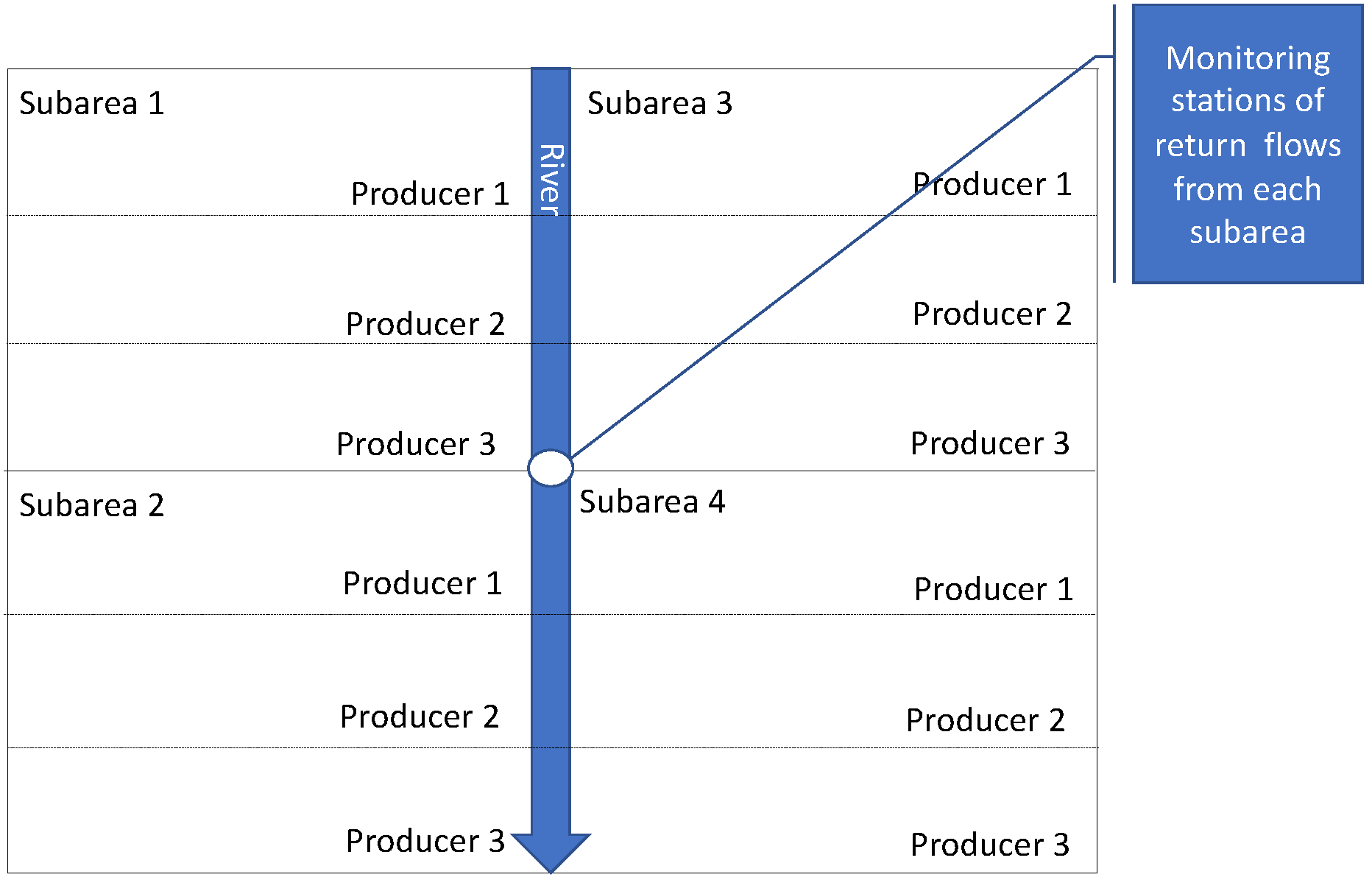
S, that can be used to estimate salt loading. Salt loading is the factor each subarea manager is obligated not to exceed on a monthly and annual basis by the regulator, as defined within the Total Maximum Daily Load (TMDL) allocation for each subarea. TMDLs are the policy vehicles that are used by the US Environmental Protection Agency to limit nonpoint source pollution to levels that do not exceed the assimilative capacity of the receiving water body. TMDLs are keyed into water quality standards or objectives at a compliance monitoring station for the pollutant in the receiving water, and are designed to be protective. The agricultural non-point source pollutant management problem is a typical principal–agent problem under circumstances of asymmetry of information. Hence, we need to introduce several simplifying assumptions. We start by drawing (
Figure 1) a schematic regional setting, using four agriculturally dominated subareas located on the valley floor, and a water body in the form of a river (describing the actual situation in the region that we will empirically analyze). The remaining three subareas are tributary river watersheds where water flow is controlled by upstream dams and reservoirs and whose operation is largely independent of agricultural drainage decision making.
2.2. Real-World Model Fitting
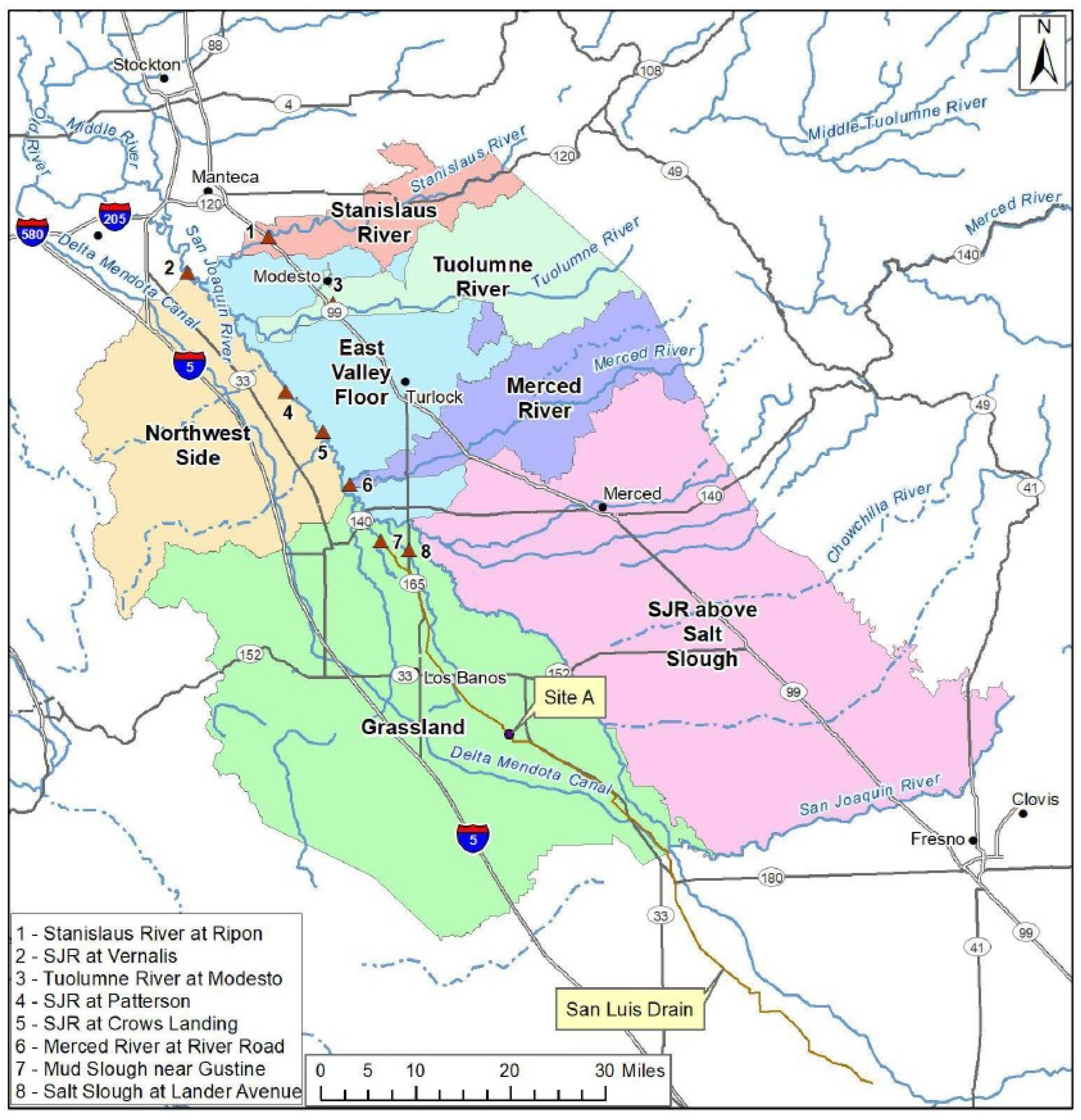
Water supply for the westside of the San Joaquin River Basin (SJRB) is provided by a water agency (e.g., United States Bureau of Reclamation) to the two westside subareas (Grasslands and the North-West Side subareas), according to water contracts negotiated between the water agency and individual water districts within each subarea. The individual water districts, in turn, allocate and distribute water supply according to agreements made with agricultural producers within each subarea. Water supply to subareas on the eastside of the SJRB derives largely from snowpack runoff from the Sierra Nevada Mountain Range, stored in downstream reservoirs along each major San Joaquin River (SJR) tributary. A state government water quality regulator (such as the California State Water Board), with the Regional Water Quality Control Board as enforcer, sets salt load objectives for the Basin in accordance with a Total Maximum Daily Load (TMDL) allocation developed by the Environmental Protection Agency for the basin. The load-based TMDL was further refined to develop subarea-level salt load allocations that take account of different water year hydrology. The conservative nature of the TMDL computation that utilizes the lowest 10% average low-flow condition resulted in allocations that were unattainable without major impact to the agricultural economy in each subarea. Hence, the initial TMDL allocations were replaced by concentration objectives, based on a 30-day running average electrical conductivity (EC), for the most downstream monitoring location on the SJR, Vernalis. A concentration objective allows agricultural producers and other salinity dischargers to utilize more of the available salt load assimilative capacity in the SJR. This initial compliance-monitoring objective has been supplemented with two additional upstream salinity objectives, ostensibly to protect the water quality of agricultural diversions made by westside agricultural producers. These additional salinity objectives are set at 1550 uS/cm year-round, as opposed to the 1000 uS/cm non-irrigation season, and 700 uS/cm objective set at Vernalis. The regulator suggested a number of approaches by which the original salinity load allocations, under the TMDL, might form the basis for salt load reduction strategies or cost allocation in situations where these various salt load objectives were violated.
The salinity load (mass of salt from all producers which is calculated by summing the product of drainage volume and salt concentration from each producer) produced on subarea n is the result of the return flows (drainage) from the agricultural activity of all producers, such that . There is no practical way that the regulator could equitably assign salt pollution levels to the individual agricultural producers or enforce this regulation at a reasonable cost to individual agricultural producers. Therefore, the regulator has chosen to allow stakeholders to internally govern the strategies to attain and abide by river EC objectives, while encouraging stakeholders to consider the subarea as the organizing entity for stakeholder action. Stakeholder compliance is monitored by the Regional Board using data supplied by state and federal water agencies.
To maintain compliance the agricultural producers can dynamically allocate salt loads to each subarea given that available salt load assimilative capacity at each compliance station is the product of the total assimilative capacity (defined by the current flow multiplied by the EC objective) and the current salt load in the river.
The monthly salt load cap can be calculated for each subarea individually based on the calculated TMDL allocations and the current salt loading to the river from each subarea (measured in terms of tons of salt:
SL =
d [salt concentration,
S; volume,
Q]), where
SL is salt load (In the San Joaquin River the current TMDL criterion is a 30-day running average salt concentration that is multiplied by a monthly design flow to determine allowable salt loading). Using this stakeholder-maintained salinity load cap approach subareas would pay a fine (
F) to the regulator, which could be a price per unit of salt load above the cap or some other equitable formula for dividing the fine amongst stakeholders.
F can be specific to each subarea or similar for all subareas (see [
23], for critique on uniform tax).
F is then equitably distributed according to some formula (by land area, drainage volume, incremental salt load etc.) among all
Kn agricultural producers in the different subareas (or by water user associations/districts in each subarea). We assume, for simplicity, that since we have a non-point source salinity management problem where the exact source of salt is not known, the most straight-forward and cost-effective initial approach to distribute
F is to divide it equally per acre of land in production, or per acre–foot of irrigation water supply delivered. These initial approaches ignore the fact that some crops are associated with higher drainage return flow volumes and that subsurface drainage return flow salt loads may be poorly correlated with irrigation applications. Alternative allocation formulas may be relevant and will be considered in the empirical model. We assume that the (hypothetical) subarea manager (While there is no actual subarea manager, it is assumed that the model allocations are respected by the individual farmers and other decision makers at the water district level) has the authority or power to impose these allocations of river salt load assimilative capacity. We also do not want to set an optimal level for
F, but rather take
F as given in the empirical analysis. We will use several levels of
F in a sensitivity analysis to evaluate the effect of
F on the behavior of the agricultural decisionmakers at the subarea level.
An additional consideration is in the temporal administration of fines and fee schedules, which has a bearing on the design of a decision support system to aid the subarea manager to orchestrates stakeholder responses to potential violations of the river salinity objectives. An approach that attempts to respond to potential exceedance of salt load assimilative capacity at each compliance site in real-time would require model simulation tools that ran on a monthly timestep at a minimum. An optimization model would choose between available salt load reduction strategies, purchase of available water supply for dilution purposes, or payment of fines each month. Alternatively, accounting could be postponed until the end of each year and fines imposed retroactively. The latter strategy would rely on uncertainty and the fear of a potential exceedance to motivate compliance. However, the decision tool needed to support this strategy could be simplified to operate on an annual timestep.
2.3. Individual Responses to Water Quality Regulations
We expect that each stakeholder within each subarea will respond to F, depending on the level of F and the conditions (cropping patterns, physical conditions such as soil properties, etc.) in that subarea. In the empirical application, we will look at the effects of surface water and irrigation land and water limits and fees, as these are the main forms of regulation that can affect salinity load in the case of a nonpoint source pollution. In future empirical applications, we propose limits on the output of the model, specifically the salinity loading. Here, we outline the full analytical model.
Given F, each subarea faces the following two options:
- (a)
Maintain the current (status quo) level of salt loading if F the cost of abatement. The cost of abatement could include changing the crop mix and/or land use changes (e.g., fallowing land) (Changes in land use (crop mix or fallowed land) is an important component to maximize revenue and obtain maximum resource use efficiency. In the empirical model, changes in land use is incorporated at a later stage in the model development process), surface and/or subsurface drainage reuse, investing in more efficient irrigation technology, changing irrigation scheduling, and other options.
- (b)
Abate to a level of allowable salt loading than the cap. Each subarea will require abatement activities (detailed below) to the point where the marginal abatement cost equals F.
We consider the abatement in (a) and (b) to be “individual responses” to the salinity management regulation. That is, each subarea acts on its own responses, given its resources and local conditions (In the empirical application section, we also consider some of the individual responses, such as restrictions on water quotas, restrictions on cropping patterns, land fallowing, and investment in water-conserving irrigation technologies, as regulatory-imposed policies).
Each subarea is characterized by an aggregate revenue function (of all agricultural producers within each water district) minus fines on excess salt loading and minus abatement cost, such that
where
is a fine on excess salt loads,
is pollution fine per unit of excess salt load,
is salt load,
is abatement cost, and
is a set of abatement options, such as changing cropping patterns, fallowing land, adopting more efficient irrigation technologies, and investing in monitoring drainage quantity and quality. Each subarea can select one of these abatement options or a subset of the abatement options.
2.4. Allocation of Joint Costs and Benefits in the Case of Individual Responses
In both individual and cooperative responses, we estimate the subarea net benefits as revenues minus variable operational costs and incremental costs. The incremental costs include costs associated with activities that polluters introduce to the agricultural production process in response to the regulatory objectives or constraints on input use imposed by the regulator for each subarea. In the case of a fine imposed on the entire region for exceeding the pollution EC objective, the subarea level of fine is allocated, based on several allocation principles, and the subarea amount of fine, , is added to the incremental costs. In the case of cooperation among the subareas; we estimate first the regional net benefits to the entire region. The value of the regional benefits is obtained by running a regional optimization model, coined ‘a social planner’ model, which maximizes the entire regional welfare rather than looking at welfare of each subarea individually.
Economic theory [
31], suggests that a social planner allocating regional benefits or costs among the agents involved maximizes the joint welfare of the region, subject to physical and institutional constraints relevant to the situation under study. Under a social planner optimization, the region is seen as one unit without political borders. An optimal social planner allocation is considered as first best and serves as reference (benchmark) to which other allocation schemes are compared. Deviations from the social planner outcomes represent inefficiency (welfare loss) of the alternative allocations.
Once a regional social planner allocation solution has been found, the regional gains (either welfare benefits or savings of joint costs—such as regulatory fines) must be distributed among the regional parties. We will consider a couple of schemes for the allocation of the joint benefits or the costs of pollution control, or regulatory fines, among resource management regions, namely, the subareas (and the individual farmers in each subarea). For example, allocation of benefits or fines could be based on annual drainage flows or based on irrigated area. The likelihood of subareas forming stable coalitions aimed to reduce salt loads can be measured by comparing the empirical attributes of the standard allocation schemes with game theoretic allocation schemes whose acceptability and stability can be measured. We introduced several allocation schemes, based on the subarea’s contribution of pollution load and consistent with the strategy described previously [
32].
2.4.1. Allocation of Regulatory Fines Based on Surface Water Applied
This allocation scheme simply suggests that each polluter (subarea) will be charged in proportion to the volume of surface water applied on that subarea. Therefore, the cost to subarea
j is
where
is the regulatory fine allocated to subarea
j;
F is total regional regulatory fine. This scheme allocates all the regulatory fine among all
N subareas.
is the volume of surface water applied for irrigation in subarea
j (a summation over all irrigated area). The disadvantage of this regulatory method is that it does not target those stakeholders who physically discharge to the SJR and not take into account the significant reuse that occurs in some areas that helps to curtail salt loading to the river. It is a blunt policy instrument that is nonetheless relatively easy to administer.
2.4.2. Allocation of Regulatory Fines Based on Total Irrigation Water Applied
This allocation scheme simply suggests that each polluter (subarea) will be charged in proportion to the total volume of water applied (surface water + groundwater + recycled wastewater) on that subarea. Therefore, the cost to subarea
j is
The drawbacks to this policy are the same as those of the prior policy, although, it does account for groundwater use that can add significant salt to the total salt discharged from each region, since the EC of groundwater is typically more than double that of applied surface water on the westside of the Valley, and more than four times the average EC of eastside water applications.
2.4.3. Allocation of Regulatory Fines Based on Salt Load Generation
The allocation scheme in (11) simply suggests that each polluter (subarea) will be charged in proportion to the amount of salt load it generates. Therefore, the cost to subarea
j is
where
is the quantity of salt load generated by subarea
j.
This policy is the most equitable but also the most difficult to administer since current monitoring and modeling is insufficient to accurately measure or estimate the salt load export from each subarea. Current models are not capable of recognizing the amount off drainage reuse within each subarea.
2.4.4. Allocation of Regulatory Fines Based on Cultivated Area
The allocation based on cultivated area is built on a similar rule as in Equation (12), except that
is cultivated land and not disposed drainage.
where
is the cultivated land area in subregion
j.


