Neural Structures to Predict River Stages in Heavily Urbanized Catchments

Abstract

Accurate flow forecasting may support responsible institutions in managing river systems and limiting damages due to high water levels. Machine-learning models are known to describe many nonlinear hydrological phenomena, but up to now, they have mainly provided a single future value with a fixed information structure. This study trains and tests multi-step deep neural networks with different inputs to forecast the water stage of two sub-alpine urbanized catchments. They prove effective for one hour ahead flood stage values and occurrences. Convolutional neural networks (CNNs) perform better when only past information on the water stage is used. Long short-term memory nets (LSTMs) are more suited to exploit the data coming from the rain gauges. Predicting a set of water stages over the following hour rather than just a single future value may help concerned agencies take the most urgent actions. The paper also shows that the architecture developed for one catchment can be adapted to similar ones maintaining high accuracy.

1. Introduction

Forecasting flows of rivers in heavily urbanized catchments is challenging because of the high runoff caused by impervious surfaces and the relative potential risk for the local population. The European Environment Agency attributes one-third of the damages caused by natural disasters to floods. Since 2000, floods in Europe have caused at least 700 deaths and at least EUR 25 billion in economic losses. Between 1998 and 2005, northwestern Romania, southeastern France, central and southern Germany, northern Italy, and eastern England experienced the highest concentration of repeated flooding. The situation has been similar in Switzerland [1]. The coming decades will likely see more frequent flood occurrences in Europe and, consequently, more significant economic damages due to the combined effects of climate change and expanding urbanization [2,3,4]. In addition, land-use changes, namely the reduction of permeable soil, will further increase the peak discharges of floods by modifying the rainfall and snow-melt infiltration and runoff on the land surface into streams.

Together with risk-based spatial planning and the construction of defense works, one of the key tools to mitigate high flow detrimental effects is the availability of adequate warning systems that can provide the agencies in charge with sufficient time for an intervention. The efficacy of such Early Warning Systems is strictly related to the lead time of the forecast before a critical event occurs. Unfortunately, the heavily urbanized conditions of many regions in the world have increased the volume and speed of floods, decreasing the effectiveness of traditional hydrological forecasting models [5]. This paper tackles these problems by exploring different neural network architectures to predict the flows of two urbanized catchments on the Italian-Swiss side of the Alps: the Lura and Laveggio rivers. They represent interesting case studies due to their fast runoff and the damages that their floods cause.

A flood event is defined by extremely large values of irregular and rare flow occurrences [6]. In particular, this study interprets flooding events as a significant variation of the river’s stage within a short time, rather than events with long return times. The developed neural predictors differ in the internal structure of their component nodes and in terms of information used to issue the forecast.

Machine learning (ML) methods, and neural networks in particular, have already been effectively adopted to forecast hydrological phenomena characterized by complex and strongly nonlinear relationships, such as those occurring in urbanized catchments. Using traditional feed-forward (FF) neural architectures, such applications date back to the end of the past century. For instance, Campolo et al. [7] predicted the Tagliamento River flood events in the northeast of Italy one hour ahead. The authors considered the information provided by a hydrometer and several rain gauges without integrating the rainfall over the basin, as is standard in water balance studies. The same authors in [8] forecasted floods of the Arno River in Tuscany, Central Italy, proving the relevance of autoregressive components (i.e., the river antecedent stages) in water level predictions. Tayfur et al. [9] developed a neural network model for the upper part of the Tiber River basin, again in central Italy, to predict flood peaks. The authors conclude that artificial neural networks outperformed the modified Muskingum and the numerical solutions of the St. Venant equations in forecasting individual storm hydrographs. New dynamic network architectures far exceed physical and conceptual models during critical episodes when the computational time of these numerical models can be a limiting factor and not in line with real-time forecasting purposes [10]. Abbot and Marohasy [11] compared several physical-based and ML predictors in Queensland, Australia, and proved the superior accuracy of the ML models. Liu et al. [12] utilized long short-term memory (LSTM) neural networks to simulate rainfall-runoff relationships for catchments with different climate zones in China. These results are compared to the conceptually based Xinanjiang rainfall-runoff (XAJ) model; authors assessed comparable quality predictions between models, concluding that LSTM represents an efficient hydrologic modeling approach. Apaydin et al. [13] performed a comparative analysis of several recursive neural network (RNN) architectures (Bi-LSTM, LSTM, RNN, GRU) for reservoir inflow forecasting in Turkey. LSTM nets succeeded in simulating peak flow periods accurately. The results in [14] underline the LSTM structure’s potential for rainfall-runoff and large-scale regional modelling using catchment attributes and meteorology for large-sample studies in 241 basins in the USA. Hu et al. [15] proved that LSTMs lead to better performance compared to FF neural networks due to their ability to learn long-term dependencies representing, for instance, storage effects within catchments, which may play an essential role in hydrological processes. Kabir et al. [16] compared convolutional neural network (CNN) predictions with the outputs produced by a 2D hydraulic model (LISFLOOD-FP) in Carlisle, UK: the CNN model is highly accurate in capturing flooded cells, as indicated by several quantitative assessment metrics. CNNs are a class of deep neural networks, most commonly applied for image analysis. However, they have shown high accuracy in correspondence of 1D time series data, such as those used for speech recognition [17] and text classification [18]. Ragab et al. [19] showed that the accuracy of CNNs increased faster than other neural prediction approaches, such as LSTM, due to their low computational requirements in real-time and low-cost implementations; however, other recent studies (e.g., [20,21,22]) concluded that LSTM represented the most advisable choice.

The last years have witnessed a steady growth in the application of neural predictors to river flow forecasting, as shown, for instance, by the review papers of Mosavi et al. [23], Tayfur et al. [24], Zounemat-Kermani et al. [25], or Ghorpade et al. [26]. Indeed, Google Scholar quotes over 37,000 articles concerning the use of neural networks in river flow forecasting in 2020–2021, with an increase of about 18% compared with the preceding two years.

Besides the internal structure, another essential aspect in the definition of the predictor model is the type and amount of information used to compute the forecast. For example, the number of preceding autoregressive river flows can be set by trial-and-error, but the number of rain gauges, their possible integration, or other input variables may also be considered. For instance, in ref. [27] and, more recently, in ref. [28], the preceding rainfall or the basin saturation state are used as input to the neural predictors. Refs. [29,30] use measured or forecast precipitation, while refs. [31,32] use radar observations and derived products, and ref. [33] integrates them with satellite sensor data.

Although the state-of-the-art suggests investment into neural networks implementation in hydrological applications, unexplored aspects and improvement margins are still evident in the works analysed above; this study explores and addresses some of these issues. One overlooked aspect central to this study concerns how the neural models are trained for forecasting critical episodes, since this is essential to support the decision-making processes. Flood events are the most difficult to predict because of their low frequency of occurrences, and imbalanced datasets can negatively influence many machine-learning algorithms. For that reason, several studies applied undersampling and/or oversampling techniques to increase the frequency of such extreme events (e.g., [34]). Other studies have developed neural networks based on flood events only to manage this issue (see, for instance, [15,35]). Namely, they developed models capable of describing the flood dynamics, but cannot recognize the occurrences of such events in advance. On the contrary, we aim to compare deep neural predictors of water stages and floods without altering the probability distribution of the measured variables. The data used to train the model are not manipulated in any way, maintaining their sequentiality, as well as proportionality, between extreme events and standard situations. Therefore, the approach applied in this study allows the development of models that can be immediately adopted in actual cases. Another peculiar characteristic of the approach adopted is the development of multi-step predictors that provide a sequence of future stage values instead of just a single one for a specific time step ahead. This feature allows for better planning actions during critical episodes.

Different neural network types have been compared in the following analysis, exploiting the same data. More precisely, each neural network implementation has been differentiated into autoregressive and multivariable models that use different input information. In this way, the analysis will quantify the added value carried by the additional information at different frequencies and trade it off with the performance improvements. Furthermore, to better appreciate the performance of the proposed neural network structures, we compare their performance with two classical benchmarks: a persistent predictor (i.e., the current water stage value is used to predict the future one) and standard FF architecture. Finally, the paper explores the possibility of transposing the neural network architecture optimized for the Lura River to forecast the stages of another catchment in the same area with similar characteristics, the Laveggio River.

The results of the set of neural models presented in the following sections may help environmental authorities to better trade-off the model complexity and information requirements with the accuracy of forecasted values, and thus select the implementation that better suits their practical needs.

The paper is organized as follows. The next section describes the study areas and the related data used in the analysis. The following section presents the tools and methodology used, the models’ architectures, and the evaluation metrics considered. The fourth section shows the results obtained using the different models, while the last draws some conclusions about possible future uses of the developed models.

2. Materials and Methods

2.1. Case Studies Description

The case studies considered, the Lura and the Laveggio rivers, are represented in Figure 1 in their subalpine territorial context. Each domain is detailed in the following.

2.2. The Lura River Basin

The Lura stream originates at 450 m above sea level from the lower area of a hilly region across the Swiss-Italian border. It flows north–south for about 45 km, and its catchment covers 130 km² at the junction with the Olona River.

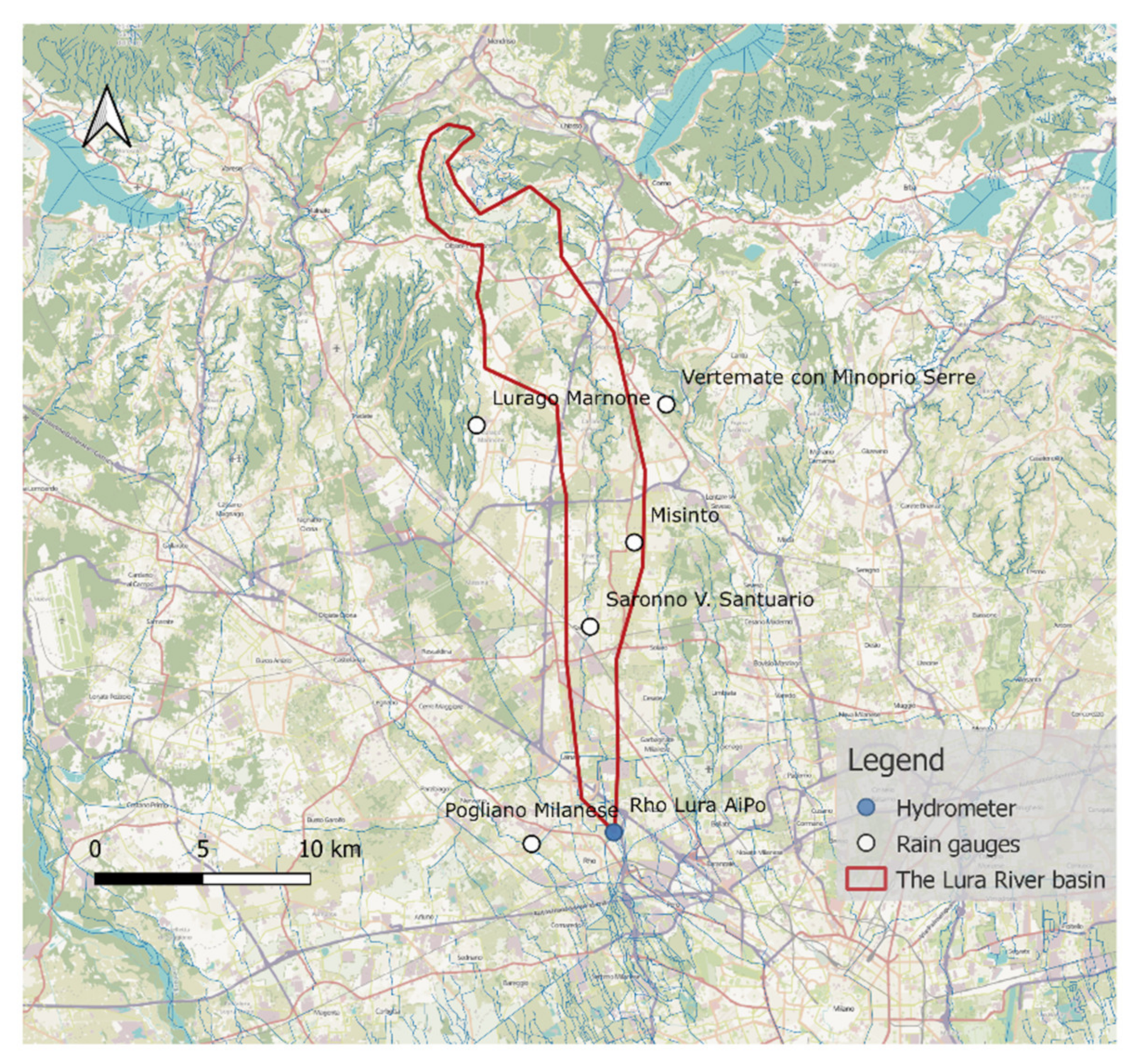
The catchment, represented in Figure 2, is characterized by intense and steadily increasing urbanisation in the southern part [36], accounting for one-third of the total catchment surface. Consequently, the hydrological response differs according to the area hit by the heaviest precipitation. The basin can be clustered into three main areas: the “natural Lura” consists of the upper part where the catchment has a relevant gradient and marginal urban areas; the “intermediate Lura”, where the river flows through the open flatland occupied by several urban centres; and lastly, the “urban Lura”, in which the stream flows partially covered into an almost totally paved catchment, with limited conveying capacity and absence of expansion areas. Due to these peculiar characteristics, the Lura stream has been affected by several flooding events, mainly originating from the urban stormwater drainage system, which derives its volumes from several inputs [37]. A few decades ago, to mitigate inundation risks at the main urban centres, a diversion channel was created to convey part of the discharge to the CSNO (Canale Scolmatore di Nord Ovest). It constitutes the main hydraulic infrastructure built during the 1980s to reduce floodwater volumes entering the northern Milan metropolitan area. In 2014, some municipalities (Saronno, Caronno Pertusella, Lainate, and Rho) were severely flooded. In the late 2010s, a detention basin of 340,000 m³ was implemented in the “intermediate Lura” to reduce the peak discharge from 70 m³s⁻¹ to less than 20 m³s⁻¹ before entering the urban areas. Despite implementing these structural measures, the lower catchment is still hit by frequent floods due to intense and spatially concentrated storms. As the hydrological concentration time is about 30 min, the current monitoring network detects and transmits the registered data with a 10-min resolution.

2.3. The Laveggio River Basin

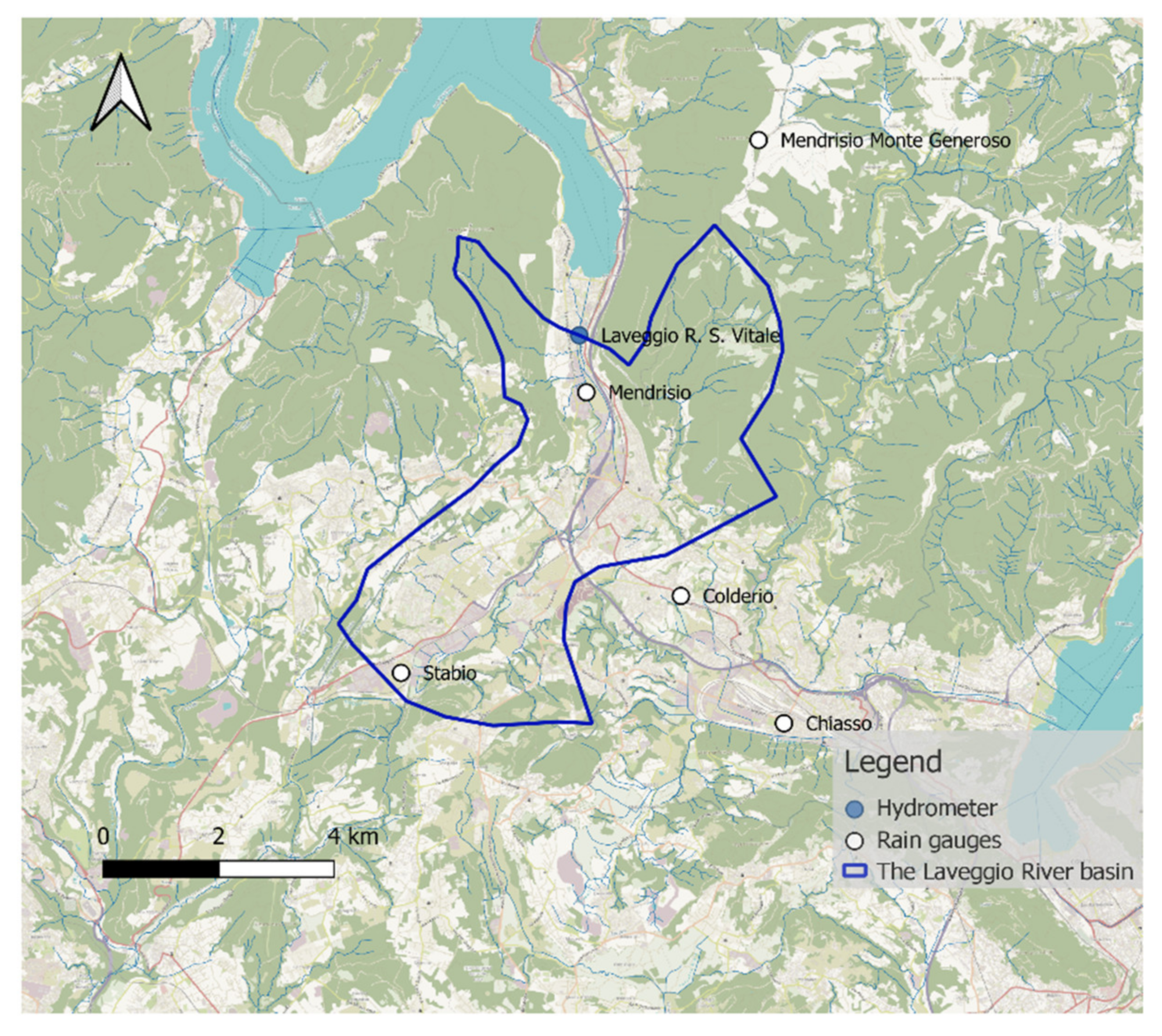
The Laveggio River is a tributary of Lake Lugano, and it flows in the Canton of Ticino, Switzerland, from south to north. It originates near the Italian border and joins the lake in the municipality of Riva San Vitale. The catchment area is about 33 km², as shown in Figure 3.

The Laveggio River is located in three distinct stratigraphic units with different permeability and soil characteristics. The more recent unit (post-glacial) is characterized by prevalent gravel deposits and a strong permeability fed to the east by the limestone karst massif of the Jura age (Morée catchment basin), with a very intense and rapid response to precipitation events. The first river correction works were carried out from 1912 onwards, eliminating the typical meandering course of the river and building embankments, which still feature in the area today. The 1940s were characterized by wide land reclamation works in the area of S. Martino and Prati Maggi (etymologically, Prati Marci). From the 1960s onward, however, the most important change was intense urbanisation, with the development of a large industrial and artisanal zone on much of the flat land around the Laveggio River, exponentially increasing the potential damage and the risk for people and infrastructures. The largest recorded flow event occurred from 13 to 15 September 1995, with a peak discharge of about 70 m³s⁻¹ corresponding roughly to a 30-year return period event. The erosion of the paved riverbed was observed in several areas, with damage to the embankments, but without significant flooding of the surrounding areas. The best-documented events were on 3 May 2002 and 11 November 2014, respectively, with a peak discharge of approximately 58 m³s⁻¹ and 60 m³s⁻¹. The documentation of these two events shows that the channel sections were almost full in both cases. Then, according to the information from the fire brigade, there was only one point where the water overflowed, namely on the left side into the commercial area above Ponte Via Giuseppe Motta. Sandbags have been placed along the channel as a preventive measure during other flooding events since 1992.

2.4. Data Description

In the case of the Lura River, the prediction was based on data collected by a hydrometer operated by Agenzia Interregionale per il Fiume Po (AIPo), together with five rain gauges (Lurago Marinone, Misinto, Vertemate con Minoprio, Pogliano Milanese and Saronno), managed by ARPA—the environmental agency of the Lombardy region. All these measurement stations are represented in Figure 2. Data of the Laveggio River are from the Riva S. Vitale hydrometer, together with five rain gauges (Chiasso, Coldrerio, Mendrisio, Monte Generoso, and Stabio), operated by MeteoSwiss and by the Department of Environment and Spatial Planning of Canton Ticino (OASI database), as represented in Figure 3. In both application domains, data covers from 7 October 2015 to 25 July 2018, with a time-step equal to 10 min, a sufficient frequency to portray the high-speed dynamics of the studied phenomena, i.e., 147,312 records of water stage and precipitation were considered for each domain.

Available records were divided into three subsets respecting the temporal order of observations: training, validation, and test sets, respectively, composed of 70%, 20%, and 10% of available data. The training set was used to identify model parameters, while the validation set served to find the model architecture: training and validation data constitute the calibration data on which models are based. The test set was employed to assess model performance on previously unused data. For the Lura River, it was composed of 2454 hourly sequences of water stage records, 65 of which exceeded the flooding threshold, i.e., 2.67% of the total. For the Laveggio River, the test set comprised 2427 hourly sequences, where 28, i.e., 1.15%, were above the flood threshold (detailed later).

Data were comprised of attributes with varying scales, i.e., water stages and rainfall records, so they were normalized to the interval 0 to 1. This procedure benefits many machine learning algorithms, such as neural network training.

The forecasting task was approached as a regression problem to develop autoregressive and multivariable models. Autoregressive models comprise a single series of water stages. On the other hand, multivariable models include more than one observation for each time step, i.e., water stage observations complemented by rain gauge records.

Neural networks can be trained in different ways: in this study, the supervised learning method was implemented where model outputs are compared to actual values. In particular, river water stages $\widehat{y}$ were predicted up to h time steps ahead by exploiting the information available at time t, when the forecast was issued. Such information constitutes the model input and always includes d samples of the actual water stage (y), as shown by Equation (1). The implemented models f_a thus work as multi-output—the forecast is the future sequence of values along the prediction horizon h:

$$\left[\widehat{y}\left(t+h\right),\dots ,\widehat{y}\left(t+1\right)\right]=f_a\left(y\left(t\right),y\left(t-1\right),\dots ,y\left(t-d+1\right)\right)$$

(1)

The multi-output approach can better support the decisions of the concerned agencies by avoiding the standard recursive method. Most studies develop a single-step ahead predictor, whose output is reused to forecast the following steps: this approach may result in limited performance [35,38]. On the other hand, developing models for multi-step forecasting means that the functions mapping current information to the future water stages are optimized over the entire forecasting horizon h [39]. This parameter will be assumed to be equal to six to obtain at each time step a vector of outputs covering the evolution of the water levels in the next hour. Indeed, an hourly prediction horizon can help issue flood warnings and undertake the most urgent mitigation actions. Then, it could be complemented by more extended horizon forecasts in the future when precise rainfall predictions will be available.

This study develops predictive models for forecasting future water stages under two different frequencies of information update: 60 min, i.e., the forecast is issued every hour for the following six ten-minute intervals, or 10 min, for the same intervals ahead. In this last case, there will be more than one forecast for the same clock time, and they will possibly become increasingly accurate as that time approaches. This may be useful to follow the most critical episodes’ evolution closely. The input–output patterns implied in the supervised learning are thus defined differently for the input update frequency of 60 min and 10 min, as shown in

Table 1. Example of the input–output patterns (time step equal to 10 min) for models with an input update frequency of 60 (a) and 10 min (b). In the autoregressive approach, the input vector v only contains previous water stages y; in the multivariable approach, the rainfall records are also included.

(a)

Input

Output

t = 6

v01

v02

v03

v04

v05

v06

$\widehat{y}$07

$\widehat{y}$08

$\widehat{y}$09

$\widehat{y}$10

$\widehat{y}$11

$\widehat{y}$12

t = 12

v07

v08

v09

v10

v11

v12

$\widehat{y}$13

$\widehat{y}$14

$\widehat{y}$15

$\widehat{y}$16

$\widehat{y}$17

$\widehat{y}$18

…

…

(b)

Input

Output

t = 6

v01

v02

v03

v04

v05

v06

$\widehat{y}$07

$\widehat{y}$08

$\widehat{y}$09

$\widehat{y}$10

$\widehat{y}$11

$\widehat{y}$12

t = 7

v02

v03

v04

v05

v06

v07

$\widehat{y}$08

$\widehat{y}$09

$\widehat{y}$10

$\widehat{y}$11

$\widehat{y}$12

$\widehat{y}$13

…

…

. It is interesting to note that, in Table 1b, data are moving along just a one-time step, while the prediction still concerns the following six water level values.

2.5. Multivariable Models: Rain Gauges and Total Rain Scenarios

In the case of the multivariable modelling approach, two different input scenarios were considered: the total rain scenario and the rain gauges scenario. In the total rain scenario, models f_t are fed by an estimate r(t) of the total precipitation over the catchment, computed from all the gauge measurements together, i.e.,

$$\left[\widehat{y}\left(t+h\right),\dots ,\widehat{y}\left(t+1\right)\right]=f_t\left(y\left(t\right),y\left(t-1\right),\dots ,y\left(t-d+1\right), r\left(t\right),r\left(t-1\right),\dots ,r(t-d+1\right))$$

(2)

Finally, the rain gauges scenario includes the time series of each rain gauge r_i(t), contributing individually as model input, as in Equation (3).

$$\left[\widehat{y}\left(t+h\right),\dots ,\widehat{y}\left(t+1\right)\right]=f_r\left(\begin{array}{c}y\left(t\right),y\left(t-1\right),\dots ,y\left(t-d+1\right),r_1\left(t\right),\dots ,\\ r_1\left(t-d_1+1\right),\dots ,r_n\left(t\right),\dots ,r_n\left(t-d_n+1\right)\end{array}\right)$$

(3)

As is already well known, an estimate of the total rain can be obtained by many different approaches (e.g., Kriging, Splines, …). The classical Thiessen method has been applied here, not implying any computational overload. The Thiessen or Voronoi polygons developed by Thiessen [40] assume that measured amounts of precipitation at any station can be applied halfway to the next station in any direction, which means that rainfall, at any point, is equal to the observed rainfall at the closest gauge. The choice of using the Thiessen method instead of a more sophisticated one is supported by the attempt to determine the degradation of the forecast performance in the worst case. Evidently, with a more accurate interpolation, intermediate results can be obtained between those of the individual gauges and the polygon interpolation.

Furthermore, the use of an aggregation method allows consideration of cases where, for any reason, one or more rain measures are missing, which is likely to happen in real applications. Adopting this approach, the forecast can be issued even if just one gauge is active. On the contrary, this would not be possible using the rain gauge scenario.

2.6. Neural Networks

This study explores two different structures that seem particularly suited for the flood prediction task: CNN and LSTM, which will be briefly described in the following sections. CNNs are similar static maps, though with a more sophisticated structure, to the traditional FFs, while LSTMs belong to the class of recurrent neural networks (RNN), namely nets able to solve the forecasting problem from a dynamic perspective. Indeed, RNNs involve modification of the original feed-forward structure, allowing for feedbacks between layers and the existence of a neuron’s internal state that stores information over time.

2.6.1. Convolutional Neural Network

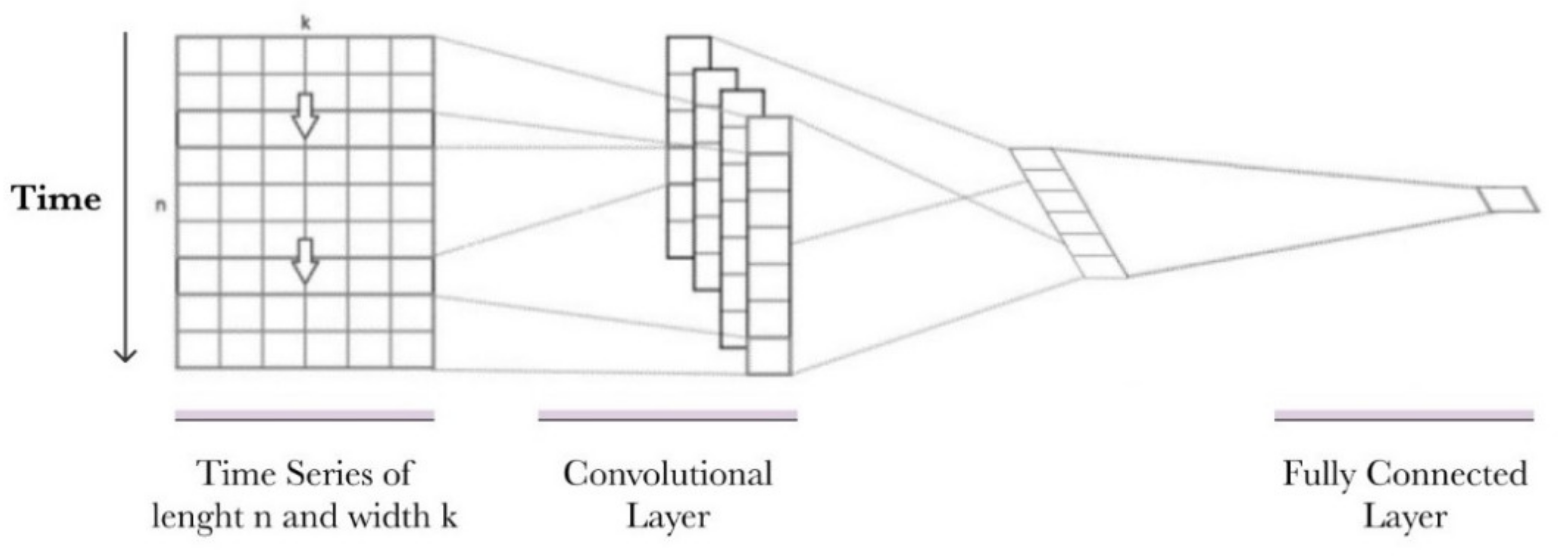
A CNN is made up of several components similar to our visual cortex. They have deep learning (DP) architecture, initially developed for 2D image data. However, they have recently been used also for 1D data, such as sequences of texts and time series. CNN nets can learn how to automatically extract, from the raw data, relevant features that are useful for the problem being addressed when the data have strong spatial and/or temporal correlations. Operating on 1D data, CNNs read across the sequence of lagged observations, detecting the most salient elements for the prediction. The implementation of an autoregressive model results in a 1D-CNN. In the case of a multivariable model, a CNN model made by two 1D-CNN layers for each input series is implied; the prediction is obtained by subsequently combining their outputs.

Figure 4 shows that a CNN net is mainly composed by:

• The convolutional layer. It plays a crucial role in CNNs. Convolution is a linear operation extracting features from inputs through a small moving filter called the kernel. An element-wise product between each kernel element and the input is calculated, obtaining a feature map. The two key hyperparameters that define the convolution operation are the size and number of kernels. Multiple kernels are considered, so this procedure is repeated multiple times, returning different feature maps. The outputs of this linear operation are then passed through a nonlinear activation function, such as a rectified linear unit (ReLU);
• The output feature maps. The previous outputs are transformed into a 1D vector and connected to one or more dense or fully connected (FC) layers in which every input is connected to every output. This last layer maps the extracted features into the final output.

2.6.2. Long Short-Term Memory Neural Network

LSTMs [41] are among the most used RNNs in time series analysis due to their ability to detect and store temporal and spatial dependencies between data. The LSTM shows excellent potential in modelling the dynamics of natural systems, as already noted in the Introduction. The applications of LSTM networks range over several fields, including geology [42], energy [43], air quality modelling [44], economy [45], and meteorology [46]. LSTM neural networks can store information about past data, avoiding excessively increasing the dimension of the network itself.

Like all RNNs, LSTMs also have the form of a chain of cells, each with the interconnected structure shown in Figure 5. In addition to the output, the cell updates a state value that runs straight down the entire chain and is the core of the LSTM inner structure. An LSTM cell has three gates that modify the cell state by removing and adding information:

• The forget gate decides what information shall be filtered from the cell state by looking at the previous hidden state h(t − 1) and the current input x(t);
• The input gate is responsible for updating the cell state c(t). In the input gate, sigmoid and tanh functions combine the previous hidden state h(t − 1) and the current input x(t). The cell state is affected by both forget and input gates (c(t));
• The output gate defines the following hidden state h(t) based on the previous hidden state h(t − 1), current input x(t), and the newly modified cell state c(t). The hidden state h(t) and the new cell state c(t) move forward in the neural chain.

Through these gates, the LSTM cells modulate the effect on the output of the internal memory, which stores the information gathered from past inputs.

2.7. Model Architecture

The implementation of neural networks requires the determination of hyperparameters, which cannot be estimated from data, such as the number of hidden layers and neurons, the input variables lag (d), the activation function, the training algorithm, as well as the performance metric to be optimized. Some guidance on choosing the hyperparameters’ values can be found in the literature, but, basically, the determination of a neural network architecture remains a trial-and-error process, where some values must necessarily be fixed a priori to avoid an overwhelming complexity.

Indeed, we fixed the number of LSTM internal layers to one to provide a fair comparison among models,

Table 2. Hyperparameters of LSTMs in autoregressive and multivariable approaches.

LSTM Hyperparameters	Autoregressive Model	Multivariable Model
Batch-size	64	32
Learning rate	0.001	0.001
Epochs	15	30
Activation function	relu	relu
N. hidden neurons	10	20

, while for CNN nets, the number of layers was the same as the time series involved as inputs, indicated as ‘n.features’ in

Table 3. Hyperparameters of CNNs in autoregressive and multivariable approaches.

CNN Hyperparameters	Autoregressive Model	Multivariable Model
Batch-size	32	16
Learning rate	0.001	0.001
Epochs	20	25
Activation function	relu	relu
Convolutional layers	1	2 × n.features
Kernel size	3	3
Filters	64	32
Fully connected layers	1	2

. In addition, the delay parameter d was set equal to six based on experiments. Indeed, this value leads to the most accurate estimates for all the models, closely following the natural dynamic of the local hydrological phenomena. Finally, all other hyperparameters have been tuned by a grid-search optimization, namely evaluating a model for every combination of possible values within a discrete set.

Table 2 and Table 3, respectively, show the resulting architectures for LSTM and CNN neural models. The hyperparameters obtained from this extensive search on the Lura River have been subsequently applied to the Laveggio River.

All models developed in this study are trained using the efficient Adam version of the stochastic gradient descent. The loss function is represented by the mean squared error (MSE) average value over the entire forecasting horizon h (Equation (4)). Indeed, the MSE is the most commonly used metric in regression models:

$$\mathrm{MSE}=\frac{1}{N}{\displaystyle \sum }_{i=1}^N{\left(y_i-{\widehat{y}}_i\right)}^2$$

(4)

In particular, it indicates the mean square discrepancy between observed data y_i and model predicted value ${\widehat{y}}_i$, with N equal to the cardinality of the training dataset. As is well known, MSE emphasizes the contribution provided by more significant errors that correspond to the occurrence of extreme events, in line with the primary objective of the present modelling exercise. Each training takes place twice, randomly varying the weights initialization to avoid being stuck in a particular solution. Models are implemented in Python mainly using the Keras library, with Tensorflow as the back-end.

2.8. Performance Assessment Metrics

Since the problem is framed as a regression problem, three additional metrics have been computed: RMSE, MAE, and NSE.

The root mean squared error, or RMSE, is defined as the square root of the MSE. Its value is useful since it is expressed in the original units of the target variable.

Equation (5) expresses the mean absolute error or MAE metric that indicates the absolute discrepancy between the observed data y_i and the model estimation ${\widehat{y}}_i$:

$$\mathrm{MAE}=\frac{1}{N}{\displaystyle \sum }_{i=1}^N\left|y_i-{\widehat{y}}_i\right|$$

(5)

Lastly, Equation (6) represents the NSE metric, also known as Nash–Sutcliffe model efficiency, traditionally used to assess the predictive skill of hydrological models [47]:

$$\mathrm{NSE}=1-\frac{{{\displaystyle \sum }}_{i=1}^N{\left(y_i-{\widehat{y}}_i\right)}^2}{{{\displaystyle \sum }}_{i=1}^N{\left(y_i-{\overline{y}}_i\right)}^2}$$

(6)

NSE can range from −∞ to 1. In the ideal case, the NSE should be equal to 1, meaning that the model perfectly interprets the actual data. A model that produces a variance of the estimation error equal to the variance of the observed time series results in a null NSE. In the case of a negative value of the NSE metric, the observed average turns out to be a better predictor than the model. The advantage of looking at NSE is that it is a standardized value, thus allowing comparison of different time series independently on their averages and standard deviations.

One of this study’s aims is to develop models able to predict the occurrence of flooding events in addition to their magnitude. Therefore, to support the decision-making process, results are also interpreted in terms of flood detection. To evaluate the ability of the model to work as a flood classifier, the following ad hoc indicators were introduced:

• I_flood(t) is positive (P) if floods are present in a sequence of values (either real or predicted). Flood sequences are defined as hourly sequences [y(t), y(t + 1),…, y(t + h)] that contain at least one record of water level equal to or greater than a certain threshold (

  Table 4. Thresholds of floods and rapid events in Lura and Laveggio rivers for I_flood and I_rapid indicators.

  River	Flood Threshold (m)	Rapid Increment Threshold (m)
  Lura	1.2	0.20
  Laveggio	0.6	0.08

  ). Conversely, a negative value (N) means there is no flood in the sequence.

  $$\begin{gathered} I_{flood}\left(t\right)=\left\{\begin{array}{c}P if y\ge flood threshold\\ N\hspace{1em}\hspace{1em}\hspace{1em}\hspace{1em}\hspace{1em}otherwise\end{array}\right. \\ \mathrm{with} y \in \left[y\right(t), y(t+1),\dots , y(t+h\left)\right]. \end{gathered}$$

  (7)
• I_rapid(t) indicates whether rapid flow increments occur in a (real or predicted) water stage sequence. Rapid increments are defined as hourly sequences [y(t + h − 1), …, y(t + 1), y(t)] containing at least one value greater than the first of the sequence by the rapid increment threshold (Table 4).

  $$I_{rapid}\left(t\right)=\left\{\begin{array}{c}P if \left[y\left(i\right)-y\left(t\right)\right]\ge rapid increment threshold, \hspace{1em}i\in \left[t+1,t+h\right]\\ N \hspace{1em}\hspace{1em}\hspace{1em}\hspace{1em}\hspace{1em}\hspace{1em}\hspace{1em}otherwise\hfill \end{array}\right.$$

  (8)

These indicators allow evaluation of the classification ability of the models, even if they are not explicitly trained for the classification task. In line with this aim, three additional metrics have been considered: precision (9), recall (10), and their harmonic mean F1 score (11). More precisely,

$$Precision=\frac{TP}{TP+FP}$$

(9)

$$Recall=\frac{TP}{TP+FN}$$

(10)

$$F{1}_{score}=\frac{2 Recall · Precision}{Recall+Precision}$$

(11)

where TP means true positive cases, namely the number of occurrences where the model correctly predicts the positive class (i.e., the actual sequence contains a flood event that the model predicted successfully). On the other hand, TN represents true negative cases (i.e., both reality and prediction include no flood episodes). Finally, FP is false positive, so cases where the model incorrectly predicts the positive class (i.e., the actual sequence is not a flood event, while the model classifies it as such). Consequently, FN represents false negative. Table 4 presents the thresholds used to compute I_flood and I_rapid indicators for both Lura and Laveggio domains. These values are set by referring to the statistical characteristics of water stage time series, as well as historical flooding damages. In general, the water stages of the Laveggio River are lower than those of the Lura River. The thresholds reflect this.

3. Results

CNN and LSTM neural networks have been applied to predict river stages one hour ahead. These models’ predictive power is analysed for both autoregressive and multivariable approaches. The performances are computed on test data employing the evaluation metrics defined in the previous section, and are compared with two standard benchmarks: a persistent predictor that uses the value at time t as the forecast one hour ahead, and a classical FF network.

In the case of the Lura River,

Table 5. The performance of the Lura River’s autoregressive models: average value of the evaluation metrics over the entire test dataset and flood events only.

River	Model	Data	Model	RMSE (cm)	MSE (cm2)	MAE (cm)	NSE
Lura	Autoregressive	All test data	Persistent	11.45	131.17	3.01	0.78
			FF	7.31	53.01	2.04	0.90
			LSTM	7.35	54.11	2.05	0.91
			CNN	7.31	53.43	2.70	0.90
		Extreme events	Persistent	48.63	2393.00	34.23	−0.01
			FF	41.16	1694.01	26.01	0.24
			LSTM	40.51	1641.08	25.91	0.27
			CNN	36.24	1314.02	23.83	0.41

and

Table 6. Performance of multivariable models for the Lura River: average value of evaluation metrics over the forecasting horizon (h) in the entire test dataset and flood events (rain gauges and total rain scenarios).

River	Model	Data	Scenario	RMSE (cm)	MSE (cm2)	MAE (cm)	NSE
Lura	Multivariable	All test data	LSTM—Rain Gauges	6.20	38.53	2.01	0.93
			LSTM—Total Rain	6.02	40.23	2.13	0.93
			CNN—Rain Gauges	6.52	47.08	2.98	0.91
			CNN—Total Rain	6.24	44.20	2.08	0.92
		Extreme events	LSTM—Rain Gauges	29.39	977.64	20.09	0.56
			LSTM—Total Rain	30.35	1042.33	20.90	0.53
			CNN—Rain Gauges	33.45	1262.23	23.36	0.44
			CNN—Total Rain	30.67	1110.57	21.13	0.50

summarise the performance of autoregressive and multivariable models in correspondence to the entire test dataset and flood events only. In particular, Table 5 shows that, over the whole test set, all autoregressive neural networks perform similarly and quite satisfactorily, achieving an NSE equal to 0.90, compared to the 0.78 of the persistent predictor. It is important to underline that flood sequences are just 2.67%, meaning that, in most instances, the prediction is relatively simple. On the other hand, in correspondence to flood events, the persistent predictor scores a negative NSE value, the FF predictor scores 0.24, the LSTM model 0.27, and the CNN model 0.41. 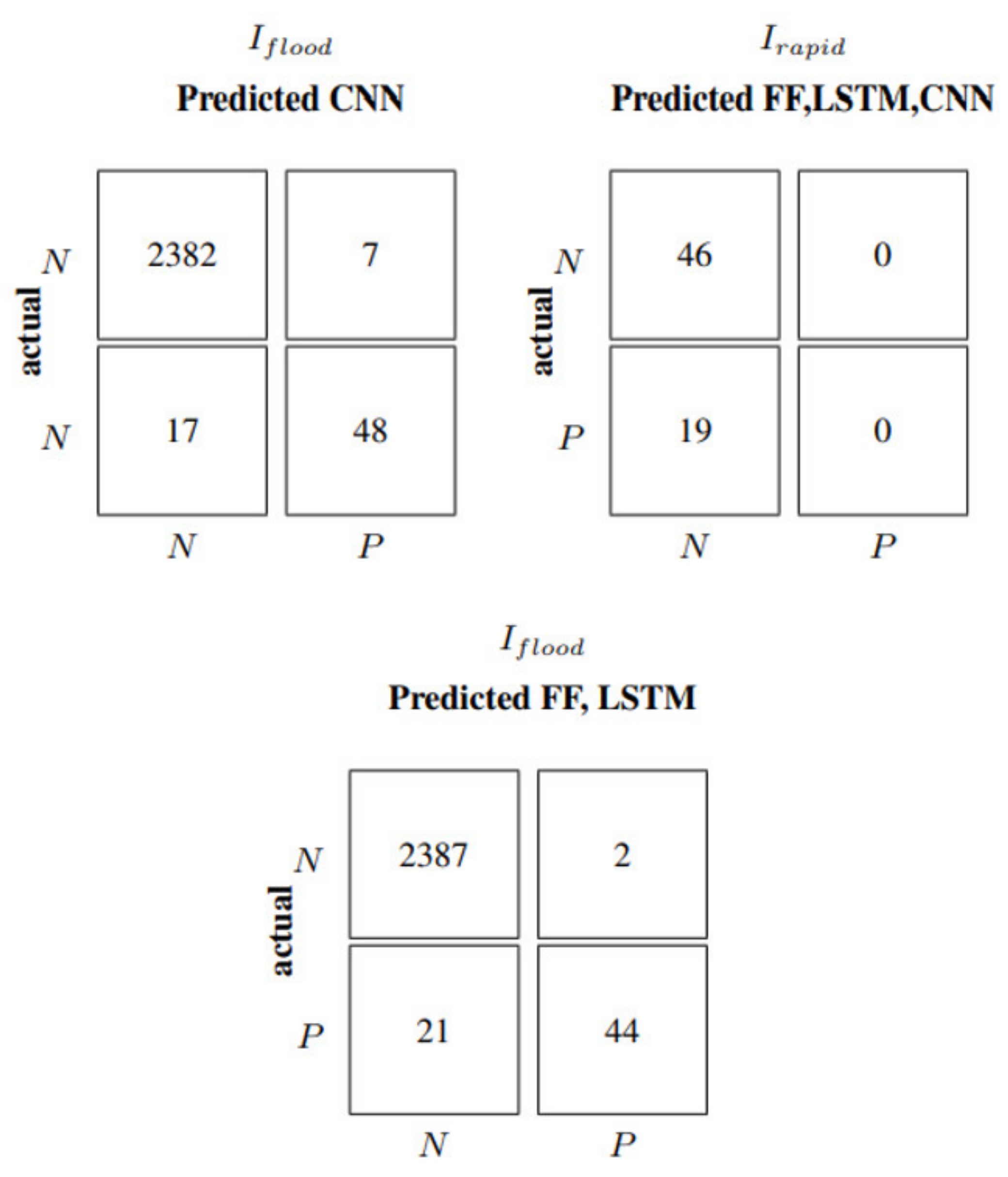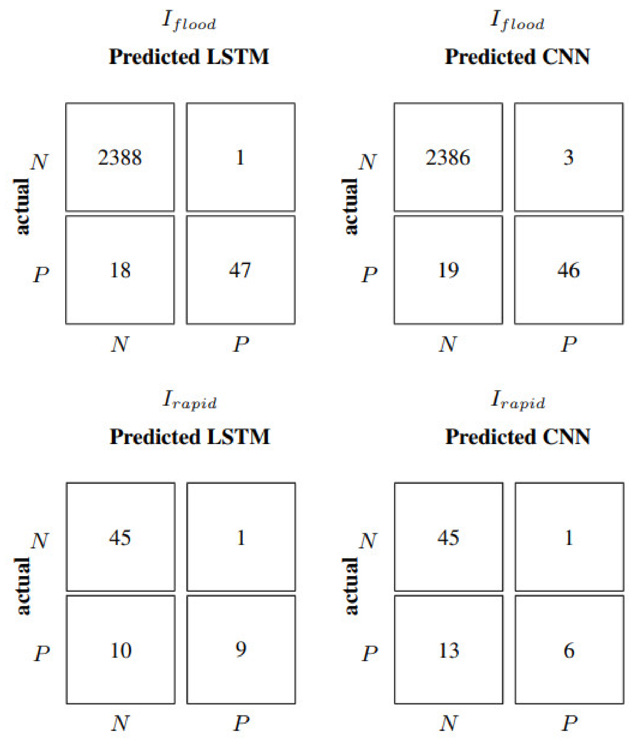The autoregressive FF and LSTM models show similar performances, as is also expressed in Figure 6, where their relative confusion matrices (correct and incorrect number of flood forecasts) coincide.

The performances of the neural predictors are very similar when considering all the test data. In flood conditions (second half of Table 5), CNN provides the best results, followed by LSTM. Despite the improvements compared to the traditional FF networks being limited, we decided to further explore these more modern architectures in the following multivariable approach. It is interesting to note how CNNs perform as autoregressive models: the value of RMSE in flood conditions is 4.27 cm lower compared to LSTMs, and 4.92 cm lower compared to FFs. Flood episodes are defined above 1.2 m, as shown in Table 4; thus, these errors represent less than 4% of the actual values. Results in Figure 6 show that the CNN model performs better than FF and LSTM in terms of correctly predicted floods, even if it also shows a higher value of false alarms or false positives (FP), usually a less severe error than false negatives (FN). This translates into a recall and precision of 0.87 and 0.74 for CNN, while FF and LSTM score 0.95 and 0.68, respectively. The F1 is thus very similar, with 0.79 for FF and LSTM, and 0.80 for CNN. In the case of the persistent predictor, the number of false positives is the same as the number of false negatives; as a consequence, all three classification metrics have an identical value of 0.77. From Figure 6, it is evident that neither model manages to capture rapid events defined by I_rapid. The confusion matrix relative to rapid increments is the same for all neural models with TP equal to zero. Consequently, all the performance indicators related to rapid increments are also null.

The autoregressive term can partly represent the basin saturation state, which influences its base flow. However, the rainfall information could better represent its dynamics. Table 6 shows the performance of the multivariable LSTM and CNN models corresponding to the rain gauges and total rain scenarios in the case of the Lura River. As already discussed, the rain gauges scenario includes the rain gauges taken individually in the model input. On the other hand, the total rain scenario uses an estimate of the total precipitation over the catchment.

Table 6 shows that models perform quite similarly, in correspondence to the entire test dataset, with an improvement of the performance indices between 20% and 30% compared to the autoregressive case (Table 5). Instead, in correspondence of flood events, the LSTM model obtains much better values, with an NSE more than double with respect to the autoregressive case, outperforming the results of the CNN. LSTM also demonstrates the best ability to exploit the information of separate precipitation time series (rain gauges scenario). Table 6 reveals that by predicting floods using rain gauge values, LSTM performs 3% to 6% better than in the total rain scenario.

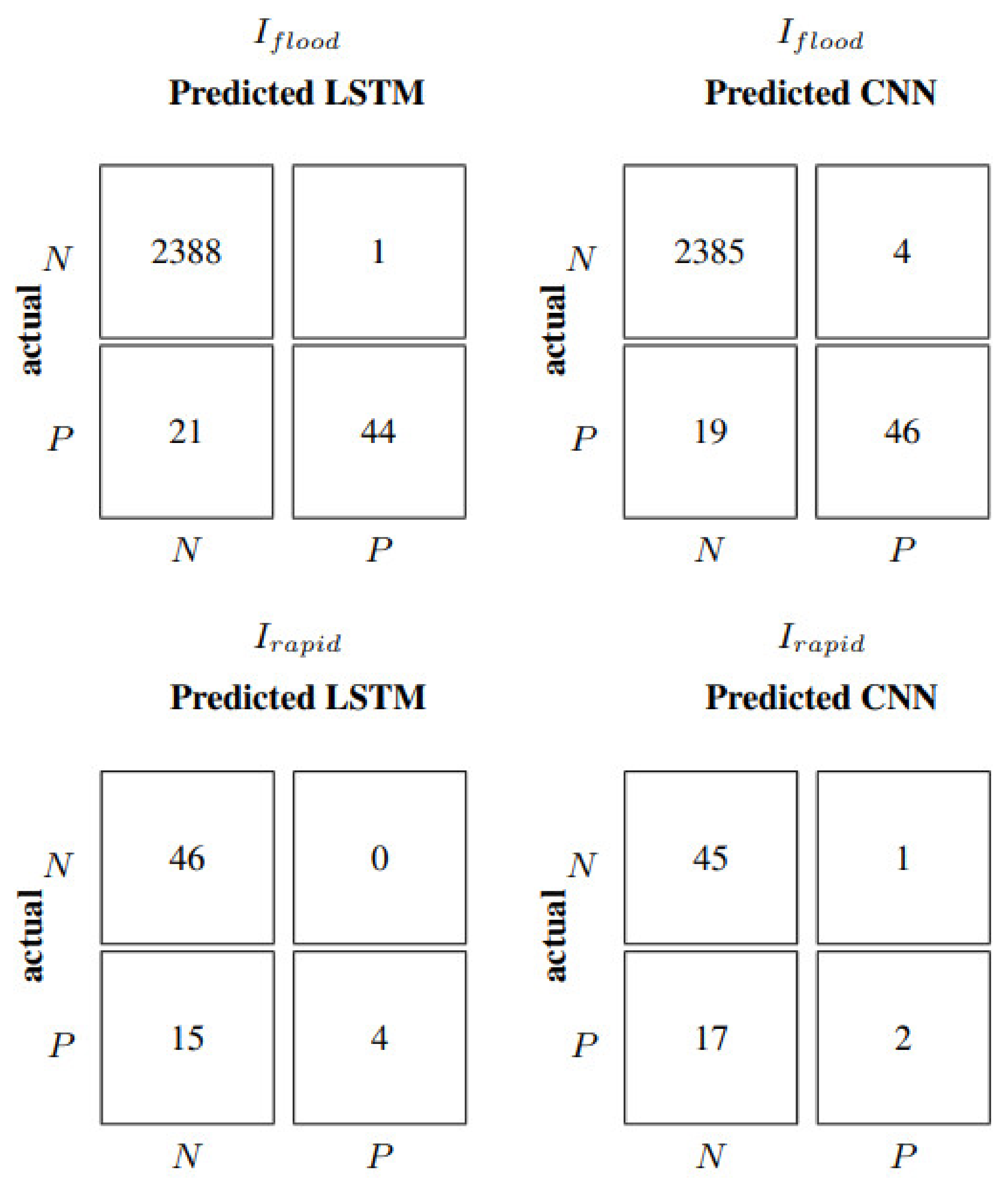
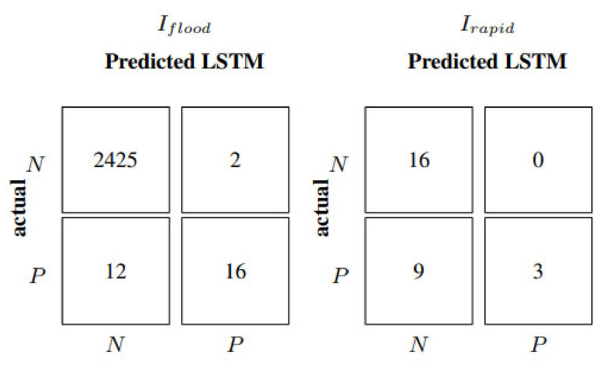
The performance of multivariable models is also expressed in Figure 7 and Figure 8 for the rain gauges and total rain scenarios, respectively. Looking again at the rain gauges case, LSTM and CNN perform similarly in terms of their ability to detect floods, with F1 scores equal to 0.86 and 0.81, precision equal to 0.72 and 0.71, and recall of 0.98 and 0.94, as shown by Figure 7. On the contrary, the LSTM net is demonstrated to be definitely superior in forecasting rapid growth trends, with an F1 equal to 0.62, a precision equal to 0.47, and a recall of 0.90, in comparison to the 0.45, 0.31, and 0.86 of CNN. This is because the CNN does not view data as distributed in time. Instead, they are treated as an input vector over which convolutional read operations can be performed, such as a one-dimensional image. As a result, the CNN model seems effective in predicting future water levels in the autoregressive approach according to its structural property of extracting essential information from 1D data (NSE equal to 0.41, Table 5). However, this net does not reach the same benefit when considering the precipitation records (NSE equal to 0.44 in the rain gauges scenario and 0.50 in the total rain scenario, Table 6). In this case, the LSTM shows more significant potential (NSE equal to 0.56 in the rain gauges and 0.53 in the total rain scenario, Table 6). This is because LSTMs offer native support for sequences, reading one step at a time and building up an internal state representation that can be used as a learned context for making the prediction. For example, in the total rain scenario (Figure 8), the LSTM net predicts flooding events with an F1 equal to 0.80, a precision equal to 0.68, and a recall of 0.97, compared to the 0.80, 0.71, and 0.92 of CNN.

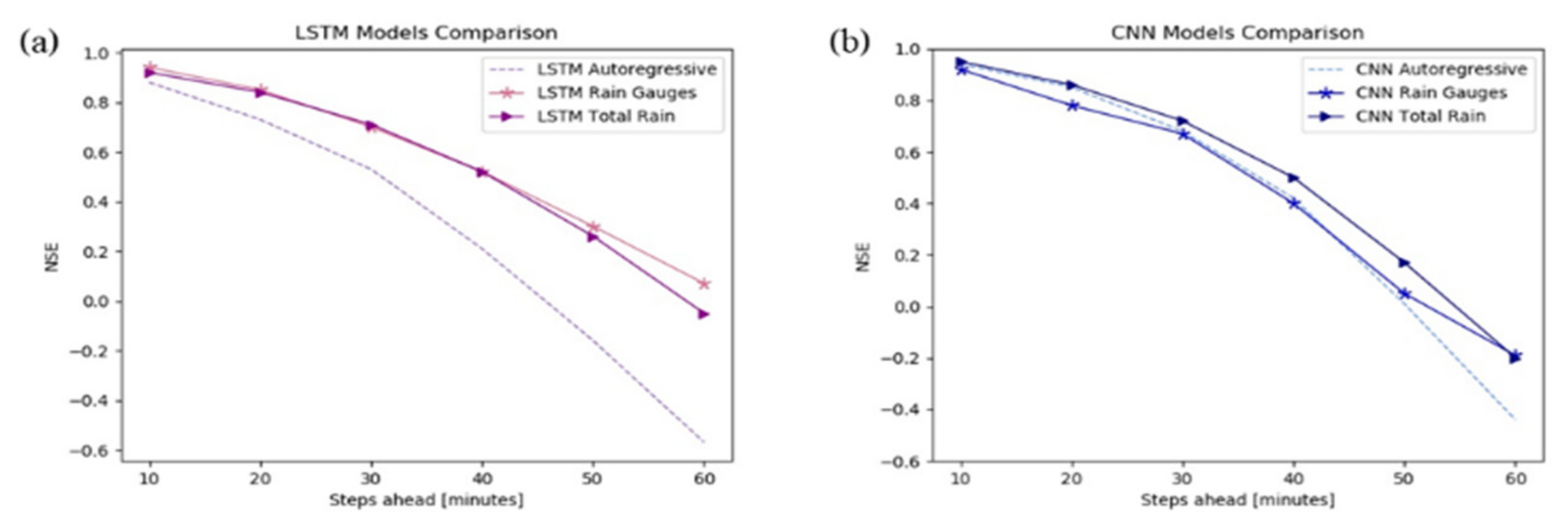
It is common with multi-step forecasting problems to evaluate predictions at different lead times. Figure 9 shows the trend of NSE in correspondence of floods in test data of the Lura River in both autoregressive and multivariable models. The NSE value, as well as the predictive power, regularly decreases over the forecasting horizon. Still, it shows that multivariable models provide better performance with respect to the autoregressive models, particularly in the case of LSTM nets (Figure 9a).

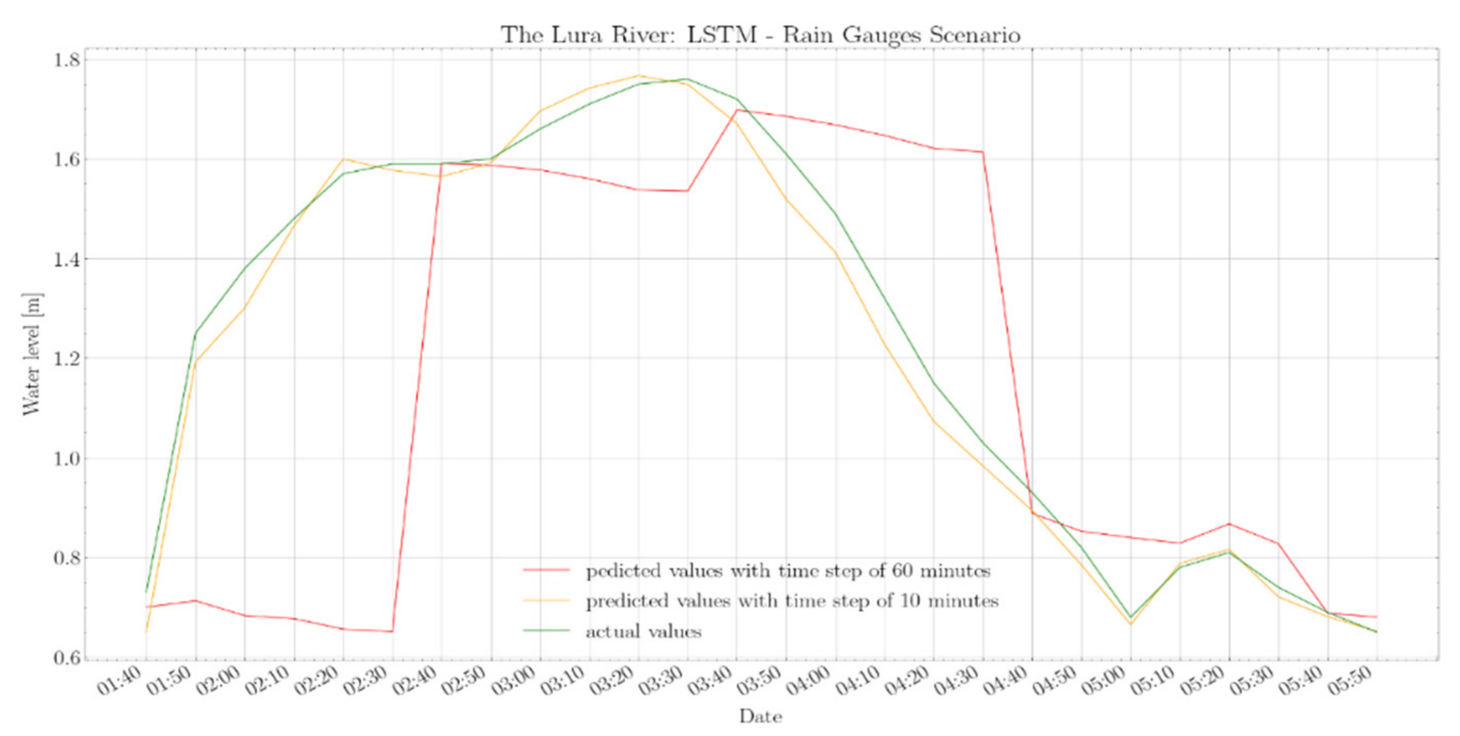
The models presented so far use the previous six observations to get the predictions over the next hour; the forecast is issued every 60 min, and the model input is updated accordingly. In addition, we investigated the performance improvement obtained by providing information more frequently to the model, showing the most accurate predictions, i.e., the LSTM network in the rain gauges scenario.

Table 7. Comparison of multivariable LSTM performance with 60- and 10-min input update frequency for the entire test dataset and flood events only. Rain gauges scenario, Lura River.

		Input Update Frequency
		60 min				10 min
River	Data	RMSE (cm)	MSE (cm2)	MAE (cm)	NSE	RMSE (cm)	MSE (cm2)	MAE (cm)	NSE
Lura	All test data	6.20	38.53	2.01	0.93	3.02	9.32	1.20	0.98
	Extreme events	29.39	977.64	20.09	0.56	9.52	92.16	4.57	0.96

and Figure 9 show the results obtained with an input update frequency equal to 60 min (already shown in Table 6) and 10 min in the case of the Lura River. With an input update frequency of 10 min, the optimized metric is still the average MSE over the next hour, but such a forecast is updated every 10 min, as shown in Table 1b. Therefore, any given water stage is predicted six times with higher and higher accuracy as it approaches.

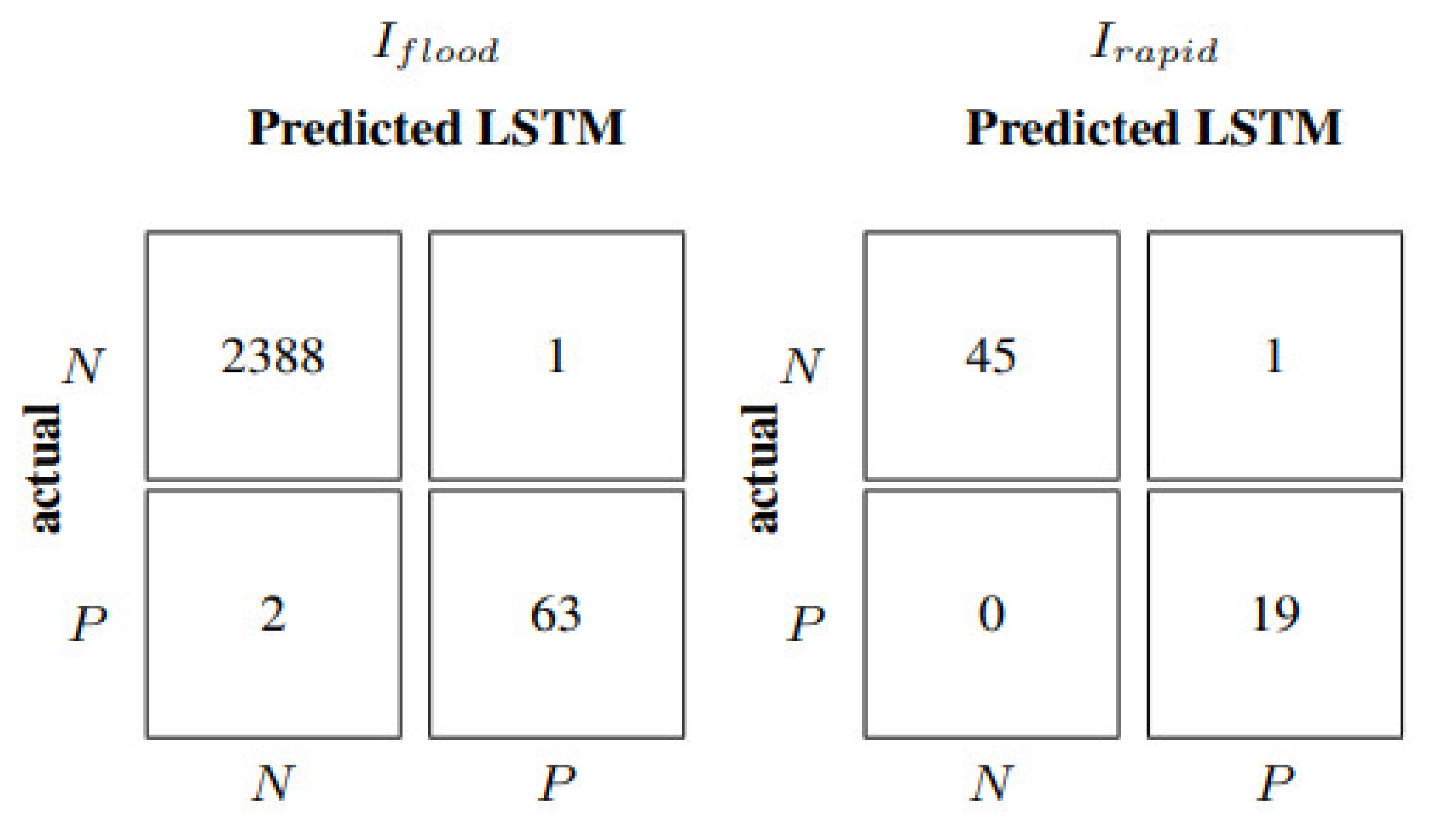
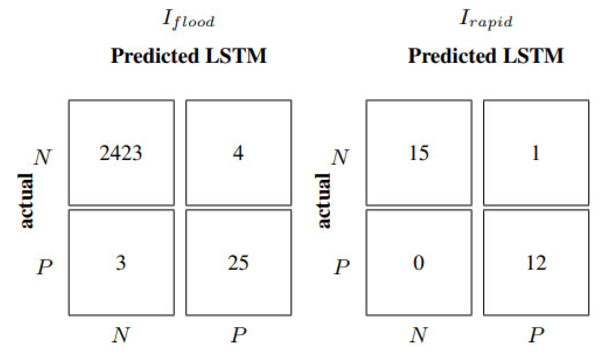
Absolute metrics in Table 7 clearly show how the accuracy is significantly higher in correspondence of flood events when the inputs are updated more frequently. Metrics improve by 40–70% when the entire test dataset is considered. Specifically, in correspondence to flood events, the model with inputs every 10 min leads to a noticeable improvement, ranging from 70% to 90%, also confirmed by a precision value of 0.97, recall equal to 0.98, and an F1 of 0.97 (Figure 10). Therefore, in the case of the rapid growth of water levels, models characterized by an input update frequency of 60 min should be integrated with models with 10-min updates when critical conditions are detected (Figure 11).

Ref. [48] explored the application of support vector machines and artificial neural networks (ANN) on a multivariate set of data, i.e., water basin levels and meteorological data, in the case of the Seveso River. Although the Lura and Seveso Rivers belong to the same hydrological system, the Lambro-Olona basin, using the ANN, the author estimates a value of 0.83 for F1, compared with the 0.97 computed in this study as the flood detection performance for the Lura River. The same is true for another study, conducted on the hydrological basin of the Lambro, Seveso, and Olona Rivers [46], that developed a multivariate DNN to predict water level 30 min ahead.

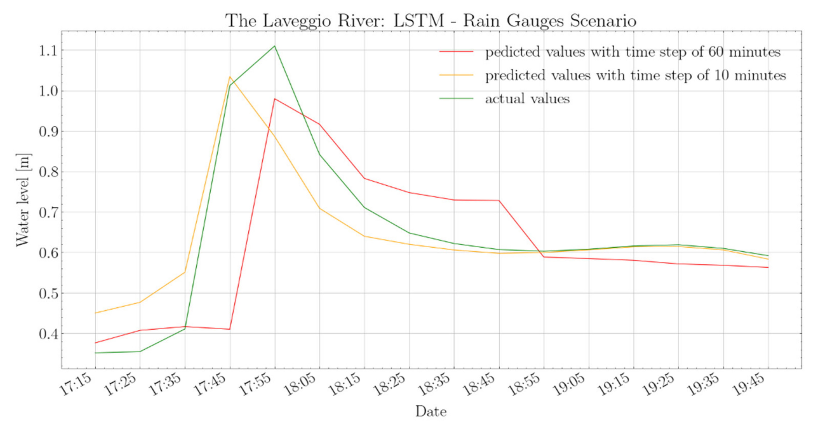
The same architecture of the LSTM neural network in the rain gauges scenario developed for the Lura River has been adopted for the Laveggio River basin after model retraining. Moreover, in this case, both the 60- and 10-min input update frequencies have been applied;

Table 8. Comparison of multivariable LSTM performances with 60- and 10-min input update frequency for the entire test dataset and flood events (Laveggio, rain gauges scenario).

		Input Update Frequency
		60 min				10 min
River	Data	RMSE (cm)	MSE (cm2)	MAE (cm)	NSE	RMSE (cm)	MSE (cm2)	MAE (cm)	NSE
Laveggio	All test data	1.80	3.52	0.61	0.90	0.92	0.86	0.31	0.97
	Extreme events	13.46	200.71	8.80	−0.12	7.70	0.60	4.17	0.63

, and Figure 12 and Figure 13 show the results. In particular, as shown in Table 8, LSTM with input update every 60 min reaches smaller values of the absolute metrics than the Lura case (Table 7), since the Laveggio River has lower water levels. Models’ evaluation metrics in Table 8 allow the estimation of an improvement of about 50–75% over the entire test dataset when updating model inputs every 10 min. In flood events, such an improvement goes from 40% to 99%. Indeed, in correspondence with an input update frequency of 60 min, the LSTM net leads to an NSE equal to −0.12 for flood events, a much less satisfactory performance than in the Lura River case. The negative value of the NSE metric indicates that the model cannot capture the flood dynamics. This can be explained, on the one side, because data used to develop models for the Laveggio River are characterized by very few flood events (as previously discussed), not allowing the neural model to learn the causal relations in critical conditions. Indeed, considering six previous values of water levels and rainfall to predict future water level sequences is suitable when considering the entire test data; however, it becomes insufficient to describe the rare flood dynamics. Conversely, the hyperparameters of the Laveggio River model were kept equal to the Lura River. A specific optimization of the LSTM architecture could have provided better results.

Figure 14 demonstrates how the model better describes the system behaviour with 10 min input frequency, which is also reflected in Table 8 by a 0.63 NSE. Furthermore, the model achieves an F1 equal to 0.96 in the case of rapid events, rather than 0.4 scored by the model with 60-min input frequency (Figure 12 and Figure 13). Therefore, the predictions obtained using a multivariable LSTM with a 10-min input update frequency deliver relevant information and content.

In practice, both the water authorities of Lura and Laveggio use completely different, more physical-based models for their routine forecasting activities. The FEST-WB [49] model is used on the Italian side, and the PREVAH [50] model on the Swiss side. They both require a considerable amount of additional information (air temperature, precipitation, relative humidity or water vapour pressure, global radiation, wind speed, and sunshine duration), as well as a detailed description of the catchment’s physical characteristics. Additionally, they need non-negligible computer power, which is one of the reasons why they are not best suited for forecasting activities in such small catchment areas and with very short response times. For instance, the results of PREVAH on the Laveggio River show a relatively low average NSE, i.e., about 0.53, with this score being computed on calibration data [51]. On the contrary, they may be very useful for planning purposes.

4. Conclusions

This study examined the use of different neural network architectures for river flow forecasting and early warnings of floods. In addition, it deepened some common issues concerning applying such tools, such as training models only on flood events, developing only one-step ahead recursive predictors, handling the probability distribution of the natural phenomena, and exploiting rainfall data.

The results confirmed that deep neural networks have a strong potential to deal with urbanized water catchments and accurately represent the corresponding fast and nonlinear runoff dynamics. Machine learning techniques may indeed allow the development of warning tools to help mitigate flood damages, reducing the need to introduce structural elements, such as floodgates, which are not always feasible in urbanized contexts.

Human activity, urban settlement, and land use are the drivers that most affect flood occurrences and behavior. The catchments of the Lura and Laveggio rivers, examined in this paper, located on the Italian and Swiss sides of the Alps, are both characterized by intense urbanization in their lower part, leading to very severe and rapid response to precipitation.

Different types of neural networks have been implemented in this study in order to identify the most suitable for predicting river flood conditions. Despite the complexity of the hydrogeological dynamics, neural networks can provide accurate flood forecasts even when only self-regressive data are used. Among the autoregressive models, the best performances were obtained by the CNNs, particularly when computing error metrics of flood episodes; the CNN structure shows a structural ability to extract the “flood shape” from 1D data. However, it turned out that CNN does not equally benefit from considering the precipitation records. LSTM enables better exploitation of the information provided by those measurements, both when using rain gauge values separately (rain gauges scenario) and when combining them to estimate a single total rain value (total rain scenario). In particular, the LSTM model provides the most accurate flood predictions among the tested architectures. It is also interesting to note that LSTM loses only about 6% in MSE when using the aggregate rain information compared to using the individual gauges, in the case of Lura River. This limited loss has been obtained by implementing the standard and simple Thiessen interpolation method. More sophisticated techniques may lead to an even smaller difference. In this respect, one has to consider that a model with a single aggregated rainfall input is not only easier to calibrate and faster to operate, but also can continue to work (with a possibly reduced accuracy), even if some rainfall information is missing.

This study also quantifies the contribution provided by rain gauge records. In the Lura case, a purely autoregressive approach cannot predict any rapid event; conversely, when exploiting rainfall data, 47% of rapid events can be correctly recognized if the input update frequency is 60 min, and up to 100% if it is 10 min. It would be interesting to go further with this analysis to understand the individual contribution of each rain gauge and whether a reduced set of monitoring stations would be sufficient for an effective flood warning.

The LSTM network architecture developed for the Lura River has been kept unchanged to explore its behavior in another domain: the Laveggio River. The results obtained are very interesting. The Laveggio basin is smaller and thus characterized by faster dynamics than the Lura basin. Indeed, the model performance with an input update time of 60 min produces a negative NSE value for flood events, and only 25% of rapid events are correctly detected. However, when the input update frequency is 10 min, the NSE reaches 0.63, and 100% of rapid events are correctly recognized. This clearly shows that a 60-min input update time is too long to deal with the Laveggio dynamics effectively. It must also be noted that a full re-calibration of hyperparameters on the Laveggio case may lead to better performances.

To summarize, the models implemented can predict flood events of the Lura and Laveggio rivers with remarkable accuracy, especially when the rainfall information is fully exploited, and even better if the input update frequency is equal to 10 min. This suggests that the environmental authorities could make use of a suite of three models: as a baseline, an LSTM network with separate rainfall values (rain gauges scenario) with a relatively low input frequency; in the case that an extreme event is detected, a model with faster input update frequency; and finally, in the event that some rain gauges do not work correctly, models using an aggregated estimate of the total rain (total rain scenario) may represent valid substitutes.

The study also points out an interesting future research direction: the development of embedded models that combine the ability of feature extraction of convolutional neural networks with that of capturing temporal dependencies of long short-term memory networks.