Article

Novel Approach to Freshwater Diatom Profiling and Identification Using Raman Spectroscopy and Chemometric Analysis

by
Raquel Pinto
1,2,
Rui Vilarinho
3,4,
António Paulo Carvalho
1,2,
Joaquim Agostinho Moreira
3,4,
Laura Guimarães
1,2,* and
Luís Oliva-Teles
1,2,*
1
CIIMAR/CIMAR—Interdisciplinary Centre of Marine and Environmental Research, University of Porto, Terminal de Cruzeiros do Porto de Leixões, Avenida General Norton de Matos, s/n, 4450-208 Matosinhos, Portugal
2
Department of Biology, Faculty of Sciences of the University of Porto, Rua do Campo Alegre, s/n, 4169-007 Porto, Portugal
3
Department of Physics and Astronomy, Faculty of Sciences of the University of Porto, Rua do Campo Alegre, s/n, 4169-007 Porto, Portugal
4
IFIMUP—Institute of Physics for Advanced Materials, Nanotechnology and Photonics, Faculty of Sciences of the University of Porto, Rua do Campo Alegre, s/n, 4169-007 Porto, Portugal
*
Authors to whom correspondence should be addressed.
Water 2022, 14(13), 2116; https://doi.org/10.3390/w14132116
Submission received: 12 May 2022 / Revised: 28 June 2022 / Accepted: 30 June 2022 / Published: 2 July 2022
(This article belongs to the Section Biodiversity and Functionality of Aquatic Ecosystems)

Abstract

:
(1) An approach with great potential for fast and cost-effective profiling and identification of diatoms in lake ecosystems is presented herein. This approach takes advantage of Raman spectroscopy. (2) The study was based on the analysis of 790 Raman spectra from 29 species, belonging to 15 genera, 12 families, 9 orders and 4 subclasses, which were analysed using chemometric methods. The Raman data were first analysed by a partial least squares regression discriminant analysis (PLS-DA) to characterise the diatom species. Furthermore, a method was developed to streamline the integrated interpretation of PLS-DA when a high number of significant components is extracted. Subsequently, an artificial neural network (ANN) was used for taxa identification from Raman data. (3) The PLS interpretation produced a Raman profile for each species reflecting its biochemical composition. The ANN models were useful to identify various taxa with high accuracy. (4) Compared to studies in the literature, involving huge datasets one to four orders of magnitude larger than ours, high sensitivity was found for the identification of Achnanthidium exiguum (67%), Fragilaria pararumpens (67%), Amphora pediculus (71%), Achnanthidium minutissimum (80%) and Melosira varians (82%).

Graphical Abstract

1. Introduction

Diatoms are widely employed to assess water quality around the world. These microscopic algae are abundant in practically all kinds of aquatic systems [1], exhibit fast and differential responses to changes in environmental factors [2,3,4,5], and are easy to sample [6] and preserve [7], hence their widespread use in the assessment of aquatic ecosystems [6,7,8]. Such water quality assessments rely on the thorough and accurate taxonomic identification of the diatoms present in the water samples collected [8,9,10]. The prevailing identification method is based on the microscopic examination of diatom frustules, and their counting, which requires highly specific expertise and is time-consuming and expensive [9,11,12]. For this reason, a great effort has recently been directed to developing faster and less cumbersome identification methods and metrics. These are mainly based either on DNA metabarcoding or a combination of diatom imaging acquisition and deep learning methods [13,14,15,16,17,18,19,20,21,22,23,24,25,26,27]. While these alternatives show promising results and take advantage of state-of-the-art sequencing and imaging methods, they are still laborious and quite expensive, which limits their application to routine monitoring of water quality.
Raman spectroscopy (RS) is a promising analytical technique that could ease the constraints inherent to diatom taxonomic identification. Raman spectroscopy is related to the inelastic light scattering by molecular vibrations, giving information about the chemical composition and the structural properties of the sample. The technique has been successfully employed in various biology areas, including diatom research [28]. Among its many advantages, compared to other methods, it is label-free, water interference in the measurements can be minimised, and it requires no or minimal preparation and processing of the samples to be analysed [29,30]. The characteristic parameters of a Raman band (i.e., frequency, width, and area) reflect the biochemical composition of the specimens analysed [28]. Up-to-date studies applying RS to diatoms are mainly centred on understanding the conformation, location, and variation with abiotic factors for a variety of cell components such as pigments, siliceous frustule, lipids, extracellular polymeric substances, mucilage, and toxins [28]. For example, in Cyclotella meneghiniana, Raman bands vary according to the distinct carotenoids produced by the cell, and their conformation, under different light exposure conditions [31]. In Thalassiosira pseudonana, alterations recorded in the bands associated with fatty acids reflect the exposure of the cells to high carbon dioxide levels and their consequent increase in production [32]. Raman spectroscopy was also used in toxicological assays with Phaeodactylum tricornutum, to discriminate dithiothreitol effects under high or low light intensity [33], and in Stephanopyxis turris to study the mechanisms underlying the incorporation of gold nanoparticles in the cell [34]. Moreover, some authors also indicated that spectral bands can vary with taxa [35,36,37].
Considering the above, the main objective of this work was to present a novel approach, combining Raman data and chemometric methods, i.e., partial least squares discriminant analysis (PLS-DA) and artificial neural networks (ANN), for identification of diatom taxa in lake ecosystems.

2. Materials and Methods

2.1. Diatom Sample Collection and Taxonomic Identification

Collection of diatom biofilm samples took place in three lakes within the Oporto City Park (Northern Portugal) [38,39] as described previously [40]. This is an urban park of about 83 ha with an extensive forested area composed of tree and shrub species. The fauna of the park is mainly composed of native and non-native birds and fish. Some species of cyanobacteria were also detected in these lakes: Microcystis sp., M. aeruginosa and Planktothrix sp. Cylindrospermopsis racirborskii, Planktothrix agardhi [38,39]. The lakes are similar in hydrogeomorphic characteristics and environmental conditions; they also have an interlinked water flow. The water physico-chemical parameters are summarised in Table S1 of the Support Information. For sample collection, a toothbrush was used to scrape natural and artificial substrates over an area of 100 cm2 for each lake. The substrates were rocks, wood, sediment, bricks, or underwater plastic tubes. When toothbrush sampling was not feasible, a similar area of biofilm was pipetted from the substrate surface. The biofilm collected was then resuspended in lake water contained in a laboratory tray. All biofilm samples were collected in the same day under similar conditions. The sampled biofilm was subsequently transferred into ten flasks for each lake: one 40 mL capacity dark glass flask containing the biofilm preserved in 33% formaldehyde and nine 120 mL capacity plastic flasks. The biofilm samples were temporarily stored in a thermal box for transport into the laboratory where the plastic flasks were stored at −80 °C until further analysis. Diatom identification was done following the conventional microscopy method [10]. For this, samples preserved in formaldehyde were oxidized for 24 h in 10 mL nitric acid with potassium dichromate crystals. Oxidants were then removed by successive centrifugation, followed by supernatant discharge and ensuing resuspension in distilled water. Centrifugations were done at 1500 rpm, at room temperature, in a Kubota 2420 Centrifuge (Kubota Corporation, Osaka, Japan). After the cleaning process, the turbidity and cell density in the samples was decreased by dilution in water. Permanent slides were then obtained by mounting with Naphrax ® (Brunel Microscopes, Ltd., Chimpenham, UK). Diatom valves were counted (400 per sample) and used for identification. Diatom identification was done in a light microscope (Zeiss Primo Star, 100×, N.A. = 1.25) with diatom floras [41]. Databases such as AlgaeBase [42] and Diatoms of North America [42] were checked to update species nomenclature.

2.2. Raman Spectroscopy

Biofilm samples were defrosted at 4 °C and dropped onto microscope slides that were dried at room temperature to prevent valve movement during the Raman spectroscopy acquisition. The Raman recordings were immediately done using an InViaTM Qontor® confocal Raman spectrometer (Renishaw, Kingswood, UK) assembled with a Leica DM2700 microscope (Ernst Leitz GmbH, Wetzlar, Germany) and a 50× objective. A Cobolt 04-01 Series SambaTM (Hübner Photonics, Kassel, Germany) incident laser was employed. The laser was set to 532 nm and 0.1 mW on the sample surface. The spectra acquisition time was 10 s, and 3 accumulations were done to improve the signal/noise ratio. Eighteen spectra with a spectral range of 860 to 1660 cm−1 were recorded for each diatom species identified, except for two species for which only two specimens could be found. The readings were done in the cell region located between the central area and the apex, including the chloroplast; the raphe area was excluded from the readings, as well as empty valves and frustules. The software WiRETM 5.2. (Renishaw Inc., Wotton-under-Edge, UK) was used to acquire the Raman spectra. Raman spectra were deconvoluted by fitting a sum of damped oscillator functions using a harmonical Igor ProTM (Wavemetrics Inc., Portland, USA, 1998) routine. For the fitting procedure the area (A), width (W), and frequency (F) of each band were determined.

2.3. Data Analysis

Normalisation of the Raman band areas was done using the area of band located at 1526 cm−1, to correct for intensity fluctuations in the obtained spectra. A first correlation analysis of the raw data confirmed this band as appropriate for the normalisation process [31,43]. A PLS-DA was then performed to describe the taxa and identify the band components (profile) contributing to this discrimination. This is a chemometrics method useful to model multiple variables that may be related. In the PLS-DA, the Yi variables were the diatom species and the Xi variables, i.e., the regressors or descriptors characterising the species, were the Raman parameters, hereafter designated by Raman variables. To help interpreting these results, an integrated measure of the relationship (covariation) between the descriptors (Raman variables) and the species was developed from the significant components extracted by the PLS-DA. This was done by calculating the scalar projections of the loadings of the species (Yi) over the loadings of the descriptors (Xi) in the Cartesian hyperspace formed by the significant PLS-DA components. For simplicity, the scalar projection loadings are herein referred to as scalar projections. The scalar projections indicate the weight of the relationship between the descriptors and the species. To assist the interpretation, the length of the sum of the scalar projections, herein called Raman module, was also calculated for each species. To further characterise the Raman profiles of diatom species and infer about relationships in the dataset, a cluster analysis was done on the Y loadings obtained from the PLS-DA (i.e., loading vectors associated to the Y data set).
For taxa identification an ANN analysis with supervised learning was performed. The network architecture used was a Multilayer Perceptron (MLP) as previously done by Oliva-Teles et al. (2015) [44]. In this procedure, each neuron performs a weighted sum of its inputs and passes it through a transfer function to produce an output. For the ANN analysis, the data was randomly subdivided into three series: a training series; a testing series; and a validation series. Also, ANN models were developed for different taxonomic levels, i.e., using either the species, genus, family, order, or subclass as categorical output (target). Raman variables were the continuous input. The ANN models developed were evaluated for their classification performance using common measures employed in diagnostic tests, accuracy, and sensitivity rates. All statistical analysis was done with the software Statsoft StatisticaTM 64 (Statsoft Software Inc., Tulsa, UK, 2014).

3. Results and Discussion

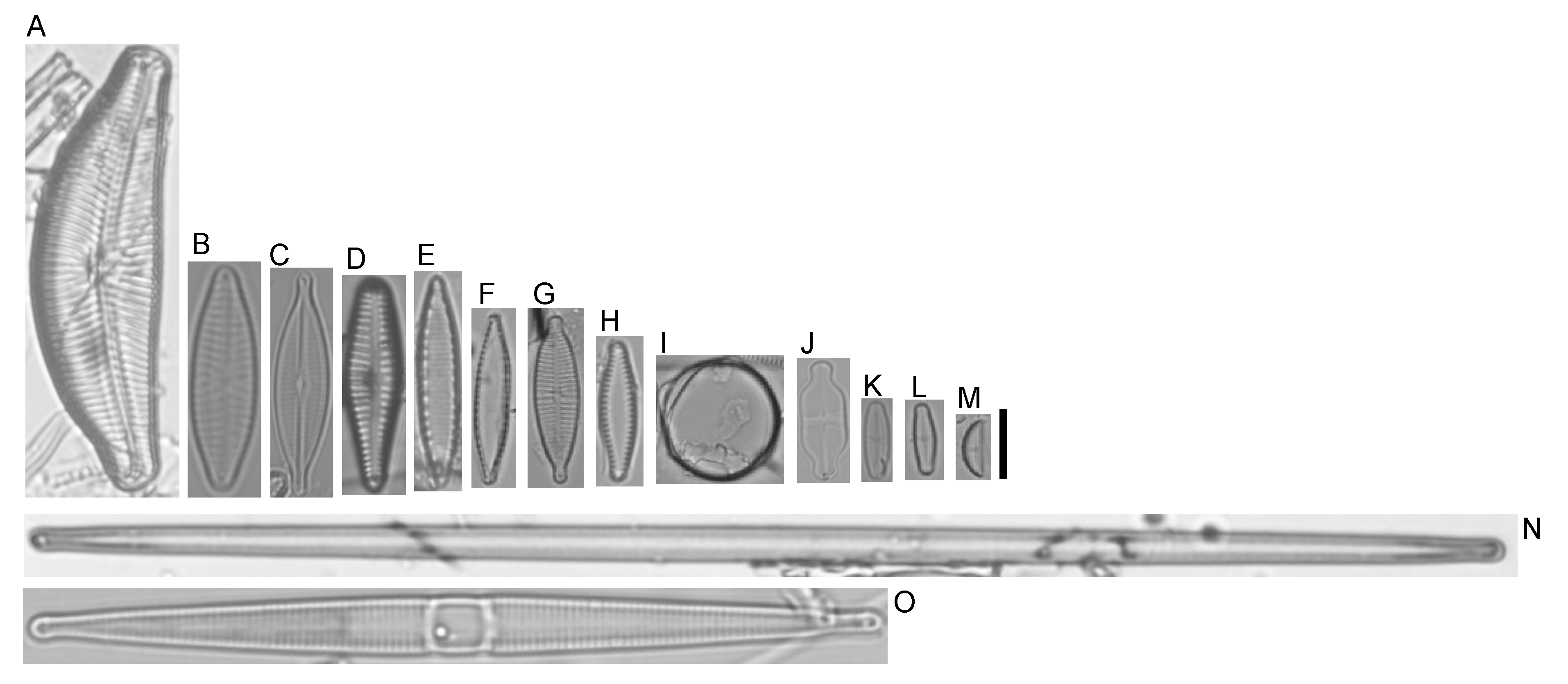
3.1. Diatom Species Identification
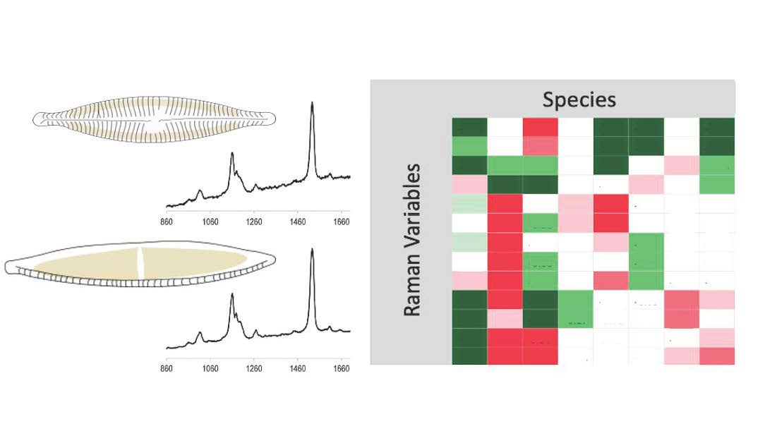
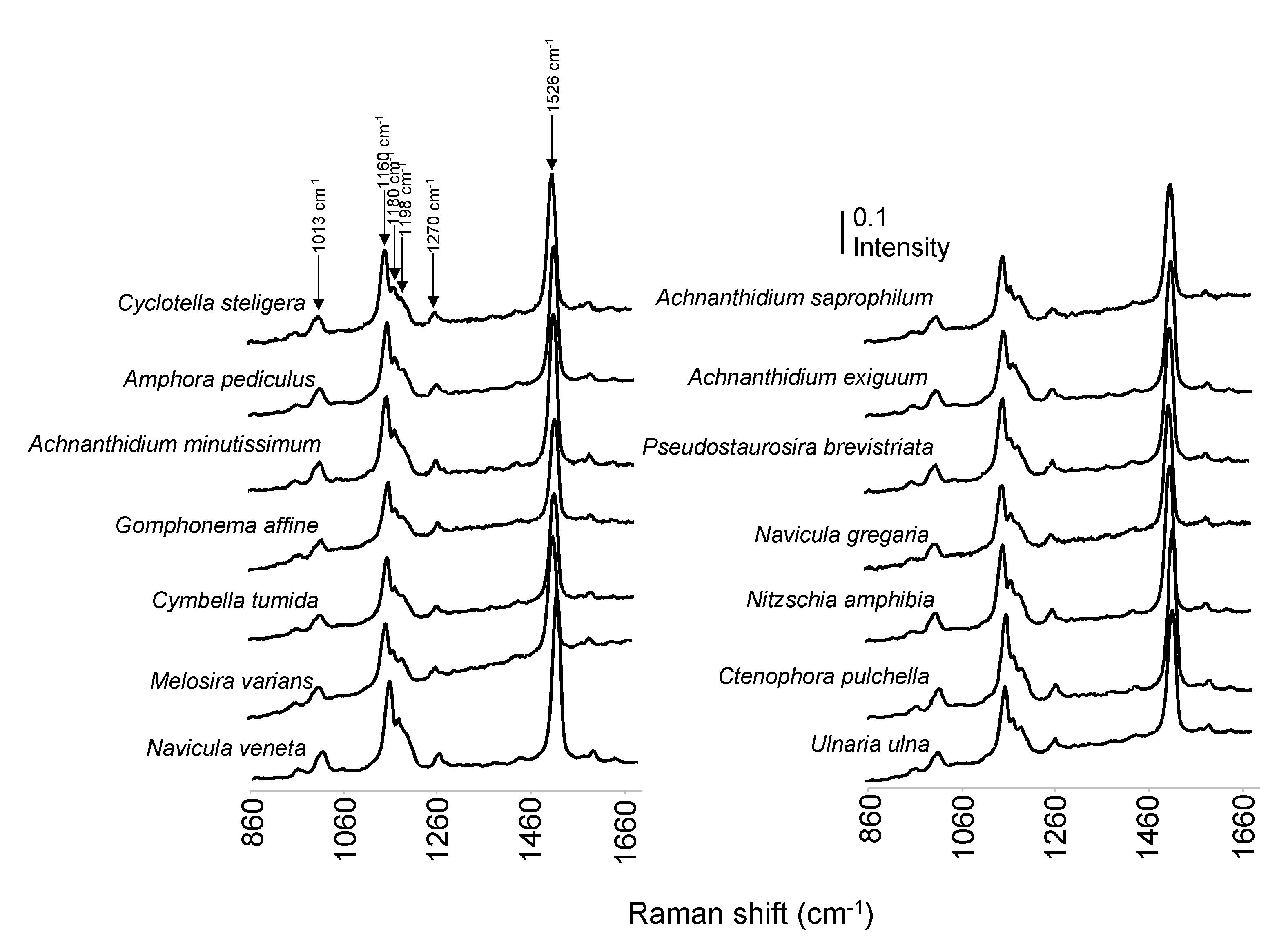
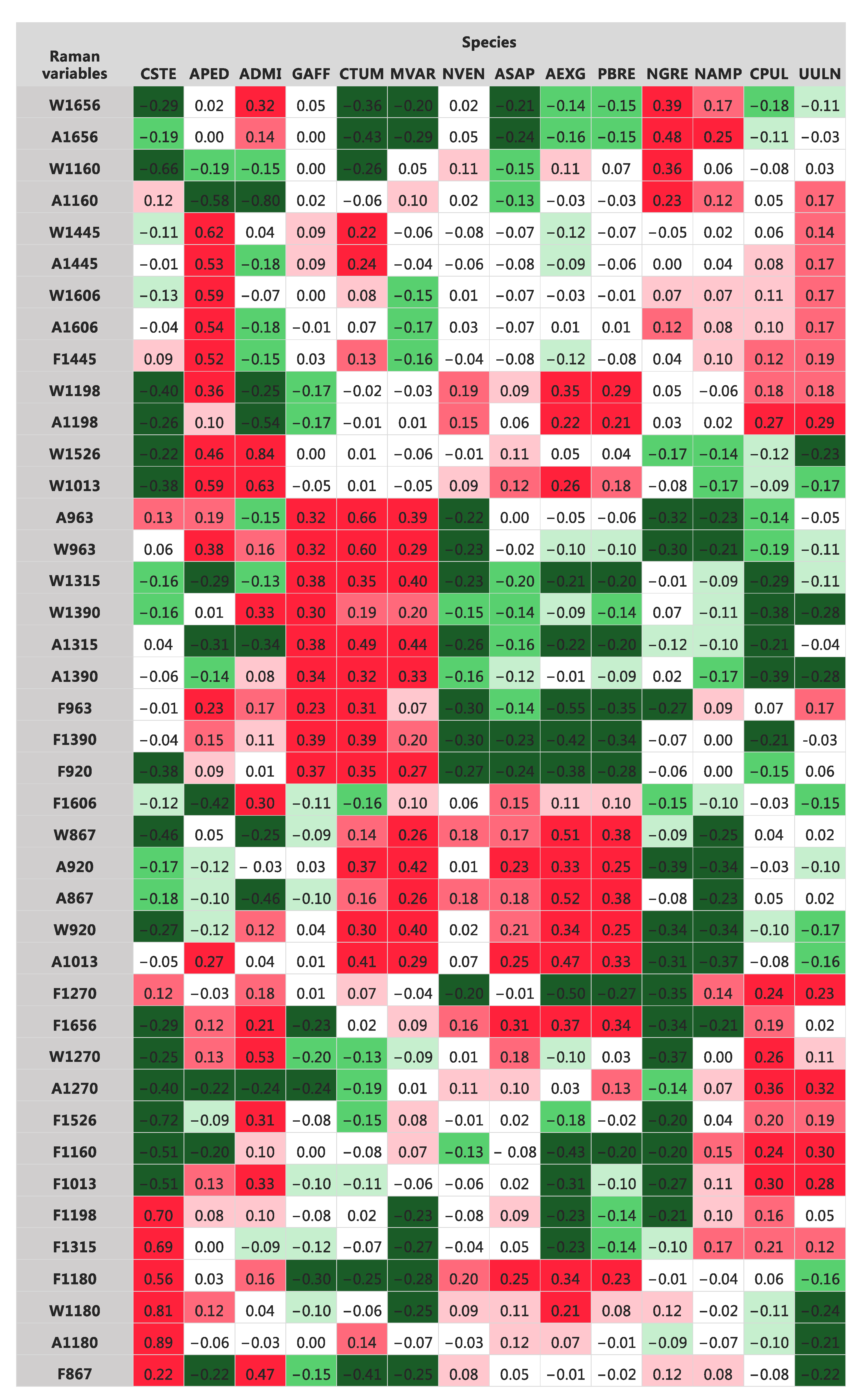
In total, 45 species were identified in all the three sampled lakes. A list of the species found, and respective valve counts is presented in Table S2 (Support information). Of these, 29 species belonging to 15 genera, 12 families, nine orders, and four subclasses showed >1% abundance in at least one lake. The most abundant species were Gomphonema parvulum (Kützing) Kützing, 1849, Melosira varians C. Agardh, 1827, Tabularia tabulata (C.Agardh) Snoeijs, 1992, Achnanthidium minutissimum s.l. (Kützing) Czarnecki, 1994, and Amphora pediculus (Kützing) Grunow ex A. Schmidt, 1875 (Figure 1).

3.2. Raman Spectra

A total of 790 Raman spectra were recorded from all species identified; their number per taxonomic level is indicated in Table 1. All the individuals analysed in this study showed Raman spectra composed by fourteen bands in the 800 to 1660 cm−1 spectral range (Figure 2): located at 867 cm−1, 920 cm−1, 963 cm−1, 1013 cm−1, 1160 cm−1, 1180 cm−1, 1198 cm−1, 1270 cm−1, 1315 cm−1, 1390 cm−1, 1445 cm−1, 1526 cm−1, 1606 cm−1, and 1656 cm−1, respectively. Similar spectra were reported for Thalassiosira pseudonana and Ditylum brightwellii using Ti: sapphire and multimode diode 750 nm lasers as excitation wavelength, 30 mW power, and 30 and 2 s of acquisition time, respectively [45,46]. The Raman signature of the species Cylindrotheca closterium exhibits a similar profile using the 532 nm laser excitation line, a power of 0.1 mW, and an acquisition time of one second [47]. The recorded data was analysed by fitting the sum of damped oscillator functions, and the frequency, band width, and area were obtained for each spectral component. The frequency, band width, and area were the data used in the chemometrics methods.
A PLS-DA regression was done with the data obtained for the species showing >1% abundance to depict their Raman profiles. Six significant components were identified by the PLS-DA. Eleven variables were found to have important contribution to these components (Figure S1, Support Information), which were associated to six different bands: width (W) of the bands at 1526, 1160, 1013, and 1198 cm−1, area (A) of the band at 1160 cm−1 and frequency (F) of the bands at 1526, 1270, 1013, 1180, 1160, and 1198 cm−1. From the band assignments, already available in the literature about Raman applications to diatoms, the bands at 1013, 1160, 1180, and 1526 cm−1 are assigned to C-CH3 in plane rocking modes, as well as C-C, C-H and C=C stretching modes from carotenoids, respectively [28], whereas bands 1198 and 1270 cm−1 can be assigned to N-C and C-N stretching modes of chlorophyll a [28]. It is known that though pigment composition is similar among diatom species, the ratio between the pigments [48], as well as the concentrations of these molecules in different cell compartments, is highly variable [29]. This may explain the differences found among species in the pigment-related bands.
For result interpretation purposes, the scalar projections were calculated (see the methods section). These provided an integrated measure of the relationship (covariance) between the diatom species (Yi) and the Raman variables (Xi) (Figure 3). High positive (red) and High negative (green) scalar projections indicate species showing high positive and negative correlations with the Raman variables, respectively. The Raman module, reflecting the global importance of the descriptors over a given species, was calculated and presented; darker blues representing the highest importance and lighter yellows representing the lowest importance (Figure 3). This integrated analysis allowed us to clearly identify the species best discriminated by the model. In Figure 3, the similarity of species profiles is shown by the cluster analysis. Globally, two main groups of species were easily identified, one with Raman module values ranging from 0.43 to 0.92, representing the species better characterised by the Raman variables, and a second group with notably lower Raman modules. The first group is composed by the species Cyclotella stelligera (Cleve and Grunow) Houk and Klee 2004 (CSTE), Amphora pediculus (APED), Achnanthidium minutissimum (ADMI), Gomphonema affine Kützing, 1844 (GAFF), Cymbella tumida (Brébissoni ex. Kützing) Van Heurck 1880 (CTUM), Melosira varians (MVAR), Navicula veneta Kützing 1844 (NVEN), Achnanthidium saprophilum Kützing 1844 (ASAP), Achnanthidium exiguum (Grunow) Czarnecki, 1994 (AEXG), Pseudostaurosira brevistriata (Grunow) D.M. Williams and Round 1987 (PBRE), Navicula gregaria Donkin 1861 (NGRE), Nitzschia amphibia Grunow 1862 (NAMP), Ctenophora pulchella (Ralfs and Kützing) D.M. Williams and Round 1986 (CPUL), and Ulnaria ulna Compère 2001 (UULN). The relation (covariance) between each Raman variable and each of these species, as derived from the integrated analysis of the six PLS-DA components, is presented in Figure 4. The best characterised species are those represented by darker green and red shades (0–5 and 95–100 percentiles, respectively). Among those are, for example: Cyclotella stelligera (CSTE) (W1160, F1526, F1198, F1315, F1180, W1180, A1180), Amphora pediculus (APED) (A1160, W1445, W1606, A1606, W1013, A1445), Achnanthidium minutissimum (ADMI) (A1160, A1198, W1526, W1013, W1270), Cymbella tumida (CTUM) (A963, W963), and Achnanthidium exiguum (AEXG) (F963).
Variation in the band area assigned to pigments might be related to the amount of these compounds in the cell [47]. For example, the area of band 1160 cm−1 was low for A. minutissimum, a smaller and pioneer taxon capable of colonizing baring substrates and resisting environmental adversities [6]. This indicates low amounts of carotenoids in this species. Among the most important carotenoids in diatoms are fucoxanthin, diadinoxanthin, and diatoxanthin. Fucoxanthin is involved in light-harvesting [48], and diadinoxanthin and diatoxanthin are involved in photoprotection [31,48]. Different band widths might reflect pigment diversity [43]. In contrast to the area, the width of band at 1526 cm−1 showed higher values in A. minutissimum than in the remaining species (Figure 4). This may indicate the presence of a higher variety of carotenoids, which is consistent with the fact that A. minutissimum sensu lato is a species complex encompassing multiple similar species [49]. The band at 1526 cm−1 is a marker of the length of the polyene chain, which vary among different carotenoids [50]. The width of the band 1160 cm−1 was lower in Cyclotella stelligera than in the remaining species (Figure 4), probably reflecting the presence of a lower variety of carotenoids. The frequency of some bands was also relevant to discriminate the species analysed. In particular, the frequency of bands at 1526 cm−1, 1198 cm−1 and 1180 cm−1. In diatom studies, a frequency variation is related to resonance phenomena caused by changes in the wavelength of the incident laser [28,43,51]. Resonance phenomena occur when the energy of the incident laser is similar to the energy of the transition between electrons of a determined compound causing the enhancement of the Raman band corresponding to that compound. Band frequency differences of pigment in solution can also be derived from conformational changes due to the polarity of the solvent [43,51]. In this study, pigments were not extracted, so no solvent was used, and the incident laser frequency was kept constant during the acquisitions. Hence, changes in frequency are most probably due to the presence of different molecular conformations in the measured cells.
Globally, from the results obtained, C. stelligera stood out in profile from the other species. This is a non-motile and planktonic species, contrarily to the other species described [6]. Metabolic and molecular adaptations can occur in this species in response to challenging environmental conditions, which would be reflected in the recorded Raman bands. Overall, interpretation of the PLS by calculation of the scalar projections and Raman modules provided a clear Raman profile characterising each species, also bringing information about their biochemical composition. Future studies should focus on elucidating the differences in molecular conformations that could underlying the frequency shifts recorded in diatom species and the components involved. For example, variation in the components (area, width and frequency) of the bands at 1160, 1180, and 1198 cm−1 can also be assigned to C=S modes of the frustule [52] with previous authors having reported differences among genus in bands related to the frustule components, which may reflect differences in frustule silicification [37].

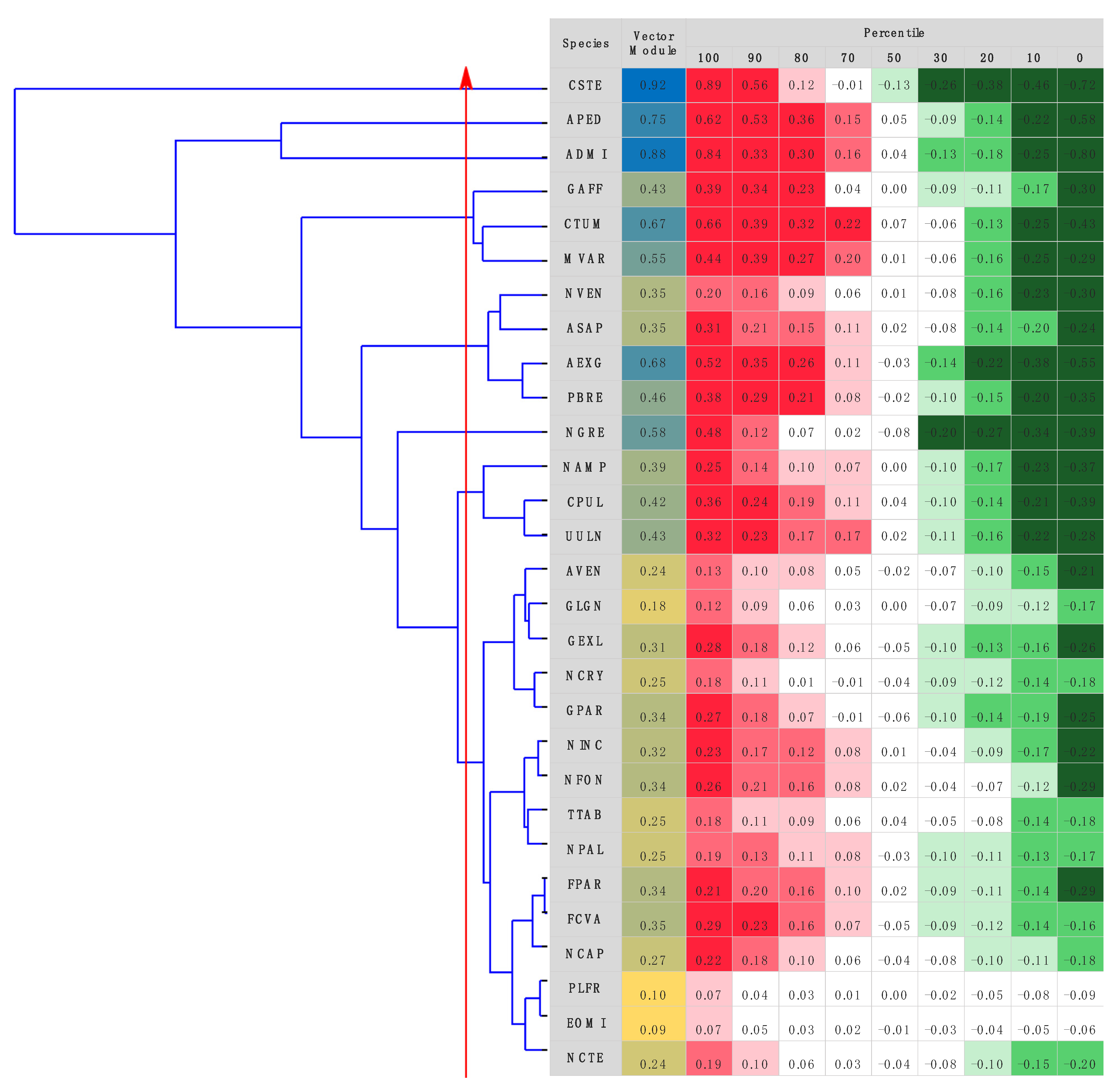
3.3. Taxonomic Identification Using Raman Data

3.3.1. Artificial Neural Network Models

The ANN analysis was carried out with the whole dataset. The best ANN models obtained for the prediction of diatom taxa from Raman data are shown in Table 2. From these results, it is clear that within each subclass, order, and genus, some taxa were predicted with higher performance than others. The ANN methodology showed higher performance in predicting the diatom subclass, returning a prediction with good validation accuracy of 76.0%. The second best model was the one predicting the order (Table 2). It is interesting to note that the lower the number of groups within a given taxonomic level, the higher the classification accuracy obtained. Another possible explanation is that the abundance of taxa could be interfering with the performance of the ANN model [53,54]. Indeed, other authors have found that when a taxon is rare, models tend to learn that the taxon is always absent. Conversely, when a taxon is common, models tend to learn that the taxon is always present [55]. In this work, each species was equally represented in the dataset, independent of their abundance, since the same number of spectra were obtained per species. However, the number of species within higher taxa was not evenly distributed; some taxa contained many species and others only a few. This may be a source of bias in the analysis. Further studies using a more even distribution of species can help clarify this effect and minimize such interferences.
A very relevant aspect of our results is that of the amount of data with which the models were built. Compared to the available literature using ANN for automatic identification of diatoms, the use of Raman data required a remarkably smaller number of samples (spectra in our case). A previous study achieved an excellent accuracy (99.5%) using a total of 160,000 image samples processed by ANN to identify 80 diatom species (2000 samples per species) using a base dataset of 11,000 diatom samples [20]. Libreros and colleagues employed 16,000 segments of 365 images, combined with ANN, to identify diatom genera, achieving a classification accuracy of 74% [57]. A more recent study also using ANN and based on virtual slides obtained through high resolution focus-enhanced light microscopic slide scanning and a series of imaging processing steps, achieved a 95% identification accuracy of four diatom species (Fragilariopsis kerguelensis, Fragilariopsis rhombica, Thalassiosira gracilis, Thalassiosira lentiginosa) and five diatom genera (Asteromphalus, Chaetoceros, Nitzschia, Pseudonitzschia, Rhizosolenia) using a total of 2977 specimens [17]. According to these authors, around 100 specimens per taxon are required for this excellent identification. In another approach, Lambert & Green [58] employed 7092 labelled images processed with ANN to identify ten diatom morphological categories (Centric, Araphid, Symmetrical, Biraphid, Monoraphid, Nitzschioid, Asymmetrical Biraphid, Epithemioid, Surirelloid, Eunotioid) obtained from 1639 species and 112 genus; their accuracy rate was 94%. Finally, a study based on holographic reconstructions from a commercial glass slide containing 50 diatom species achieved an accuracy rate greater than 80% [59]. The authors used an augmented dataset with 174,636 images per class, with a total size of 8,731,800 elements. Overall, these studies showed useful results in the identification of both limited subsets of taxa or larger numbers of genera or species, but always requiring a huge amount of data. They were done with very large imaging datasets involving photographing or scanning and cumbersome pre/pots-processing techniques. Furthermore, most datasets were artificially augmented by imaging processing or segmentation. To the best of our knowledge, this is the first study concerning the prediction of diatom taxa from Raman spectral data. The accuracy rates obtained with a comparatively much lower amount of data, requiring no special processing or preprocessing treatments or artificial augmentation, are very promising, indicating the potential of Raman spectroscopy diatom identification. A more interesting characteristic of these Raman identification models is the high accuracy and sensitivity obtained, relative to the dataset size, when considering that the Raman spectra acquired reflect the biochemical composition of the diatoms rather than their morphological characteristics. Future studies, including species from different geographical locations living under a diverse range of environmental conditions, will provide a sound dataset for ANN and characterisation of Raman profiles for each species, improving species identification.

3.3.2. Species Identification

The model targeting the species was globally the less accurate in the identification (33.7% validation accuracy). However, within this elementary level of taxonomic identification, some species were identified with good sensitivity (Table 3), namely A. minutissimum (80%) and M. varians (82%). Also, the subclass Bacillariophycidae, comprising more than two thirds of the individuals studied (with 556 spectra acquired, see Table 1), was predicted with an excellent sensitivity (89%) by the ANN species model (Table 3). Interestingly, the subclass Thalassiosirophycidae (with only 18 Raman spectra acquired) was predicted with good sensitivity (75%) by this same model (Table 3).
On the whole, the species model is the most important because the species is the basic taxonomic unit. While the accuracy for species determination was lower than expected, the identification of a given organism by an iteration process is one related to hierarchical error. In other words, failing in the identification of a species but not in the identification of its genus is less inaccurate than failing in the identification of both the species and the genus. It is in fact a matter of narrowly failing or failing too close to the target. The same principle is successively applicable up to the subclass level or above. Therefore, decreases in the identification error (1-sensitivity) between taxonomic levels, for example, between the species and its genus, indicate the model is using Raman characteristics, i.e., biochemical characteristics, which are common to the species of that genus, possibly reflecting evolutionarily conserved mechanisms. The concept is particularly interesting as it provides an indication to look for which characteristics are shared by a given taxonomic group that could be established as taxonomic characteristics. Although at the moment the approach is especially useful to complement microscope observations, the fact that taxa identification was still possible over some local variation in conditions points out its promising potential. Raman spectroscopy is very sensitive and able to detect structural molecules useful to distinguish among taxa. This study was a first investigation of the usefulness of this approach in a small area. The next step will be to enlarge the number of sites and ecosystems to refine its use under different environmental and growth conditions and select the most useful Raman spectra to generalise the application.

4. Conclusions

In conclusion, most Raman bands observed in the 800–1660 cm−1 spectral range were found to differ among species and revealed to be useful for their profiling. The integrated interpretation tool derived from the PLS-DA results allowed us to depict a Raman profile for each species that can be used in the characterisation and identification of the different species. The Artificial Neural Network models could better predict the diatom subclasses and order than the species, with accuracy varying from sufficient to excellent (67–89%) using a small dataset of 790 Raman spectra obtained from 29 species, requiring no artificial augmentation. Compared to imaging-based methods, Raman spectroscopy shows high cost-effectiveness in sample measurement and fast acquisition of a great number of variables reflecting the molecular composition of diatoms, with great potential for profiling and detection of characteristics of high taxonomic value.

Supplementary Materials

The following supporting information can be downloaded at: https://www.mdpi.com/article/10.3390/w14132116/s1, Table S1: Mean values (± Standard deviation) of the physical-chemical parameters measured in the three lakes sampled; Table S2: Diatom valve counts and valve percentage found in the three lakes of Oporto’s City Park. Species with the abundance superior to 1% in at least one lake are highlighted; Figure S1. Graphical representation of the most important Raman variables in explaining the variance in the components according to PLS results. The most important variables are highlighted in red: Width (W) of the bands 1526, 1160, 1013 and 1198 cm−1, Area (A) of the band 1160 cm−1 and Frequency (F) of the bands 1526, 1270, 1013, 1180, 1160 and 1198 cm−1.

Author Contributions

R.P., L.G. and L.O.-T. conceived and designed the study; R.P. and L.G. did the diatom sampling; R.P. performed all the analytical measurements; L.O.-T., L.G., R.P., R.V. and J.A.M. performed the statistical analysis of the data; L.O.-T., L.G., R.V., J.A.M. and A.P.C. supervised the research activities carried out; A.P.C. Conceptualization, writing—original draft and review & editing. All authors contributed to the writing of the manuscript, the reviewing and approval of its final version. All authors have read and agreed to the published version of the manuscript.

Funding

This research is a result of the projects REWATER (Water JPI) and BioReset (DivRestore/0004/2020) funded by the BiodivRestore COFUND Action (a joint programme of, BiodivERsA and Water JPI). This research was also supported by national funds through FCT (Portuguese Foundation for the Science and Technology) within the scope of UIDB/04423/2020 and UIDP/04423/2020.

Institutional Review Board Statement

Not applicaple.

Informed Consent Statement

Not applicable.

Data Availability Statement

Not applicable.

Acknowledgments

The authors would like to acknowledge NECL (Network of Extreme Conditions Laboratories), through projects NORTE-01-0145-FEDER-022096 and NORTE-070124-FEDER-000070, for providing the Raman equipment.

Conflicts of Interest

The authors declare no conflict of interest.

References

  1. Round, F.E.; Crawford, R.M.; Mann, D.G. Diatoms: Biology and Morphology of the Genera; Cambridge University Press: Cambridge, UK, 2007. [Google Scholar]
  2. Almeida, S.F.P.; Gil, M.C.P. dÉcologie des diatomées d’eau douce de la région centrale du Portugal. Cryptogam. Algol. 2001, 22, 109–126. [Google Scholar] [CrossRef]
  3. Squires, L.E.; Rushforth, S.R.; Brotherson, J.D. Algal response to a thermal effluent: Study of a power station on the provo river, Utah, USA. Hydrobiologia 1979, 63, 17–32. [Google Scholar] [CrossRef]
  4. Vilbaste, S.; Truu, J. Distribution of benthic diatoms in relation to environmental variables in lowland streams. Hydrobiologia 2003, 493, 81–93. [Google Scholar] [CrossRef]
  5. Rimet, F.; Bouchez, A. Life-forms, cell-sizes and ecological guilds of diatoms in European rivers. Knowl. Manag. Aquat. Ecosyst. 2012, 406, 1. [Google Scholar] [CrossRef]
  6. Lear, G.; Dopheide, A.; Ancion, P.-Y.; Roberts, K.; Washington, V.; Smith, J.; Lewis, G.D. Biofilms in freshwater: Their importance for the maintenance and monitoring of freshwater health. Microb. Biofilms Curr. Res. Appl. 2012, 6700921, 129–151. [Google Scholar]
  7. Mendes, T.; Almeida, S.F.; Feio, M.J. Assessment of rivers using diatoms: Effect of substrate and evaluation method. Fundam. Appl. Limnol. /Arch. Für Hydrobiol. 2012, 179, 267–279. [Google Scholar] [CrossRef]
  8. Feio, M.J.; Hughes, R.M.; Callisto, M.; Nichols, S.J.; Odume, O.N.; Quintella, B.R.; Kuemmerlen, M.; Aguiar, F.C.; Almeida, S.F.; Alonso-EguíaLis, P. The biological assessment and rehabilitation of the world’s rivers: An overview. Water 2021, 13, 371. [Google Scholar] [CrossRef]
  9. Pandey, L.K.; Bergey, E.A.; Lyu, J.; Park, J.; Choi, S.; Lee, H.; Depuydt, S.; Oh, Y.-T.; Lee, S.-M.; Han, T. The use of diatoms in ecotoxicology and bioassessment: Insights, advances and challenges. Water Res. 2017, 118, 39–58. [Google Scholar] [CrossRef]
  10. Pinto, R.; Mortágua, A.; Almeida, S.F.; Serra, S.; Feio, M.J. Diatom size plasticity at regional and global scales. Limnetica 2020, 39, 387–403. [Google Scholar] [CrossRef]
  11. Keck, F.; Vasselon, V.; Tapolczai, K.; Rimet, F.; Bouchez, A. Freshwater biomonitoring in the Information Age. Front. Ecol. Environ. 2017, 15, 266–274. [Google Scholar] [CrossRef]
  12. Morin, S.; Gómez, N.; Tornés, E.; Licursi, M.; Rosebery, J. Benthic diatom monitoring and assessment of freshwater environments: Standard methods and future challenges. In Aquatic Biofilms: Ecology, Water Quality and Wastewater Treatment; Caister Academic Press: Norfolk, UK, 2016; p. 111. [Google Scholar]
  13. Alindonosi, A.; Baeshen, M.; Elsharawy, N. Prospects For Diatoms Identification Using Metagenomics: A Review. Appl. Ecol. Environ. Res. 2021, 19, 4281–4298. [Google Scholar] [CrossRef]
  14. Borrego-Ramos, M.; Bécares, E.; García, P.; Nistal, A.; Blanco, S. Epiphytic diatom-based biomonitoring in Mediterranean ponds: Traditional microscopy versus metabarcoding approaches. Water 2021, 13, 1351. [Google Scholar] [CrossRef]
  15. Coltelli, P.; Barsanti, L.; Evangelista, V.; Frassanito, A.M.; Gualtieri, P. Water monitoring: Automated and real time identification and classification of algae using digital microscopy. Environ. Sci. Processes Impacts 2014, 16, 2656–2665. [Google Scholar] [CrossRef]
  16. Kelly, M.; Juggins, S.; Mann, D.; Sato, S.; Glover, R.; Boonham, N.; Sapp, M.; Lewis, E.; Hany, U.; Kille, P. Development of a novel metric for evaluating diatom assemblages in rivers using DNA metabarcoding. Ecol. Indic. 2020, 118, 106725. [Google Scholar] [CrossRef]
  17. Kloster, M.; Langenkämper, D.; Zurowietz, M.; Beszteri, B.; Nattkemper, T.W. Deep learning-based diatom taxonomy on virtual slides. Sci. Rep. 2020, 10, 1–13. [Google Scholar] [CrossRef]
  18. Mora, D.; Abarca, N.; Proft, S.; Grau, J.H.; Enke, N.; Carmona, J.; Skibbe, O.; Jahn, R.; Zimmermann, J. Morphology and metabarcoding: A test with stream diatoms from Mexico highlights the complementarity of identification methods. Freshw. Sci. 2019, 38, 448–464. [Google Scholar] [CrossRef]
  19. Park, J.; Lee, H.; Park, C.Y.; Hasan, S.; Heo, T.-Y.; Lee, W.H. Algal morphological identification in watersheds for drinking water supply using neural architecture search for convolutional neural network. Water 2019, 11, 1338. [Google Scholar] [CrossRef] [Green Version]
  20. Pedraza, A.; Bueno, G.; Deniz, O.; Ruiz-Santaquiteria, J.; Sanchez, C.; Blanco, S.; Borrego-Ramos, M.; Olenici, A.; Cristobal, G. Lights and pitfalls of convolutional neural networks for diatom identification. In Optics, Photonics, and Digital Technologies for Imaging Applications V; International Society for Optics and Photonic: San Francisco, CA, USA, 2018. [Google Scholar]
  21. Pissaridou, P.; Vasselon, V.; Christou, A.; Chonova, T.; Papatheodoulou, A.; Drakou, K.; Tziortzis, I.; Dörflinger, G.; Rimet, F.; Bouchez, A. Cyprus’ diatom diversity and the association of environmental and anthropogenic influences for ecological assessment of rivers using DNA metabarcoding. Chemosphere 2021, 272, 129814. [Google Scholar] [CrossRef]
  22. Rawat, S.S.; Bisht, A.; Nijhawan, R. A Deep Learning based CNN framework approach for Plankton Classification. In Proceedings of the 2019 Fifth International Conference on Image Information Processing (ICIIP), Shimla, India, 15–17 November 2019; pp. 268–273. [Google Scholar]
  23. Rivera, S.; Vasselon, V.; Jacquet, S.; Bouchez, A.; Ariztegui, D.; Rimet, F. Metabarcoding of lake benthic diatoms: From structure assemblages to ecological assessment. Hydrobiologia 2018, 807, 37–51. [Google Scholar] [CrossRef]
  24. Rivera, S.F.; Vasselon, V.; Ballorain, K.; Carpentier, A.; Wetzel, C.E.; Ector, L.; Bouchez, A.; Rimet, F. DNA metabarcoding and microscopic analyses of sea turtles biofilms: Complementary to understand turtle behavior. PLoS ONE 2018, 13, e0195770. [Google Scholar] [CrossRef]
  25. Salido, J.; Sánchez, C.; Ruiz-Santaquiteria, J.; Cristóbal, G.; Blanco, S.; Bueno, G. A low-cost automated digital microscopy platform for automatic identification of diatoms. Appl. Sci. 2020, 10, 6033. [Google Scholar] [CrossRef]
  26. Selivanova, E.A.; Ignatenko, M.E.; Yatsenko-Stepanova, T.N.; Plotnikov, A.O. Diatom assemblages of the brackish Bolshaya Samoroda River (Russia) studied via light microscopy and DNA metabarcoding. Protistology 2019, 13, 215–235. [Google Scholar] [CrossRef]
  27. Zimmermann, J.; Glöckner, G.; Jahn, R.; Enke, N.; Gemeinholzer, B. Metabarcoding vs. morphological identification to assess diatom diversity in environmental studies. Mol. Ecol. Resour. 2015, 15, 526–542. [Google Scholar] [CrossRef] [PubMed]
  28. Pinto, R.; Vilarinho, R.; Carvalho, A.P.; Moreira, J.A.; Guimaraes, L.; Oliva-Teles, L. Raman spectroscopy applied to diatoms (microalgae, Bacillariophyta): Prospective use in the environmental diagnosis of freshwater ecosystems. Water Res. 2021, 198, 117102. [Google Scholar] [CrossRef] [PubMed]
  29. Heraud, P.; Wood, B.R.; Beardall, J.; McNaughton, D. Probing the Influence of the Environment on Microalgae Using Infrared and Raman Spectroscopy. In New Approaches in Biomedical Spectroscopy; American Chemical Society: Washington, DC, USA, 2007; Volume 963, pp. 85–106. [Google Scholar]
  30. Parker, F.S. Applications of Infrared, Raman, and Resonance Raman Spectroscopy in Biochemistry; Springer Science & Business Media: Berlin/Heidelberg, Germany, 1983. [Google Scholar]
  31. Alexandre, M.T.; Gundermann, K.; Pascal, A.A.; van Grondelle, R.; Buchel, C.; Robert, B. Probing the carotenoid content of intact Cyclotella cells by resonance Raman spectroscopy. Photosynth. Res. 2014, 119, 273–281. [Google Scholar] [CrossRef]
  32. Meksiarun, P.; Spegazzini, N.; Matsui, H.; Nakajima, K.; Matsuda, Y.; Sato, H. In vivo study of lipid accumulation in the microalgae marine diatom Thalassiosira pseudonana using Raman spectroscopy. Appl. Spectrosc. 2015, 69, 45–51. [Google Scholar] [CrossRef]
  33. Rüger, J.; Mondol, A.S.; Schie, I.W.; Popp, J.; Krafft, C. High-throughput screening Raman microspectroscopy for assessment of drug-induced changes in diatom cells. Analyst 2019, 144, 4488–4492. [Google Scholar] [CrossRef] [Green Version]
  34. Pytlik, N.; Klemmed, B.; Machill, S.; Eychmüller, A.; Brunner, E. In vivo uptake of gold nanoparticles by the diatom Stephanopyxis turris. Algal Res. 2019, 39, 101447. [Google Scholar] [CrossRef] [Green Version]
  35. Abbas, A.; Josefson, M.; Abrahamsson, K. Characterization and mapping of carotenoids in the algae Dunaliella and Phaeodactylum using Raman and target orthogonal partial least squares. Chemom. Intell. Lab. Syst. 2011, 107, 174–177. [Google Scholar] [CrossRef]
  36. Wood, B.R.; Heraud, P.; Stojkovic, S.; Morrison, D.; Beardall, J.; McNaughton, D. A portable Raman acoustic levitation spectroscopic system for the identification and environmental monitoring of algal cells. Anal. Chem. 2005, 77, 4955–4961. [Google Scholar] [CrossRef]
  37. Yuan, P.; He, H.P.; Wu, D.Q.; Wang, D.Q.; Chen, L.J. Characterization of diatomaceous silica by Raman spectroscopy. Spectrochim. Acta Part A Mol. Biomol. Spectrosc. 2004, 60, 2941–2945. [Google Scholar] [CrossRef] [Green Version]
  38. Moreira, C.; Gomes, C.; Vasconcelos, V.; Antunes, A. Cyanotoxins occurrence in Portugal: A new report on their recent multiplication. Toxins 2020, 12, 154. [Google Scholar] [CrossRef] [Green Version]
  39. Saker, M.L.; Vale, M.; Kramer, D.; Vasconcelos, V.M. Molecular techniques for the early warning of toxic cyanobacteria blooms in freshwater lakes and rivers. Appl. Microbiol. Biotechnol. 2007, 75, 441–449. [Google Scholar] [CrossRef]
  40. Oliva-Teles, L.; Pinto, R.; Vilarinho, R.; Carvalho, A.P.; Moreira, J.A.; Guimarães, L. Environmental diagnosis with Raman Spectroscopy applied to diatoms. Biosens. Bioelectron. 2022, 198, 113800. [Google Scholar] [CrossRef]
  41. Lange-Bertalot, H.; Hofmann, G.; Werum, M.; Cantonati, M.; Kelly, M. Freshwater Benthic Diatoms of Central Europe: Over 800 Common Species Used in Ecological Assessment; Koeltz Botanical Books: Schmitten-Oberreifenberg, Germany, 2017; Volume 942. [Google Scholar]
  42. Guiry, M.D.; Guiry, G.; AlgaeBase. AlgaeBase; World-Wide Electronic Publication, National University of Ireland, Galway. Available online: https://www.algaebase.org (accessed on 20 May 2020).
  43. Premvardhan, L.; Bordes, L.; Beer, A.; Buchel, C.; Robert, B. Carotenoid structures and environments in trimeric and oligomeric fucoxanthin chlorophyll a/c2 proteins from resonance Raman spectroscopy. J. Phys. Chem. B 2009, 113, 12565–12574. [Google Scholar] [CrossRef]
  44. Oliva Teles, L.; Fernandes, M.; Amorim, J.; Vasconcelos, V. Video-tracking of zebrafish (Danio rerio) as a biological early warning system using two distinct artificial neural networks: Probabilistic neural network (PNN) and self-organizing map (SOM). Aquat. Toxicol. 2015, 165, 241–248. [Google Scholar] [CrossRef]
  45. Meksiarun, P.; Spegazzini, N.; Matsui, H.; Matsuda, Y.; Sato, H. Raman Spectroscopy for Monitoring CO2 Effects on Fatty Acid Synthesis of Microalgal Marine Diatom Thalassiosira pseudonana. Adv. Sci. Eng. Med. 2014, 6, 873–875. [Google Scholar] [CrossRef]
  46. Rüger, J.; Unger, N.; Schie, I.W.; Brunner, E.; Popp, J.; Krafft, C. Assessment of growth phases of the diatom Ditylum brightwellii by FT-IR and Raman spectroscopy. Algal Res. 2016, 19, 246–252. [Google Scholar] [CrossRef]
  47. Pinzaru, S.C.; Müller, C.; Tomšić, S.; Venter, M.M.; Brezestean, I.; Ljubimir, S.; Glamuzina, B. Live diatoms facing Ag nanoparticles: Surface enhanced Raman scattering of bulk cylindrotheca closterium pennate diatoms and of the single cells. RSC Adv. 2016, 6, 42899–42910. [Google Scholar] [CrossRef]
  48. Kuczynska, P.; Jemiola-Rzeminska, M.; Strzalka, K. Photosynthetic pigments in diatoms. Mar. Drugs 2015, 13, 5847–5881. [Google Scholar] [CrossRef]
  49. Novais, M.H.; Juettner, I.; Van de Vijver, B.; Morais, M.M.; Hoffmann, L.; Ector, L. Morphological variability within the Achnanthidium minutissimum species complex (Bacillariophyta): Comparison between the type material of Achnanthes minutissima and related taxa, and new freshwater Achnanthidium species from Portugal. Phytotaxa 2015, 224, 101–139. [Google Scholar] [CrossRef]
  50. Merlin, J.C. Resonance Raman spectroscopy of carotenoids and carotenoid-containing systems. Pure Appl. Chem. 1985, 57, 785–792. [Google Scholar] [CrossRef]
  51. Premvardhan, L.; Robert, B.; Beer, A.; Büchel, C. Pigment organization in fucoxanthin chlorophyll a/c2 proteins (FCP) based on resonance Raman spectroscopy and sequence analysis. Biochim. Biophys. Acta-Bioenerg. 2010, 1797, 1647–1656. [Google Scholar] [CrossRef] [Green Version]
  52. De Tommasi, E.; Congestri, R.; Dardano, P.; De Luca, A.C.; Managò, S.; Rea, I.; De Stefano, M. UV-shielding and wavelength conversion by centric diatom nanopatterned frustules. Sci. Rep. 2018, 8, 1–14. [Google Scholar] [CrossRef]
  53. Dedecker, A.P.; Goethals, P.L.; De Pauw, N. Comparison of artificial neural network (ANN) model development methods for prediction of macroinvertebrate communities in the Zwalm river basin in Flanders, Belgium. Sci. World J. 2002, 2, 96–104. [Google Scholar] [CrossRef] [Green Version]
  54. Manel, S.; Dias, J.-M.; Buckton, S.; Ormerod, S. Alternative methods for predicting species distribution: An illustration with Himalayan river birds. J. Appl. Ecol. 1999, 36, 734–747. [Google Scholar] [CrossRef]
  55. Dedecker, A.P.; Goethals, P.L.; Gabriels, W.; De Pauw, N. Optimization of Artificial Neural Network (ANN) model design for prediction of macroinvertebrates in the Zwalm river basin (Flanders, Belgium). Ecol. Model. 2004, 174, 161–173. [Google Scholar] [CrossRef]
  56. Winter, M.J.; Redfern, W.S.; Hayfield, A.J.; Owen, S.F.; Valentin, J.-P.; Hutchinson, T.H. Validation of a larval zebrafish locomotor assay for assessing the seizure liability of early-stage development drugs. J. Pharmacol. Toxicol. Methods 2008, 57, 176–187. [Google Scholar] [CrossRef]
  57. Libreros, J.; Bueno, G.; Trujillo, M.; Ospina, M. Automated identification and classification of diatoms from water resources. In Iberoamerican Congress on Pattern Recognition; Springer: Berlin/Heidelberg, Germany, 2018; pp. 496–503. [Google Scholar]
  58. Lambert, D.; Green, R. Automatic Identification of Diatom Morphology using Deep Learning. In Proceedings of the 2020 35th International Conference on Image and Vision Computing New Zealand (IVCNZ), Wellington, New Zealand, 25–27 November 2020; pp. 1–7. [Google Scholar]
  59. Memmolo, P.; Carcagnì, P.; Bianco, V.; Merola, F.; Goncalves da Silva Junior, A.; Garcia Goncalves, L.M.; Ferraro, P.; Distante, C. Learning diatoms classification from a dry test slide by holographic microscopy. Sensors 2020, 20, 6353. [Google Scholar] [CrossRef]
Figure 1. Common taxa in the three lakes of Oporto Natural City Park: A—Cymbella tumida; B—Navicula veneta; C—Navicula gregaria; D—Gomphonema gracille; E—Nitzschia amphibia; F—Nitzschia palea; F—Gomphonema parvulum; H—Pseudostaurosira brevistriata; I—Melosira varians; J—Achanthidium exiguum; K—Achnanthidium saprophilum; L—Achnanthidium minutissimum; M—Amphora pediculus; N—Ulnaria ulna; O—Ctenophora pulchella; Scale bar = 10 µm.
Water 14 02116 g001
Figure 2. Raman spectra recorded in the 860 to 1660 cm−1 spectral range from different diatom species. The most important bands identified by the partial least squares discriminant analysis are marked with arrows: 1013 cm−1; 1160 cm−1; 1180 cm−1; 1198 cm−1; 1270 cm−1; 1526 cm−1.
Water 14 02116 g002
Figure 3. Percentiles of the scalar projections, and the Raman module for the integrated importance of the Raman variables over each species were calculated from the six significant components identified by the partial least squares regression discriminant analysis (PLS-DA). Red arrow—Linkage distance cut-off for the determination of the groups in the cluster analysis. High positive (red) and high negative (green) scalar projections indicate taxa showing high positive and negative covariances with the Raman variables, respectively. For the Raman module, darker blues represent the highest importance and lighter yellows represent the lowest importance. The cluster analysis was done on the Y loadings obtained from the PLS-DA. Species are Cyclotella stelligera (CSTE), Amphora pediculus (APED), Achnanthidium minutissimum (ADMI), Gomphonema affine (GAFF), Cymbella tumida (CTUM), Melosira varians (MVAR), Navicula veneta (NVEN), Achnanthidium saprophilum (ASAP), Achnanthidium exiguum (AEXG), Pseudostaurosira brevistriata (PBRE), Navicula gregaria (NGRE), Nitzschia amphibia (NAMP), Ctenophora pulchella (CPUL), Ulnaria ulna (UULN), Amphora veneta (AVEN), Gomphonema lagenula (GLGN), Gomphonema exilissimum (GEXL), Navicula cryptocephala (NCRY), Gomphonema parvulum (GPAR), Nitzschia inconspicua (NINC), Nitzschia fonticola (NFON), Tabularia tabulata (TTAB), Nitzschia palea (NPAL), Fragilaria pararumpens (FPAR), Fragilaria vaucheriae (FCVA), Nitzschia subconstricta (NSBC), Planothidium frequentissimum (PLFR), Eolimna minima (EOMI), Navicula cryptotenella (NCTE).
Water 14 02116 g003
Figure 4. Relationship (covariation) between each Raman variable and each of the best characterised species derived from the integrated analysis (scalar projections) of the six PLS-DA components. Raman variables are represented as width (W), area (A), and frequency (F) of the spectral bands. The colour code indicates the global percentile category of the scalar projections in the whole set. Categories are as follows: dark green, 0–5%; green, 5–10%; light green, 10–20%; pink, 80–90%; red, 90–95%; dark red, 95–100%. The darker the red (positive) or green (negative) tone the greater the effect of the Raman variables over the species. Species legend as in Figure 3.
Water 14 02116 g004
Table 1. Number of Raman spectra collected from each diatom taxonomic level. In total 790 Raman spectra were acquired.
GenusFamilyOrderSubclass
Achnanthidium (72)Achnanthidiaceae (80)Cocconeidales (80)Bacillariophycidae (556)
Planothidium (8)
Amphora (54)Ctenulaceae (54)Thalassiophysales (54)
Cymbella (18)Cymbelaceae (18)Cymbellales (126)
Gomphonema (108)Gomphonemataceae (108)
Nitzschia (162)Bacillariacea (162)Bacillariales (162)
Navicula (126)Naviculaceae (126)Naviculales (134)
Eolimna (8)Sellaphoraceae (8)
Fragilaria (54)Fragilariaceae (54)Fragillariales (72)Fragilariophycidae (162)
Pseudostaurosira (18)Staurosiraceae (18)
Ctenophora (36)Ulnariaceae (90)Licmophorales (90)
Tabularia (36)
Ulnaria (18)
Melosira (54)Melosiraceae (54)Melosirales (54)Melosirophycidae (54)
Cyclotella (18)Stephanodiscaceae (18)Stephanodiscales (18)Thalassiosirophycidae (18)
Table 2. Categorical target, continuous input variables and data set accuracy of the Artificial Neuronal Network (ANN) models with the highest accuracy in the test series. The network architecture used was Multilayer Perceptron (MLP). The accuracy classes considered were those proposed by the European Centre for the Validation of Alternative Methods [56]: sufficient accuracy (65–74%); good accuracy (75–84%); excellent accuracy (>85%).
Categorical TargetSpeciesGenusFamilyOrderSubclass
Continuous inputAllAllAllAllWidth Frequency A1526NN
Train accuracy (%)49.370.174.084.278.3
Test accuracy (%)34.952.654.958.378.9
Validation accuracy (%)34.352.052.653.176.0
Table 3. Validation sensitivity (%) for the taxa best identified by the Artificial Neuronal Network (ANN) using Raman variables as continuous input variables and the species as categorical target. Diatom species, orders, and subclasses with a sensitivity >65% are indicated in bold.
SubclassOrderSpecies
Bacillariophycidae89%Cocconeidales 63%Achnanthidium exiguum 67%
Achnanthidium minutissimum 80%
Thalassiophysales 42%Amphora pediculus 71%
Fragilariophycidae 44%Fragilariales 47%Fragilaria pararumpens 67%
Melosirophycidae 45%Melosirales 64%Melosira varians 82%
Thalassiosirophycidae 75%Stephanodiscales 25%Cyclotella stelligera 50%
Publisher’s Note: MDPI stays neutral with regard to jurisdictional claims in published maps and institutional affiliations.

