Article

ERA5 and ERA-Interim Data Processing for the GlobWat Global Hydrological Model

1
Department Water Resources Management, Faculty of Civil Engineering and Geoscience, Delft University of Technology, 2628 CN Delft, The Netherlands
2
Netherlands eScience Center, 1098 XH Amsterdam, The Netherlands
3
School of Civil Engineering, Iran University of Science and Technology, Tehran 16846-13114, Iran
*
Author to whom correspondence should be addressed.
Water 2022, 14(12), 1950; https://doi.org/10.3390/w14121950
Submission received: 18 May 2022 / Revised: 13 June 2022 / Accepted: 16 June 2022 / Published: 18 June 2022
(This article belongs to the Section Hydrology)

Abstract

:
The reproducibility of computational hydrology is gaining attention among hydrologists. Reproducibility requires open and reusable code and data, allowing users to verify results and process new datasets. The creation of input files for global hydrological models (GHMs) requires complex high-resolution gridded dataset processing, limiting the model’s reproducibility to groups with advanced programming skills. GlobWat is one of these GHMs, which was developed by the Food and Agriculture Organization (FAO) to assess irrigation water use. Although the GlobWat code and sample input data are available, the methods for pre-processing model inputs are not available. Here, we present a set of open-source Python and YAML scripts within the Earth System Model Evaluation Tool (ESMValTool) that provide a formalized technique for developing and processing GlobWat model weather inputs. We demonstrate the use of these scripts with the ERA5 and ERA-Interim datasets from the European Centre for Medium-Range Weather Forecasts (ECMWF). To demonstrate the advantage of using these scripts, we ran the GlobWat model for 30 years for the entire world. The focus of the evaluation was on the Urmia Lake Basin in Iran. The validation of the model against the observed discharge in this basin showed that the combination of ERA5 and the De Bruin reference evaporation method yields the best GlobWat performance. Moreover, the scripts allowed us to examine the causes behind the differences in model outcomes.

1. Introduction

The reproducibility of computational hydrology is gaining attention among hydrologists [1,2,3,4,5,6]. Several definitions of reproducibility have been proposed. The concept of these definitions includes access to all data, models, code, and the research environment. Access must be such that a new user can precisely reproduce the results given by the main study and that a set of new data can also be processed [7,8]. Nevertheless, a recent study showed that, on average, only 1.1% of the publications in hydrology and water resources are fully reproducible [8]. This is because most researchers either do not share their code and data or, when they do, the details and dependencies are omitted [9]. Reproducibility is important to validate previous results and to advance earlier research [10].
Global hydrological models (GHMs) are rapidly evolving as a result of developments in computational capacity and data storage as well as developments in remote sensing, the availability of gridded observation datasets, and meteorological forcing data [11]. Creating input files for GHMs becomes exceedingly challenging as their resolution improves [12]. Each GHM reads input data in a specific format. As a result, raw gridded datasets have to be pre-processed before being used by a GHM. These modifications require programming and technical skills that are often not available among hydrologists. Recently, steps have been taken to address the lack of data sharing in hydrology, break the knowledge barrier for data processing, and reduce the time required for data processing. Journals now request that authors submit their model code and data [7]. However, the scripts or software used to process the input data are rarely published alongside the papers [1]. Several platforms have been developed to make hydrological models and data findable, accessible, interoperable, and reproducible (FAIR) [13]. Hydroshare [14] provides services for data sharing. The data are published without any scripts or tools for their processing, and researchers must process the data for their applications. HydroDS [15] offers a web service powered by a Python workflow that allows users to request and download data in a model-friendly format. eWaterCycle [5] offers a reproducible model software environment as well as input data processing for their supported models. Despite numerous efforts to provide data and input data processing for hydrological models, not all GHMs are supported by the current platforms. As a result, input data pre-processing for these models is critical to providing FAIR hydrological models that researchers around the world can use in new case studies.
None of the previous efforts provided input processing scripts for the FAO’s GlobWat model [16]. GlobWat is a high-resolution GHM designed to estimate current and future water consumption by agriculture, the world’s largest water consumer. The GlobWat model uses gridded precipitation and reference evaporation (Eref) in ASCII format as the weather input. The model code and sample input data can be found on the FAO’s AquaMaps website [17]. The methods for creating and processing model inputs, however, have not been established, limiting the model’s reproducibility and reusability. In this paper, a new set of open-source Python and YAML scripts is created within the Earth System Model Evaluation Tool (ESMValTool) [18], which provides a formalized method for pre-processing weather input datasets. Although these scripts are designed to generate readable GlobWat input data formats from ERA5 and ERA-Interim, they can be adapted and reused to generate readable GlobWat weather input data from other ESMValTool-supported datasets [19], such as the Climate Research Unit (CRU) dataset. Many of the time-consuming and complex processes, such as downloading and standardizing raw data, calculating reference evaporation, unit conversion, re-gridding, and generating a readable GlobWat format, are automated by the developed scripts.
GHMs’ climate inputs are commonly gridded climate datasets [20,21]. Gridded climate datasets known as atmospheric reanalysis data are commonly used. In a dynamical–physical coupled numerical model, reanalysis data are produced by combining a variety of measured and remotely sensed data. Atmospheric reanalysis at various spatial and temporal scales is now available from several modeling centers [22,23]. The National Center for Atmospheric Research (NCAR) recommends that reanalysis variables related to the hydrological cycle, such as precipitation and evaporation, should be used with extreme caution. The accuracy of reanalysis can differ considerably depending on the location, time period, and variable selected [24]. The European Centre for Medium-Range Weather Forecasts (ECMWF) is one of the modeling centers that produces reanalysis datasets. This center developed atmospheric datasets, including ERA-Interim and the latest released ERA5. ERA5 and ERA-Interim are increasingly used in hydrological modelling [22,25,26,27]. ERA5 outperforms ERA-Interim in several aspects, such as higher temporal and vertical resolution, and has replaced ERA-Interim [28,29]. However, it is not clear how these improvements will affect hydrological modeling. For instance, Tarek et al. [22] found that ERA5 and ERA-Interim performed similarly in the estimation of temperature in North America, and the improvement in hydrological modeling over North America using ERA5 was not related to the ERA5’s improved resolution. Thus, it is essential to assess ERA5 performance in hydrological modelling and document ERA5’s improvements over ERA-Interim. Accordingly, in this study, ERA5 and ERA-Interim datasets were selected as the climate datasets to be processed for the GlobWat model.
The main objectives of the current study are to (1) provide open-source Python and YAML scripts to process ERA5 and ERA-Interim data provided by the ECMWF for use in GlobWat; (2) run the GlobWat model using processed data for the 30 years from 1986 to 2016; (3) assess GlobWat model performance in the Urmia Lake Basin, Iran, using observed discharge; (4) an evaluation of the ERA5 and ERA-Interim datasets for hydrological modeling with GlobWat; and (5) an evaluation of the De Bruin and Langbein method for calculating Eref and a comparison with ERA5 Eref.

2. Materials and Methods

2.1. The GlobWat Model

The GlobWat model is a GHM that has been developed by the FAO to evaluate water consumption in irrigated agriculture. The GlobWat input layers are the monthly precipitation, the number of wet days per month, the coefficient of variation of precipitation, the monthly Eref, the maximum soil moisture storage capacity, the maximum groundwater recharge flux, irrigated areas, land use, and areas of open water and wetlands. The input variables of the model are the monthly precipitation and Eref. The other layers are predefined and provided by the model developers from various sources [30,31,32,33,34,35]. The GlobWat input layers and their sources are listed in the Table A1 of Appendix A. The water balance in GlobWat is calculated in two steps. The first step is a vertical water balance to calculate rain-fed evaporation, which has a daily time step. The second step is a horizontal water balance for surface water, which has a monthly time step [16]. GlobWat has a spatial resolution of approximately 10 km and reads layers in ASCII format. The grid specification for GlobWat is shown in Table 1.

2.2. Eref Methods and Data Processing

In this study, we provide a recipe (a YAML script) and a diagnostic (a Python script) for processing precipitation and Eref for use in the GlobWat hydrological model. The recipe is used to specify the input data required by the diagnostic as well as to set optional processing. The diagnostic is where calculations related to Eref are performed, and necessary changes are made to the data in the format used in the model.
The recipe and diagnostic were developed within the ESMValTool. The ESMValTool is a community-based open-source software package for the comprehensive analysis of Earth system models (ESMs) [18]. To assess the performance of a model, the ESMValTool uses both diagnostics and performance metrics. The ESMValTool has preprocessing functions for adjusting the data before applying diagnostics or metrics. The ESMValTool’s most typical data adjustments are the calculation of non-directly available variables, vertical interpolation, land–sea or ice masking, re-gridding, multi-model statistics, temporal and spatial manipulations, missing value masking, and unit conversion [37].
Section 2.2.1 and Section 2.2.2 describe the Eref method used in this study as well as the token processing steps.

2.2.1. Eref Methods

Eref is an ERA5 parameter described in the ECMWF parameter details [38]. However, Eref is not included in ERA-Interim. In addition to Eref from ERA5, we calculated the Eref for ERA5 and ERA-Interim. Eref at the global scale for use in GlobWat can be calculated based on the De Bruin and Langbein methods.

De Bruin Method

The De Bruin method is a straightforward algorithm that uses a thermodynamic technique to calculate the Eref of a well-watered grass field that closely resembles the FAO reference grass. This method calculates Eref as a function of the two-meter air temperature, mean sea level pressure, surface solar radiation downwards, and top of atmosphere (TOA) incident solar radiation. The results of the De Bruin method have been validated using Cabauw in situ observations in the Netherlands [39]. A python script has been provided for the calculation of Eref using the De Bruin method in the ESMValTool [40] and the eWaterCycle [41].

Langbein Method

The Langbein method to calculate Eref is an empirical relationship between the average annual temperature and Eref, based on data from 20 catchments across the United States. These catchments vary from humid to arid and from cold to warm [42,43]. This equation has been used in Eref analyses in various regions, including arid, semi-arid, and humid regions [44,45,46,47,48]. The Langbein calculation is shown in Equation (1), where Eref is in mm and T is the average annual temperature in °C.
Eref   =   325 + 21   ×   T   +   0.9   ×   T 2
The Langbein method has been added to the ESMValTool to address the interests of researchers who intend to use or have used this method and want to compare their results with ERA5 and ERA-Interim. The Langbein temperature-based Eref method is mainly useful in those basins where only the observed temperature is available. ERA5, ERA-Interim, and GlobWat operate at a global scale, allowing researchers to choose any location for further assessments.

2.2.2. Processing Steps

We provided a recipe [49] and a diagnostic [50] for processing the precipitation and Eref for use in the GlobWat model. The GlobWat recipe includes monthly and daily data processing of the ERA5 and ERA-Interim datasets. When the ESMValTool runs the GlobWat recipe, it finds the data and runs the processing function. It also executes the diagnostic script that involves a GlobWat-specific analysis to extract Eref and the precipitation, and stores the provenance details to ensure transparency and reproducibility. The processing flowchart is shown in Figure 1a.
In this paper, we use monthly data. However, the recipe can be run using daily data as well. The download and CMORization (Climate Model Output Rewriter) of input data are the first steps of data processing. The script to download ERA-Interim data is available at the ESMValTool GitHub repository [51], and ERA5 can be downloaded using era5cli [52].
CMORization is the process of standardizing data to ensure that it is CF (climate and forecast) compliant and follows the CMOR tables (standard_name, units, long_name, etc) [5,34]. For example, the ERA-Interim CMORizer changes the precipitation units from meters of water per day to kg of water per m2 per day, converts the ERA-Interim 6 hr frequency to daily, and sets standard names for variables. The ERA-Interim and ERA5 CMORizer Python scripts can be found in the ESMValTool GitHub repository [53,54].
CMORization is performed only once for each dataset. The CMORized data can then be used in any ESMValTool recipe. Our recipe uses the CMORized ERA5-daily/monthly and ERA-Interim-daily/-monthly data. Then, Eref is calculated based on the De Bruin or Langbein methods.
Another variable required by GlobWat is precipitation, which is available in both datasets. However, the interpolation of cumulative precipitation fields often results in negative values [55]. To prevent NaN values in the GlobWat outputs, these negative values are set to zero. Next, a unit conversion is applied to both the precipitation and Eref to convert units from kg m−2s−1 to mm per time step (month or day).
Subsequently, to match the grid size of the datasets with that of the GlobWat model, re-gridding is performed. The re-gridding scheme is set to ‘area weighted’ to keep the volume of water consistent before and after re-gridding. In this method, the data for each target grid are generated as a weighted mean of all cells from the source grid.
Finally, the data are saved in ASCII format and are ready for use as inputs in the GlobWat model. An example of processing ERA-Interim precipitation for the year 2004 for January is presented in Figure 1b.
We provide more details about the scripts on the ESMValTool documentation page [56].

2.3. Data

2.3.1. ERA5 and ERA-Interim

ERA5 and ERA-Interim are global atmospheric reanalysis datasets provided by the ECMWF [28,57]. ERA-Interim covers January 1979 to 31 August 2019, and ERA5 covers January 1950 to the present [29,58]. ERA5 and ERA-Interim have spatial resolutions of 30 km and 79 km and temporal resolutions of 1 hour and 6 hours, respectively [29]. Details about the ERA5 and ERA-Interim datasets can be found on the ECMWF website [59,60]. ERA-Interim and ERA5 are often used for hydrological modeling [4,5]. Recently, the impact of ERA5 over ERA-Interim for use in hydrological models has been studied [4,5,22,61]. We retrieved the precipitation, two-meter air temperature, mean sea level pressure, surface solar radiation downwards, and top of atmosphere (TOA) incident solar radiation from 1986 to 2016.

2.3.2. Observed Hydro-Climatic Variables

The observational data were obtained from D. Moshir Panahi et al. [62]. They gathered data from synoptic meteorological stations for precipitation (P) and temperature as well as discharge (Q) data from hydrometric stations in the Urmia Lake Basin. The annual basin precipitation and temperature were estimated using Thiessen polygons, also using synoptic stations from neighboring basins to obtain precise estimations. The annual discharge was calculated by dividing the measured discharge values by the corresponding basin area. Water storage changes (DS) were determined based on the groundwater storage in the aquifer below the basin. There was no direct measurement of the actual evaporation (Eact) at the basin scale. Therefore, they calculated Eact from the measured P, Q, and DS and a water balance equation:
Eact = P − Q − DS

2.4. The Urmia Lake Basin, an Example Case Study

The Urmia Lake Basin is located in northwestern Iran. The elevation of the Urmia Lake Basin varies between 1204 and 3804 m. It has been classified as a biosphere reserve by UNESCO [63,64]. Urmia Lake is the world’s second-largest hypersaline endorheic lake [65]. Rain-fed agriculture and manufacturing are the two main economic sectors in the Urmia Lake Basin, which is home to more than 6.5 million people [66]. Figure 2 depicts the locations of the Urmia Lake Basin. The area of the basin is 51,440 km2 [67]. The Urmia Lake Basin, with a mean annual temperature of 12 °C and precipitation of 303 mm/yr, has a cold and semi-arid climate [67,68].

2.5. Evaluation Statistics

Four statistics were used in the assessment to evaluate the ERA5/ERA-Interim precipitation and observed precipitation and the performance of the GlobWat model in estimating the observed discharge over the Urmia Lake Basin during the modeling period. The statistics include the correlation coefficient (CC), standard deviation (SD), root-mean-square error (RMSE), and Nash–Sutcliffe efficiency (NSE), which are defined as follows:

2.5.1. Correlation Coefficient (CC)

Equation (3) gives the correlation coefficient between the observed values and those estimated by GlobWat (Q and Eact) or datasets (ERA5/ERA-Interim P and T); it ranges from −1 to 1.
CC = Cov   ( Y est Y obs ) Var   ( Y est ) Var   ( Y obs )
Here, Y est is a variable estimated by GlobWat or a dataset variable, and   Y obs is the observed variable. The closer R is to one, the better the model reproduces the observed variability.

2.5.2. Standard Deviation (SD)

The standard deviation is a measure of how far values deviate from the mean. The standard deviation is calculated as the square root of the sum of the squared differences from the mean divided by the size of the dataset (Equation (4)).
SD = i = 1 n ( Y i     Y ¯ ) 2 n

2.5.3. Root-Mean-Square Error (RMSE)

The RMSE, which ranges from 0 to infinity and expresses how close the model’s estimation or dataset variable is to the observed variable, is calculated with Equation (5).
RMSE = i = 1 n ( Y obs , i   Y est , i ) 2
The closer the RMSE gets to 0, the more accurate the model’s estimate or dataset value is.

2.5.4. Nash–Sutcliffe Efficiency (NSE)

The NSE is described by Equation (6) and ranges from -infinity to 1.
NSE = 1   i = 1 n ( Q obs ,   i   Q est , i ) 2 i = 1 n ( Q obs , i   Q obs ¯ ) 2
Here, Q obs , i is the observed discharge, and   Q est , i is the estimated discharge by the model. NSE = 1 indicates that the estimated discharge is consistent with the observed discharge and a negative NSE states that the mean of the observed discharge is a better predictor than the model.

3. Results

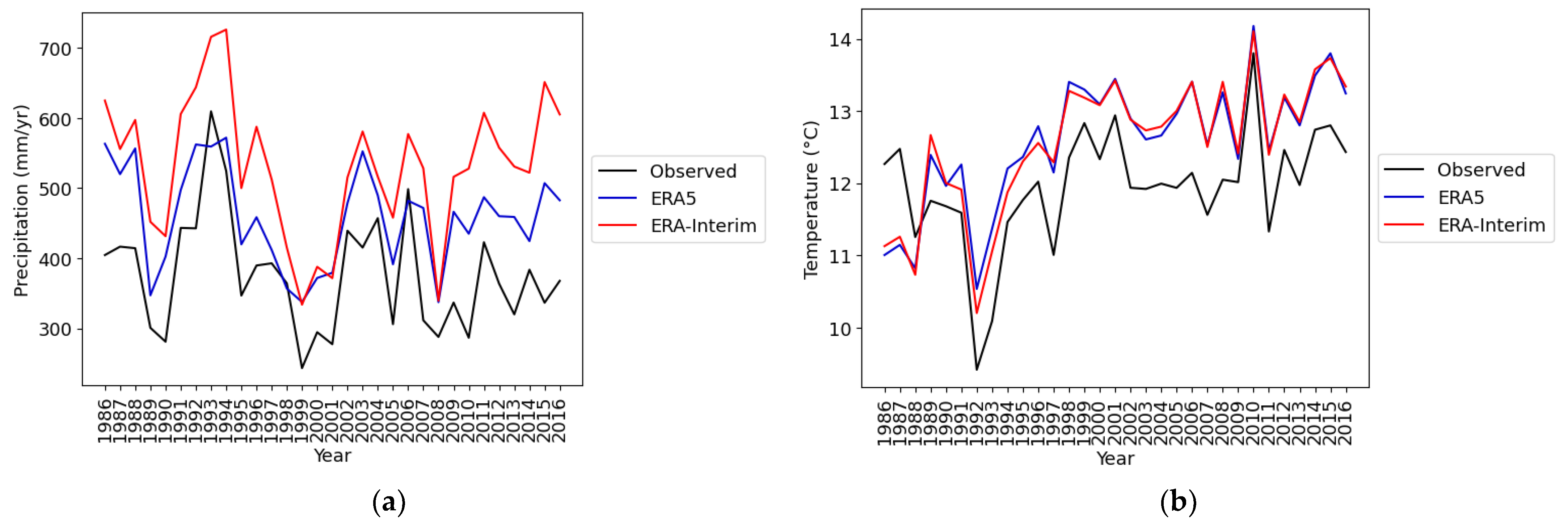
We compared the precipitation and temperature estimates for our study period (1986–2016) from the ERA5 and ERA-Interim datasets to observations from the Urmia Lake Basin. Figure 3 shows a comparison of the ERA5 and ERA-Interim precipitation and temperature values with the observed values. ERA5 and ERA-Interim overestimated precipitation and temperature over the Urmia Lake Basin. ERA5 overestimated precipitation less than ERA-Interim. While both datasets had similar temperature estimates. The patterns of the ERA5 and ERA-Interim datasets resembled that of the observation data, and in many cases, the observed precipitation and temperature increases and decreases were consistent with the ERA5 and ERA-Interim precipitation and temperature. However, the precipitation estimates from ERA5 and ERA-Interim from 2006 to 2016 deviated more significantly from the observed data. As a result, we examined three periods in our analysis to better understand the impact of this deviation on GlobWat’s discharge estimations. These periods were 1986–2016, 1986–2006, and 2006–2016.
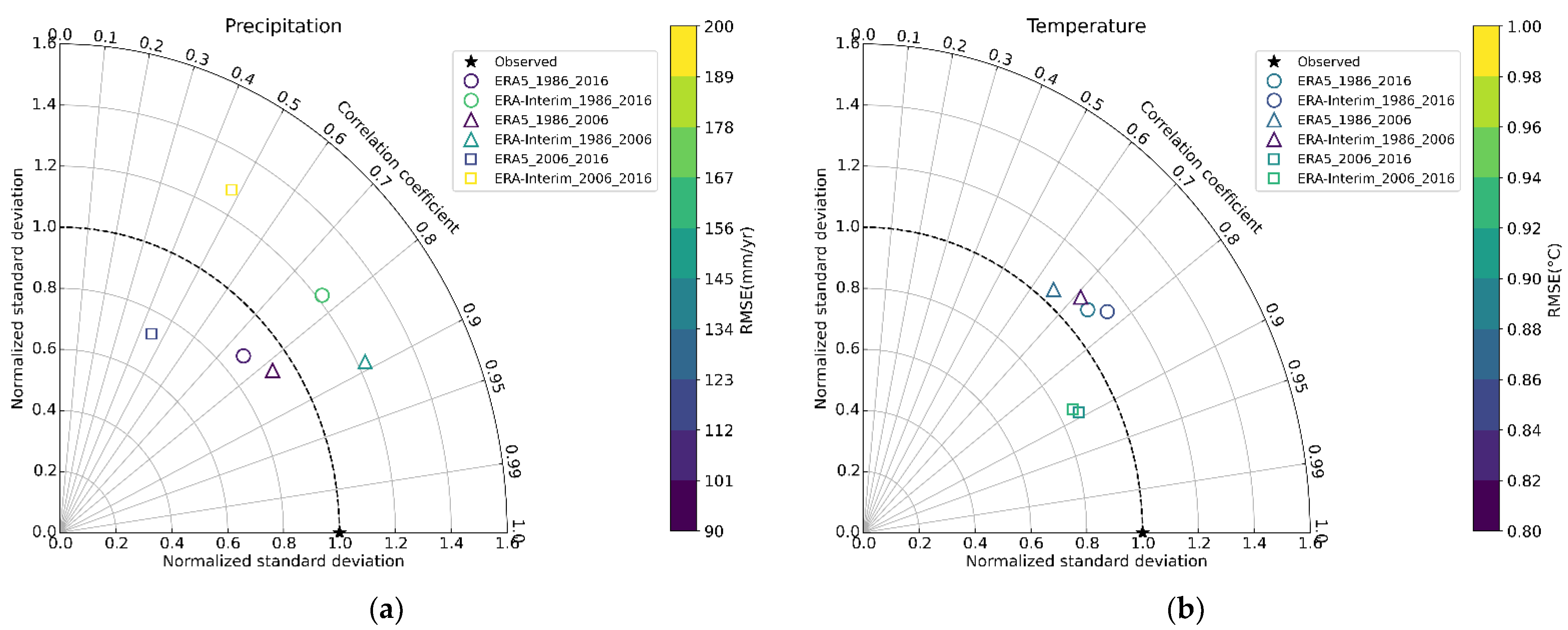
The Taylor diagram, which is based on the CC, normalized SD (NSD), and RMSE, provides a graphical summary of the agreement between the observed and estimated data [69]. In order to display multiple periods in a single figure, the standard deviations of the reference datasets were normalized to 1.0 based on the observed standard deviations. The closer a dataset is to the black star marker, the more accurate the estimated data are. Figure 4 shows that the ERA5 and ERA-Interim datasets performed relatively well in estimating the precipitation and temperature for the time periods of 1986–2006 and 1986–2016. However, ERA5 and ERA-Interim had the lowest agreement in representing precipitation from 2006 to 2016. The datasets performed equally well for the estimation of temperature in all periods, while ERA5 performed better than ERA-Interim regarding precipitation. For the period of 1986–2006, the precipitation was slightly better represented in both ERA5 and ERA-Interim compared to 1986–2016 by having lower RMSEs, whereas in the period of 2006–2016, ERA5 and ERA-Interim precipitation was not well presented and had the highest RMSEs. In general, the ERA5 and ERA-Interim temperatures had the same performance in all periods by having almost equal RMSEs. Tables S1 and S2 in the Supplementary Materials show the CCs, SDs, NSDs, and RMSEs for the ERA5 and ERA-Interim precipitations and temperatures against the observed data. The statistics were calculated for the periods of 1986–2016, 1986–2006, and 2006–2016.
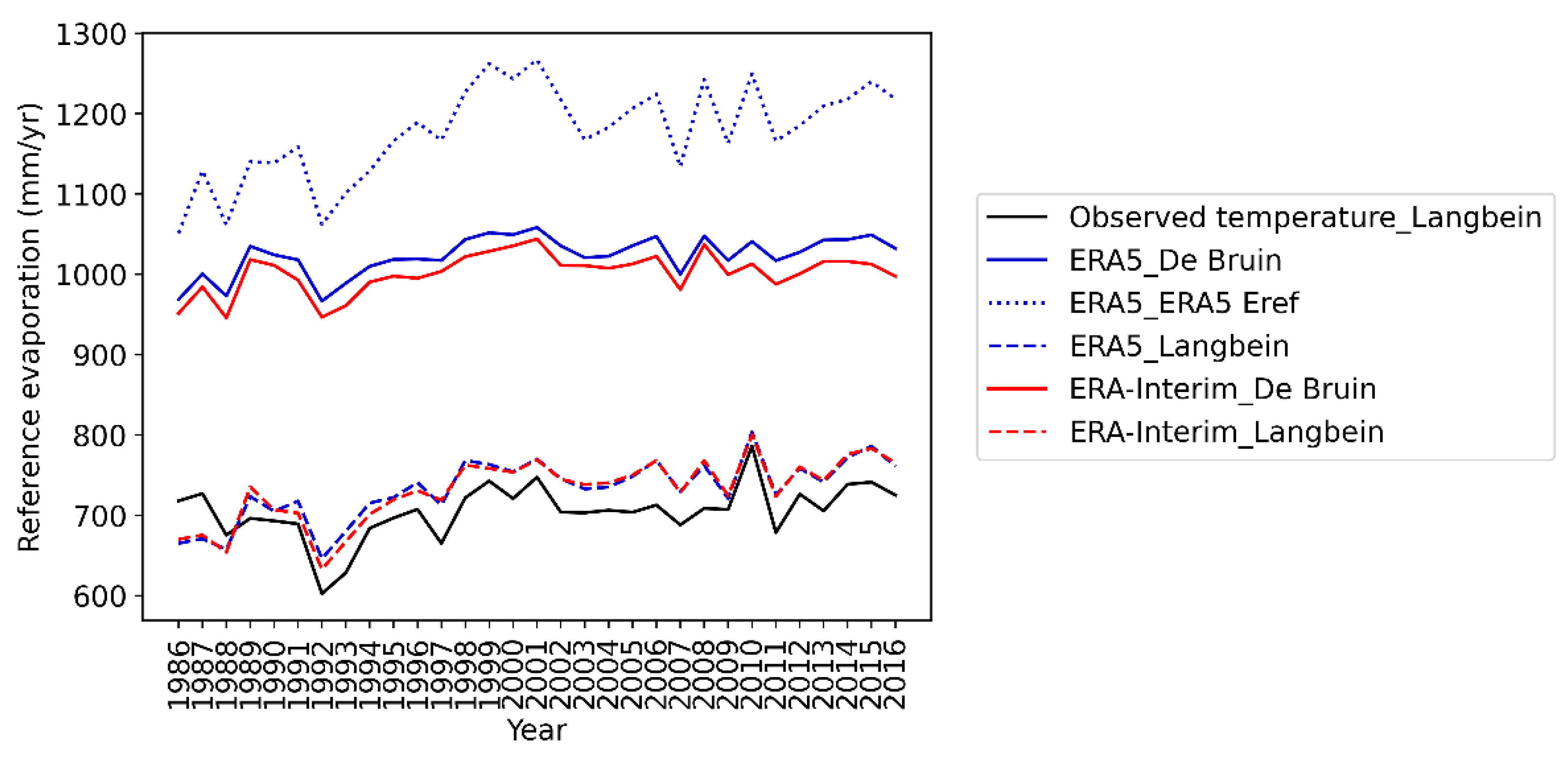
We calculated Eref for use in the GlobWat model with the ERA5, ERA-Interim, and observed datasets using the De Bruin and Langbein methods. Since the ERA5 dataset contains Eref, we also retrieved Eref from the ERA5 dataset. Figure 5 depicts the calculated Eref values and the Eref retrieved from ERA5. In comparison to the Eref calculated using the De Bruin and Langbein methods, the ERA5 Eref had the highest values of Eref for the Urmia Lake Basin. However, it resembled the Eref patterns calculated by the De Bruin and Langbein methods.
In general, the method used to calculate the Eref appears to have a greater effect on the generated Eref values than the datasets used for the calculations. For example, the Eref values calculated using the De Bruin method with ERA5 and ERA-Interim were close to each other. Accordingly, the Eref estimates using the Langbein method were also close. Due to the lack of observed data, the Langbein method was used to compute Eref because it only requires observed temperature.
The GlobWat model was used to estimate the discharge and Eact for each basin of the world for 30 years, from 1986 to 2016. GlobWat was run five times with various Eref methods and reanalysis products each time. The runs included ERA5 in combination with different Eref methods, including De Bruin, Langbein, and the Eref retrieved from the ERA5 dataset (ERA5 Eref). Additional runs included ERA-Interim with combinations of the De Bruin and Langbein Eref methods. The GlobWat-model-developed scripts for downloading and processing the ERA5 and ERA-Interim for use in GlobWat, as well as their documentation, are accessible online. Appendix B describes the steps and online resources required to run the GlobWat model using the scripts developed in this study.
GlobWat produces results for each of the world’s major basins. In this study, we analyzed the results calculated for the Urmia Lake Basin. Figure 6 shows a comparison between the estimated discharges using the De Bruin and Langbein methods. For the whole study period, in many cases, the estimated discharge patterns closely resembled that of the observation data. The estimated discharge represents the same downward trend as the observed discharge.
To compare the estimated and observed discharge at the Urmia Lake Basin over time, we used a Taylor diagram together with the RMSE and NSE to evaluate the GlobWat model performance. Figure 7 shows that the model had similar performances during 1986–2016 and 1986–2006. However, the model’s performance in representing the discharge was lower from 2006 to 2016. In all periods, the model’s performance using the ERA5 weather dataset and the De Bruin Eref method was the best, with the highest values of NSE and lowest values of RMSE. The statistical values between the observed and estimated discharge by GlobWat are shown in Table S3 of the Supplementary Materials (e.g. CC, SD, NSDs, and RMSE).
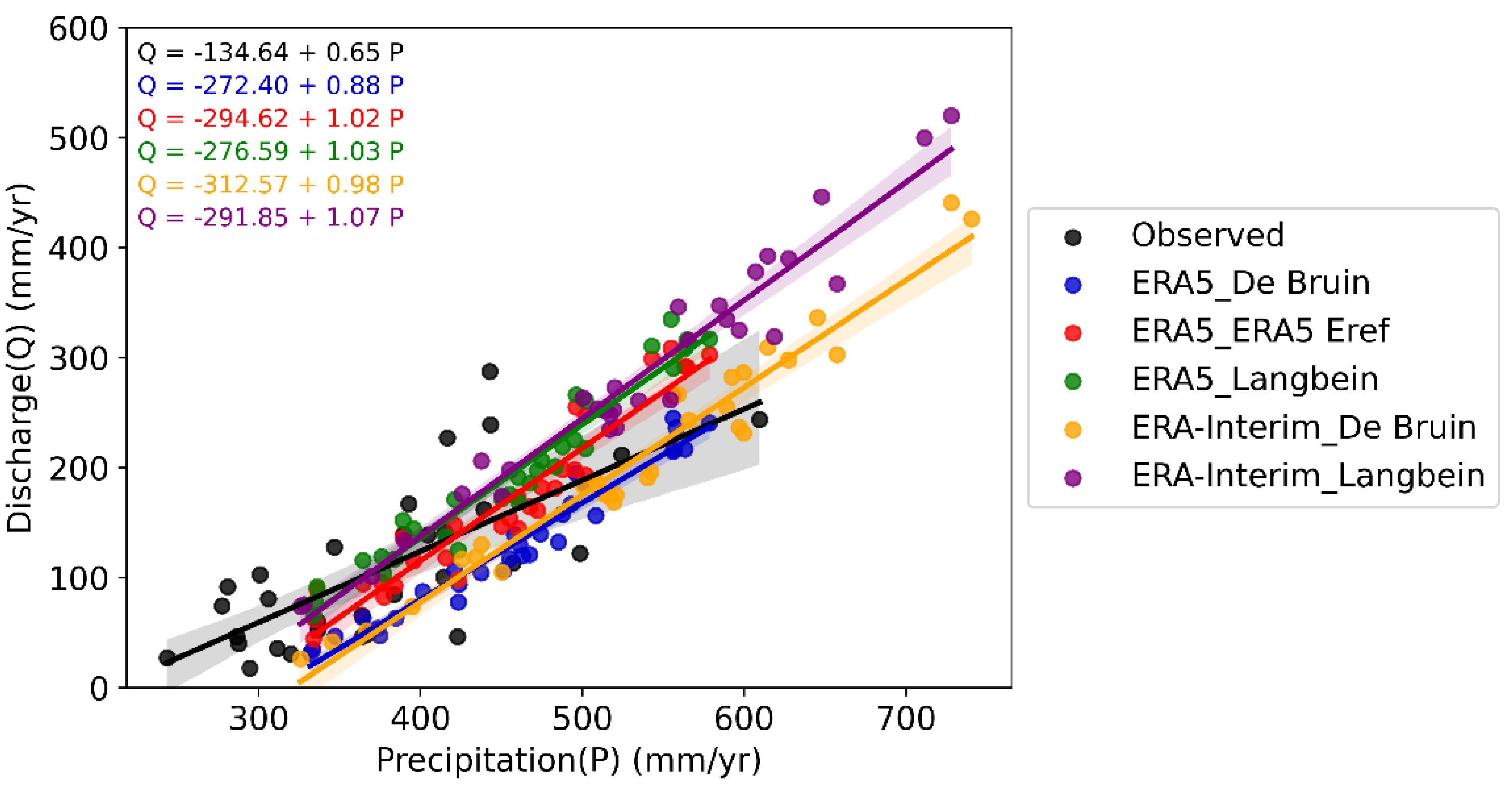
From 2006 to 2016, the model did not perform as well as it did from 1986 to 2006. This could be due to the model’s sensitivity to precipitation, as the differences between the precipitation datasets and the observed precipitation were larger from 2006 to 2016 than from 1986 to 2006. Therefore, we plotted the discharge versus precipitation to determine the model’s sensitivity to estimating the discharge from input precipitation. Figure 8 illustrates that the GlobWat model is extremely sensitive to precipitation. Generally, a 10% increase in precipitation results in a 38% increase in discharge.
Human interventions may have contributed to the low observed discharge and thus the poor model performance between 2006 and 2016. Human interventions have generally increased since 2006. The regulated water volume of water projects in the Urmia Lake Basin, for example, was 1712 MCM in 2006 [70], increasing by 70% (1147.36 MCM) between 2005 and 2009 [71]. Irrigated areas increased 69% (87,919 km2) from 2006 to 2016 (from 114,471 km2 in 2006 to 193,390 km2 in 2016) [72]. Additionally, from 2006 to 2016, the Urmia lake basin provided a yearly average of 206.6 MCM of water for drinking and industrial purposes [73]. Water transfer projects in the basin also reduced the amount of observed discharge in the basin. For example, there was a large transfer of 157 MCM per year of potable water from Zarrineh Rood to Tabriz City in the Urmia Lake Basin in 1999 [67]. Table S4 in the Supplementary Materials provides an overview of the basin’s water and irrigation projects.
The Urmia Lake Basin is endorheic. Thus, human interventions in the basin affect the water volume stored in Urmia Lake. One of the human interventions in the basin was the expansion of irrigated areas. As a result, we depicted the changes in the Urmia Lake area and irrigated areas between 1986 and 2016. In this way, we can see when human interferences occurred at a faster rate. Figure 9 shows the lake gradually shrinking from 1986 to 2006, followed by rapid shrinking from 2006 to 2016. In comparison, the irrigated land area increased more slowly from 1986 to 2006 and more rapidly from 2006 to 2016. In general, increasing the amount of irrigated land correlates with a decrease in the lake area.
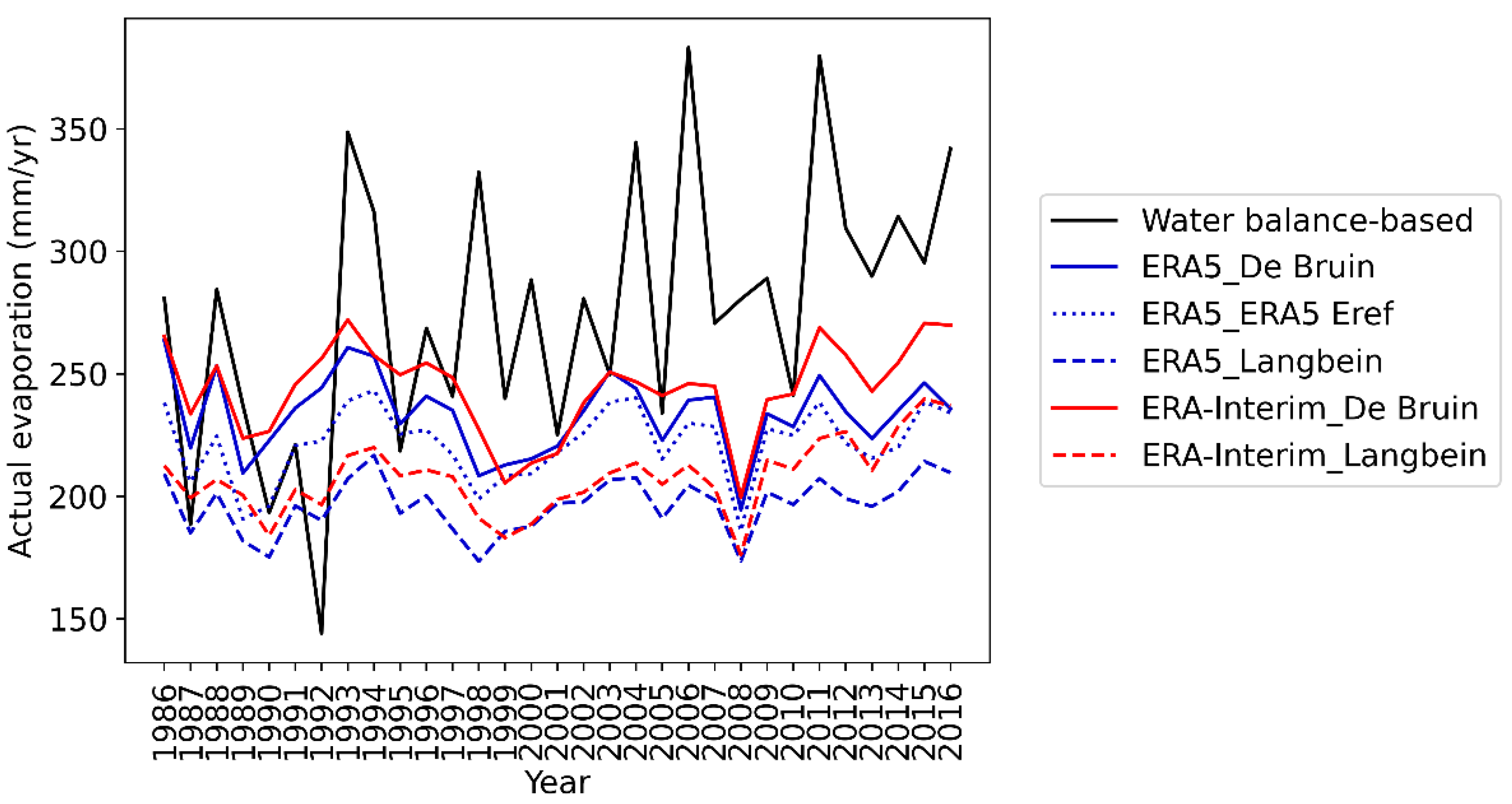
GlobWat estimates Eact by multiplying Eref by a crop or land use factor, which is assumed to be equal to the maximum evaporation of a land use or vegetation type [16]. We analyzed the Eact results for the Urmia Lake Basin, which were calculated by GlobWat for each basin around the world. Eact was estimated using the observed data and a water balance equation (Equation (1)) because it could not be measured directly in the Urmia Lake Basin [62]. Figure 10 shows the Eact for the Urmia Lake Basin, as estimated by GlobWat and based on the observed data. In all experiments, GlobWat underestimated Eact.
Table 2 shows the CC and RMSE between the estimated and calculated Eact. GlobWat Eact estimates had a low correlation with the observed Eact calculated using the water balance equation (Equation (1)). When the De Bruin method was used to calculate Eact, the lowest RMSEs were obtained for all periods. D. Moshir Panahi et al. [62] estimated the mean Eact to be 275 (mm/yr) from 1986 to 2016, which is close to the mean Eact value estimated by GlobWat using a combination of the De Bruin_ERA-Interim (244 mm/yr) and De Bruin_ERA5 (234 mm/yr). In general, GlobWat performed better when using the De Bruin method and ERA-Interim in estimating the Eact. We should consider that D. Moshir Panahi et al. [62] calculated Eact using a water balance equation. This means that all the errors accumulated in the estimate of Eact, which can partially explain the large variation in the Eact calculated by D. Moshir Panahi et al. [62].

4. Discussion

4.1. Development of Scripts for Processing Weather Input Data for GlobWat

The need to automate the complex and time-consuming process of converting climate datasets into GlobWat input motivated the development of ESMValTool Python and YAML scripts for processing ERA5 and ERA-Interim data to the GlobWat input data format. An important aspect of this study is that the scripts, reviewed by the ESMValTool software development community, ensure that they are based on the best code practices. In addition to the technical review of the scripts, before publishing the scripts in the ESMValTool repository, ESMValTool scientific reviewers checked the science behind the scripts to ensure correct inputs are created for the use in the GlobWat model. The history of script development and reviews can be found in the ESMValTool pull requests [74]. As the scripts are published in the ESMValTool repository, there is the opportunity to obtain guidance from the developers of the ESMValTool community as well as future maintenance of the scripts. The first goal of this article is to introduce the scientific community to these scripts.
The scripts reduce the amount of time and effort required to prepare input data for the GlobWat model and ensure the creation of proper weather input data. Hydrologists can now allocate less time to data extraction and formatting. As a result, they can move from concept to experimentation with GlobWat much more quickly. Python and YAML scripting-based data processing improve the GlobWat model’s reproducibility and repeatability, as the same script can be reused. When used in a new study, the scripts only need a few user inputs (e.g., the study period, Eref method, study period, and dataset). The provenance of the data processing steps is recorded by the Python and YAML scripts. For example, the provenance stores information about which raw input files were used to create which files. This ensures reproducibility because researchers will be able to repeat the experiment and obtain the same results [75]. Another important aspect of this study is that the development of the Python and YAML input data processing approaches can be transferred to other GHMs when writing scripts for other grid-based GHMs.

4.2. Comparison of ERA5 and ERA-Interim Precipitation and Temperature with Observed Data in Urmia Lake Basin

In comparison to ERA-Interim, ERA5 provided a better representation of precipitation in the Urmia Lake Basin. Our findings are consistent with previous studies that showed that ERA5 precipitation correlates better with observed data than ERA-Interim [76,77,78]. ERA5 has several improvements over ERA-Interim, including higher spatial resolution, a larger number of observation datasets for the assimilation system, and the inclusion of satellite precipitation estimates [79]. These improvements could explain why ERA5 performs better in precipitation representation. When ERA5 and ERA-Interim temperatures were compared to the observed temperatures in the Urmia Lake Basin, ERA5 did not outperform ERA-Interim. Our findings are in agreement with those of A. Delhasse et al. [80] and L. Liu et al. [81].
Previous studies compared the accuracy of ERA5 to observed data from several basins in Iran, indicating that ERA5 can be used as a potential source of weather data in basins with low densities of meteorological stations [82,83]. We also recommend using ERA5 as a source of weather data in the Urmia Lake Basin, which is consistent with the findings of M. Habibi et al. [84].

4.3. GlobWat Discharge and Eact Estimates for the Urmia Lake Basin

As weather input data, GlobWat requires precipitation and Eref. We used ERA5 and ERA-Interim precipitation. We calculated the reference evaporation using the ERA5 and ERA-interim meteorological variables using two Eref methods, De Bruin and Langbein. The De Bruin method is radiation-based, whereas the Langbein method is an empirical temperature-based method. Given the cold and semi-arid climate of the Urmia Lake Basin, De Bruin estimated a higher Eref for the Urmia Lake Basin in comparison to Langbein.
Our results show that the model performed best in estimating the discharge when the ERA5 dataset and the De Bruin Eref method were used as model inputs. One reason is that GlobWat’s discharge is highly sensitive to precipitation. ERA5 has significantly better precipitation than ERA-Interim. According to some studies, the choice of Eref in hydrological modeling has little effect on the hydrological modeling and estimated discharge [85,86]. However, in the case of the Urmia Lake Basin, the Eref method had a major impact on the discharge estimates. Part of the reason why discharge based on De Bruin was closer to the observed discharge than discharge based on Langbein is that ERA5 and ERA-Interim over-estimated precipitation, especially from 2006 onwards (see next section). This means that the high Eref values that De Bruin produced may offset the overestimated precipitation.
GlobWat’s discharge estimates did not match the observed discharge pattern from 2006 to 2016. The main reason for this disparity was the low correlation between ERA5 and ERA-Interim precipitation and the observed precipitation during this period. The GlobWat model is highly sensitive to precipitation, and the overestimation of precipitation caused an overestimation of discharge. Another reason for the overestimation could be human intervention in the Urmia Lake Basin. Human interventions in the Urmia Lake Basin increased significantly since 2006, resulting in low discharge to the lake and a smaller lake area. As a global scale model, the GlobWat model is incapable of capturing these changes. For the lack of direct measurements, the actual evaporation was estimated using the water balance equation (water-balance Eact) [62]. The water-balance Eact varies greatly over time because all errors in the other terms accumulate in the estimated evaporation.
Our results showed that ERA5 can be used as an input for hydrological modeling in the Urmia Lake Basin but caution has to be taken with respect to recent precipitation.

5. Practical Implications of This Study

The ESMValTool scripts for processing input data for GlobWat can be used in global hydrological modeling with GlobWat to assess water use in agriculture, renewable water resources, and the amount of blue water (incremental evaporation) and green water (evaporation from in situ rainfall) [16]. The assessments can be global or local. Data manipulation for use in the GlobWat model was simplified with the help of the developed scripts, paving the way for future research. Examples are using the scripts for calculating Eref with other methods or using datasets with higher spatial and temporal resolutions. The assessment of the optimal resolution or Eref methods will be part of future research that will benefit from GlobWat’s automated and repeatable model input creation. The lack of data on model-estimated variables, such as Eact, was one of the study’s challenges.

6. Conclusions

Global hydrological models (GHMs) are increasingly using high-resolution datasets, which makes data processing complex and time-consuming, limiting GHM use to groups with the required programming and technical skills. GlobWat, a high-resolution GHM developed by the FAO to assess water use in agriculture, is one of these high-resolution GHMs. A set of Python and YAML scripts was created within the ESMValTool to convert ECMWF ERA5 and ERA-Interim weather data to the format required by GlobWat. This study develops and demonstrates the ability to support a streamlined, reproducible process for creating input data for the GlobWat GHM. These scripts automate downloading and standardizing raw data, calculating reference evaporation, unit conversion, and re-gridding to provide data input for GlobWat. Although these scripts are intended to create GlobWat input requirements from ERA5 and ERA-Interim, they could be adapted to process other datasets for use in GlobWat or to create input data for other grid-based GHMs that use a similar input data format. The usefulness of the scripts was demonstrated through the application of 30 years of processed ERA5 and ERA-Interim data in GlobWat. As an example case study, the results of GlobWat were evaluated for the Urmia Lake Basin in Iran. Based on our overall evaluation and the results from the Urmia Lake Basin, the major findings are as follows:
  • Using developed scripts within the ESMValTool allowed the rapid analysis of the underlying causes of observed trends.
  • The provenance made reproducibility easier by storing information from previous analyses. For example, in our study, we were able to look back and see which raw input files were used to create which files and so on.
  • When compared to its previous version, ERA-Interim, the ERA5 representation of temperature has not improved significantly over the Urmia Lake Basin. However, the ERA5 precipitation representation has significantly improved over the Urmia Lake basin.
  • In basins with low densities of meteorological stations, such as the Urmia Lake Basin, ERA5 can be a good source of weather data.
  • In the Urmia Lake basin, the De Bruin radiation Eref method outperformed the Langbein temperature-based method when evaluated in terms of the modeled and measured discharge.
  • The GlobWat discharge estimates are extremely sensitive to precipitation in (semi-) arid regions. Therefore, ERA5 would be preferable over ERA-Interim due to the better representation of precipitation.
  • The GlobWat model does not capture human interactions in the basin.
In this light, we have demonstrated that, when using the provided framework, rapid and reproducible comparisons can be made. On the ESMValTool website [49,50], all curated code is freely available for use by interested researchers. Any researcher should be able to replicate the findings and conduct new research.

Supplementary Materials

The following supporting information can be downloaded at: https://www.mdpi.com/article/10.3390/w14121950/s1, Table S1: The comparison of evaluation statistics for ERA5 and ERA-Interim precipitation in three time periods; Table S2: The comparison of evaluation statistics for ERA5 and ERA-Interim temperature in three time periods; Table S3: Calculated statistics between GlobWat estimated and observed discharge in three time periods; Table S4: Major Dams of Urmia Lake Basin.

Author Contributions

Conceptualization, B.A. and N.v.d.G.; methodology, B.A. and F.A.; software, B.A. and F.A.; validation, B.A. and D.M.P.; formal analysis, B.A.; investigation, B.A., F.A. and N.v.d.G.; resources, B.A., R.H. and N.v.d.G.; data curation, B.A., F.A. and D.M.P.; writing—original draft preparation, B.A.; writing—review and editing, B.A., F.A. and N.v.d.G.; visualization, B.A.; supervision, F.A. and N.v.d.G.; project administration, B.A.; funding acquisition, B.A., R.H. and N.v.d.G. All authors have read and agreed to the published version of the manuscript.

Funding

We acknowledge funding support from The Netherlands eScience Center through project number 027.017.F01 ‘eWatercycle II’.

Institutional Review Board Statement

It is not relevant to the study.

Informed Consent Statement

It is not relevant to the study.

Data Availability Statement

GlobWat data processing scripts, details on how to access the sample data, the GlobWat model, and ERA5 and ERA-Interim datasets are available on the ESMValTool documentation and GitHub page: https://docs.esmvaltool.org/en/latest/recipes/recipe_hydrology.html?highlight=hydrology (accessed on 17 June 2022) and https://github.com/ESMValGroup/ESMValTool/tree/main/esmvaltool (accessed on 17 June 2022). Please cite the GlobWat recipe and diagnostic using the citation information available at https://doi.org/10.5281/zenodo.3974591 (accessed on 17 June 2022).

Acknowledgments

We thank the Netherlands eScience Center’s team working on the eWaterCycle II project for their support. We would also like to thank Peter Kalverla and Jerom Aerts for their technical and scientific review of the GlobWat processing scripts.

Conflicts of Interest

There is no conflict of interest.

Appendix A

Table A1. GlobWat input layers and their sources.
Input LayerSource
Global maps of monthly precipitationERA5 and ERA-Interim reanalysis products from ECMWF [28,57]
Global maps of wet days per monthProvided by model developers from New et al. [30]
Global maps of coefficient of variation of precipitation per monthProvided by model developers from New et al. [30]
Global maps of monthly reference evaporationCalculated according to Langbein and De Bruin methods with input data from ERA5 and ERA-Interim reanalysis products from ECMWF [28,57]
Maximum soil moisture storage capacityProvided by model developers from the Harmonised World Soil Database, FAO [34]
Maximum groundwater recharge fluxProvided by model developers from WHYMAP, BGR, and UNESCO [33]
Land use or vegetation type coefficientProvided by model developers from FAO’s Global Agricultural Systems Map, FAO [32]
Global map of irrigation areasProvided by model developers from Siebert et al. [35]
Global map of lakes and wetlandsProvided by model developers from Lehner and Döll [31]
Global map of river basins and sub-basinsProvided by model developers from FAO [32]

Appendix B

Steps for running the GlobWat model with ERA5 and ERA-Interim data as inputs using processing scripts developed in this study.
The GlobWat model’s instructions, input data, model code, and ERA5/ERA-Interim data processor scripts (GlobWat recipe and diagnostic) are all freely available online. To run the GlobWat model using the recipe and diagnostic developed in this study, follow the steps below. All relevant links are provided.
  • Download the GlobWat model and its input data from the FAO’s AquaMaps website [17].
  • Follow the instructions on the ESMValTool Website [87] to install the ESMValTool on your system.
  • Using the reference method, select the variables needed for processing data for use in the GlobWat model. More information can be found in the ESMValTool Documentation [88].
  • Using download_era_interim.py [51], download the variables you require from ERA-Interim for the time period you require.
  • Using era5cli [52], download the variables you need for the desired time period.
  • Use CMORizers [53] to CMORize ERA-Interim and ERA5. More information on using a CMORizer can be found at using-a-cmorizer-script [89].
  • At recipe recipe_globwat.yml [49], select the time period and reference method with which you would like to process the data.
  • Use the Running [90] command to execute the recipe_globwat.yml [49].
  • Save the newly processed precipitation and reference evaporation to the GlobWat model input folder.
  • Run the GlobWat model as described in How_to_use_GlobWatv1.0rev2.pdf [36].
  • Using any CSV or ASCII reader, extract the results for your desired location.

References

  1. Essawy, B.T.; Goodall, J.L.; Xu, H.; Gil, Y. Evaluation of the OntoSoft Ontology for describing metadata for legacy hydrologic modeling software. Environ. Model. Softw. 2017, 92, 317–329. [Google Scholar] [CrossRef] [Green Version]
  2. Hutton, C.; Wagener, T.; Freer, J.; Han, D.; Duffy, C.; Arheimer, B. Most computational hydrology is not reproducible, so is it really science? Water Resour. Res. 2016, 52, 7548–7555. [Google Scholar] [CrossRef]
  3. Rosenberg, D.E.; Filion, Y.; Teasley, R.; Sandoval-Solis, S.; Hecht, J.S.; van Zyl, J.E.; McMahon, G.F.; Horsburgh, J.S.; Kasprzyk, J.R.; Tarboton, D.G. The Next Frontier: Making Research More Reproducible. J. Water Resour. Plan. Manag. 2020, 146, 01820002. [Google Scholar] [CrossRef] [Green Version]
  4. Hut, R.; Drost, N.; Aerts, J.; Bouaziz, L.; van Verseveld, W.; Jagers, B.; Sutanudjaja, E.; Melsen, L.; Bennett, A.; Arnal, L.; et al. Comparing the Impact for Hydrology of the New ERA5 Reanalyses Dataset over ERA-Interim for 8 Hydrological Models in 6 Catchments Using the EWaterCycle Community Modelling Environment. In Proceedings of the EGU General Assembly, Online, 4–8 May 2020. [Google Scholar]
  5. Hut, R.; Drost, N.; van de Giesen, N.; van Werkhoven, B.; Abdollahi, B.; Aerts, J.; Albers, T.; Alidoost, F.S.; Andela, B.; Camphuijsen, J.; et al. The EWaterCycle Platform for Open and FAIR Hydrological Collaboration. Geosci. Model Dev. 2021. [Google Scholar] [CrossRef]
  6. Hall, C.A.; Saia, S.M.; Popp, A.L.; Dogulu, N.; Schymanski, S.J.; Drost, N.; van Emmerik, T.; Hut, R. A hydrologist’s guide to open science. Hydrol. Earth Syst. Sci. 2021, 26, 647–664. [Google Scholar] [CrossRef]
  7. Essawy, B.T.; Goodall, J.L.; Voce, D.; Morsy, M.M.; Sadler, J.M.; Choi, Y.D.; Tarboton, D.G.; Malik, T. A taxonomy for reproducible and replicable research in environmental modelling. Environ. Model. Softw. 2020, 134, 104753. [Google Scholar] [CrossRef]
  8. Stagge, J.H.; Rosenberg, D.E.; Abdallah, A.M.; Akbar, H.; Attallah, N.A.; James, R. Assessing data availability and research reproducibility in hydrology and water resources. Sci. Data 2019, 6, 190030. [Google Scholar] [CrossRef] [Green Version]
  9. Janssen, M.A.; Pritchard, C.; Lee, A. On code sharing and model documentation of published individual and agent-based models. Environ. Model. Softw. 2020, 134, 104873. [Google Scholar] [CrossRef]
  10. Piccolo, S.R.; Frampton, M.B. Tools and techniques for computational reproducibility. GigaScience 2016, 5, 30. [Google Scholar] [CrossRef] [Green Version]
  11. Siderius, C.; Biemans, H.; Kashaigili, J.J.; Conway, D. Going local: Evaluating and regionalizing a global hydrological model’s simulation of river flows in a medium-sized East African basin. J. Hydrol. Reg. Stud. 2018, 19, 349–364. [Google Scholar] [CrossRef]
  12. Bierkens, M.F.P.; Bell, V.A.; Burek, P.; Chaney, N.; Condon, L.E.; David, C.H.; de Roo, A.; Döll, P.; Drost, N.; Famiglietti, J.S.; et al. Hyper-resolution global hydrological modelling: What is next?: “Everywhere and Locally Relevant”. Hydrol. Process. 2015, 29, 310–320. [Google Scholar] [CrossRef]
  13. Wilkinson, M.D.; Dumontier, M.; Aalbersberg, I.J.; Appleton, G.; Axton, M.; Baak, A.; Blomberg, N.; Boiten, J.W.; da Silva Santos, L.B.; Bourne, P.E.; et al. The FAIR Guiding Principles for scientific data management and stewardship. Sci. Data 2016, 3, 160018. [Google Scholar] [CrossRef] [PubMed] [Green Version]
  14. Horsburgh, J.S.; Morsy, M.M.; Castronova, A.M.; Goodall, J.L.; Gan, T.; Yi, H.; Stealey, M.J.; Tarboton, D.G. HydroShare: Sharing Diverse Environmental Data Types and Models as Social Objects with Application to the Hydrology Domain. JAWRA J. Am. Water Resour. Assoc. 2015, 52, 873–889. [Google Scholar] [CrossRef] [Green Version]
  15. Gichamo, T.Z.; Sazib, N.S.; Tarboton, D.G.; Dash, P. HydroDS: Data services in support of physically based, distributed hydrological models. Environ. Model. Softw. 2020, 125, 104623. [Google Scholar] [CrossRef]
  16. Hoogeveen, J.; Faurès, J.-M.; Peiser, L.; Burke, J.; van de Giesen, N. GlobWat—A global water balance model to assess water use in irrigated agriculture. Hydrol. Earth Syst. Sci. 2015, 19, 3829–3844. [Google Scholar] [CrossRef] [Green Version]
  17. AQUASTAT (FAO). Available online: https://data.apps.fao.org/catalog//iso/c26de669-90f9-43a1-ae4d-6b1b9660f5e0 (accessed on 7 May 2022).
  18. Eyring, V.; Bock, L.; Lauer, A.; Righi, M.; Schlund, M.; Andela, B.; Arnone, E.; Bellprat, O.; Brötz, B.; Caron, L.-P.; et al. Earth System Model Evaluation Tool (ESMValTool) v2.0—An extended set of large-scale diagnostics for quasi-operational and comprehensive evaluation of Earth system models in CMIP. Geosci. Model Dev. 2020, 13, 3383–3438. [Google Scholar] [CrossRef]
  19. Obtaining Input Data for ESMValTool 2.5.0. Available online: https://docs.esmvaltool.org/en/latest/input.html?highlight=cruera5#supported-datasets-for-which-a-cmorizer-script-is-available (accessed on 3 June 2022).
  20. Pokhrel, Y.N.; Hanasaki, N.; Wada, Y.; Kim, H. Recent progresses in incorporating human land–water management into global land surface models toward their integration into Earth system models. WIREs Water 2016, 3, 548–574. [Google Scholar] [CrossRef] [Green Version]
  21. Bierkens, M.F.P. Global hydrology 2015: State, trends, and directions. Water Resour. Res. 2015, 51, 4923–4947. [Google Scholar] [CrossRef]
  22. Tarek, M.; Brissette, F.P.; Arsenault, R. Evaluation of the ERA5 reanalysis as a potential reference dataset for hydrological modelling over North America. Hydrol. Earth Syst. Sci. 2020, 24, 2527–2544. [Google Scholar] [CrossRef]
  23. Chaudhuri, A.H.; Ponte, R.M.; Forget, G.; Heimbach, P. A Comparison of Atmospheric Reanalysis Surface Products over the Ocean and Implications for Uncertainties in Air–Sea Boundary Forcing. J. Clim. 2013, 26, 153–170. [Google Scholar] [CrossRef]
  24. Dee, D.; Fasullo, J.; Shea, D.; Walsh, J. National Center for Atmospheric Research Staffs(Eds) Page. Available online: https://climatedataguide.ucar.edu/climate-data/atmospheric-reanalysis-overview-comparison-tables (accessed on 5 May 2022).
  25. Matveeva, T.; Sidorchuk, A. Modelling of Surface Runoff on the Yamal Peninsula, Russia, Using ERA5 Reanalysis. Water 2020, 12, 2099. [Google Scholar] [CrossRef]
  26. Eisner, S. Comprehensive Evaluation of the WaterGAP3 Model across Climatic, Physiographic, and Anthropogenic Gradients. Ph.D. Thesis, University of Kassel, Kassel, Germanny, 8 December 2015. [Google Scholar]
  27. Schaphoff, S.; Forkel, M.; Müller, C.; Knauer, J.; von Bloh, W.; Gerten, D.; Jägermeyr, J.; Lucht, W.; Rammig, A.; Thonicke, K.; et al. LPJmL4—A dynamic global vegetation model with managed land—Part 2: Model evaluation. Geosci. Model Dev. 2018, 11, 1377–1403. [Google Scholar] [CrossRef]
  28. Hersbach, H.; Bell, B.; Berrisford, P.; Hirahara, S.; Horanyi, A.; Muñoz-Sabater, J.; Nicolas, J.; Peubey, C.; Radu, R.; Schepers, D.; et al. The ERA5 global reanalysis. Q. J. R. Meteorol. Soc. 2020, 146, 1999–2049. [Google Scholar] [CrossRef]
  29. Hoffmann, L.; Günther, G.; Li, D.; Stein, O.; Wu, X.; Griessbach, S.; Heng, Y.; Konopka, P.; Müller, R.; Vogel, B.; et al. From ERA-Interim to ERA5: The considerable impact of ECMWF’s next-generation reanalysis on Lagrangian transport simulations. Atmos. Chem. Phys. 2019, 19, 3097–3124. [Google Scholar] [CrossRef] [Green Version]
  30. New, M.; Lister, D.; Hulme, M.; Makin, I. A high-resolution data set of surface climate over global land areas. Clim. Res. 2002, 21, 1–25. [Google Scholar] [CrossRef] [Green Version]
  31. Lehner, B.; Döll, P. Development and validation of a global database of lakes, reservoirs and wetlands. J. Hydrol. 2004, 296, 1–22. [Google Scholar] [CrossRef]
  32. FAO. The State of the World’s Land and Water Resources for Food and Agriculture (SOLAW)—Managing Systems at Risk; Food and Agriculture Organization of the United Nations/Earthscan: Rome, Italy; London, UK, 2011; pp. 1–285. [Google Scholar]
  33. The Official United Nations Site for The Millennium Development Goals Indicators. Available online: https://mdgs.un.org/unsd/mdg/Host.aspx?Content=indicators/officiallist.htm (accessed on 4 May 2022).
  34. FAO. FAO Water Reports 38 Coping with Water Scarcity: An Action Framework for Agriculture and Food Security; Food and Agri-culture Organization of the United Nations: Rome, Italy, 2012. [Google Scholar]
  35. Siebert, S.; Döll, P.; Feick, S.; Hoogeveen, J.; Frenken, K. Global Map of Irrigation Areas v5.0 (GIMA). Available online: https://aquaknow.jrc.ec.europa.eu/en/content/global-map-irrigated-areas-v50-gmia (accessed on 4 May 2022).
  36. How to Use GlobWat 1.0. Available online: https://github.com/Jippe-FAO/GlobWat/blob/master/HowtouseGlob-Wat1-0.pdf (accessed on 4 May 2022).
  37. Righi, M.; Andela, B.; Eyring, V.; Lauer, A.; Predoi, V.; Schlund, M.; Vegas-Regidor, J.; Bock, L.; Brötz, B.; De Mora, L.; et al. Earth System Model Evaluation Tool (ESMValTool) v2.0—Technical overview. Geosci. Model Dev. 2020, 13, 1179–1199. [Google Scholar] [CrossRef] [Green Version]
  38. ECMWF Parameter Details. Available online: https://apps.ecmwf.int/codes/grib/param-db?id=228251 (accessed on 2 May 2022).
  39. De Bruin, H.A.R.; Trigo, I.F.; Bosveld, F.C.; Meirink, J.F. A Thermodynamically Based Model for Actual Evapotranspiration of an Extensive Grass Field Close to FAO Reference, Suitable for Remote Sensing Application. J. Hydrometeorol. 2016, 17, 1373–1382. [Google Scholar] [CrossRef]
  40. Andela, B.; Broetz, B.; de Mora, L.; Drost, N.; Eyring, V.; Koldunov, N.; Lauer, A.; Mueller, B.; Predoi, V.; Righi, M.; et al. ESMValTool (v2.5.0). Zenodo 2022, 1–43. Available online: https://doi.org/10.5281/ZENODO.6359405 (accessed on 17 June 2022). [CrossRef]
  41. Verhoeven, S.; Drost, N.; Weel, B.; Smeets, S.; Kalverla, P.; Alidoost, F.; Vreede, B.; Hut, R.; Aerts, J.; van Werkhoven, B.; et al. EWaterCycle Python Package (1.3.0). Zenodo 2022. Available online: https://doi.org/10.5281/ZENODO.6472252 (accessed on 17 June 2022). [CrossRef]
  42. Langbein, W.B. Geological Survey Circular 52 Annual Runoff in the United States; USGS: Washington, DC, USA, 1949. [Google Scholar] [CrossRef]
  43. Stockton, C.W.; Boggess, W.R. Geohydrological Implications of Climate Change on Water Resource Development; Laboratory of Tree-Ring Research, University of Arizona: Tucson, AZ, USA, 1979. [Google Scholar]
  44. Shibuo, Y.; Jarsjö, J.; Destouni, G. Hydrological responses to climate change and irrigation in the Aral Sea drainage basin. Geophys. Res. Lett. 2007, 34, L21406. [Google Scholar] [CrossRef]
  45. Shi, H.; Li, T.; Wang, G. Temporal and spatial variations of potential evaporation and the driving mechanism over Tibet during 1961–2001. Hydrol. Sci. J. 2017, 62, 1469–1482. [Google Scholar] [CrossRef] [Green Version]
  46. Jarsjö, J.; Törnqvist, R.; Su, Y. Climate-driven change of nitrogen retention–attenuation near irrigated fields: Multimodel projections for Central Asia. Environ. Earth Sci. 2017, 76, 117. [Google Scholar] [CrossRef] [Green Version]
  47. Asokan, S.M.; Jarsjö, J.; Destouni, G. Vapor flux by evapotranspiration: Effects of changes in climate, land use, and water use. J. Geophys. Res. 2010, 115, D24102. [Google Scholar] [CrossRef] [Green Version]
  48. Jaramillo, F.; Prieto, C.; Lyon, S.W.; Destouni, G. Multimethod assessment of evapotranspiration shifts due to non-irrigated agricultural development in Sweden. J. Hydrol. 2013, 484, 55–62. [Google Scholar] [CrossRef] [Green Version]
  49. ESMValTool GlobWat Recipe. Available online: https://github.com/ESMValGroup/ESMValTool/blob/main/esmvaltool/recipes/hydrology/recipe_globwat.yml (accessed on 9 May 2022).
  50. ESMValTool GlobWat Diagnostic. Available online: https://github.com/ESMValGroup/ESMValTool/blob/main/esmvaltool/diag_scripts/hydrology/globwat.py (accessed on 9 May 2022).
  51. ESMValTool Download ERA-Interim. Available online: https://github.com/ESMValGroup/ESMValTool/blob/main/esmvaltool/cmorizers/data/download_scripts/download_era_interim.py (accessed on 2 May 2022).
  52. Era5cli 1.0.0 Documentation. Available online: https://era5cli.readthedocs.io/en/stable/ (accessed on 2 May 2022).
  53. ESMValTool GitHub ERA-Interim Cmorizer. Available online: https://github.com/ESMValGroup/ESMValTool/blob/a9b6592a02f2085634a214ff5f36a736fa18ff47/esmvaltool/cmorizers/obs/cmorize_obs_era_interim.py (accessed on 2 May 2022).
  54. ESMValTool GitHub ERA5 Cmorizer. Available online: https://github.com/ESMValGroup/ESMValTool/blob/main/esmvaltool/recipes/cmorizers/recipe_daily_era5.yml (accessed on 7 May 2022).
  55. ECMWF Reference Guide. Available online: https://confluence.ecmwf.int/display/EMOS/Precipitation (accessed on 2 May 2022).
  56. ESMValTool 2.5.0 Documentation. Available online: https://docs.esmvaltool.org/en/latest/recipes/recipe_hydrology.html?highlight=hydrology (accessed on 2 May 2022).
  57. Dee, D.P.; Uppala, S.M.; Simmons, A.J.; Berrisford, P.; Poli, P.; Kobayashi, S.; Andrae, U.; Balmaseda, M.A.; Balsamo, G.; Bauer, P.; et al. The ERA-Interim reanalysis: Configuration and performance of the data assimilation system. Q. J. R. Meteorol. Soc. 2011, 137, 553–597. [Google Scholar] [CrossRef]
  58. Berrisford, P.; Dee, D.; Fielding, K.; Fuentes, M.; Kallberg, P.; Kobayashi, S.; Uppala, S.; Simmons, A. ERA Report Series 1 The ERA-Interim Archive; European Centre for Medium Range Weather Forecasts: Berkshire, UK, 2009; Available online: https://www.ecmwf.int/file/21497/download?token=j_b81H0z (accessed on 17 June 2022).
  59. ECMWF Datasets (ERA5). Available online: https://www.ecmwf.int/en/forecasts/datasets/reanalysis-datasets/era5 (accessed on 2 May 2022).
  60. ECMWF Datasets (ERA-Interim). Available online: https://www.ecmwf.int/en/forecasts/datasets/reanalysis-datasets/era-interim (accessed on 2 May 2022).
  61. Essou, G.R.C.; Brissette, F.; Lucas-Picher, P. The Use of Reanalyses and Gridded Observations as Weather Input Data for a Hydrological Model: Comparison of Performances of Simulated River Flows Based on the Density of Weather Stations. J. Hydrometeorol. 2017, 18, 497–513. [Google Scholar] [CrossRef]
  62. Moshir Panahi, D.; Kalantari, Z.; Ghajarnia, N.; Seifollahi-Aghmiuni, S.; Destouni, G. Variability and change in the hydro-climate and water resources of Iran over a recent 30-year period. Sci. Rep. 2020, 10, 7450. [Google Scholar] [CrossRef]
  63. Asem, A.; Eimanifar, A.; Wink, M. Update of “Biodiversity of the Hypersaline Urmia Lake National Park (NW Iran)”. Diversity 2016, 8, 6. [Google Scholar] [CrossRef] [Green Version]
  64. Schaaf, T.; Rodrigues, D.C. Managing MIDAs: Harmonising the management of Multi-Internationally Designated Areas: Ramsar sites, World Heritage sites, Biosphere Reserves and UNESCO Global Geoparks; IUCN: Gland, Switzerland, 2016. [Google Scholar] [CrossRef]
  65. Karimi, P.; Pareeth, S.; Michailovsky, C. Rapid Assessment of the Water Accounts in Lake Urmia Basin, Iran (WA-Urmia); IHE: Delft, The Netherland, 2019. [Google Scholar]
  66. Bakhshianlamouki, E.; Masia, S.; Karimi, P.; van der Zaag, P.; Sušnik, J. A system dynamics model to quantify the impacts of restoration measures on the water-energy-food nexus in the Urmia lake Basin, Iran. Sci. Total Environ. 2020, 708, 134874. [Google Scholar] [CrossRef]
  67. Alizadeh-Choobari, O.; Ahmadi-Givi, F.; Mirzaei, N.; Owlad, E. Climate change and anthropogenic impacts on the rapid shrinkage of Lake Urmia. Int. J. Clim. 2016, 36, 4276–4286. [Google Scholar] [CrossRef]
  68. Javadzadeh, H.; Ataie-Ashtiani, B.; Hosseini, S.M.; Simmons, C.T. Interaction of lake-groundwater levels using cross-correlation analysis: A case study of Lake Urmia Basin, Iran. Sci. Total Environ. 2020, 729, 138822. [Google Scholar] [CrossRef] [PubMed]
  69. Taylor, K.E. Summarizing multiple aspects of model performance in a single diagram. J. Geophys. Res. Atmos. 2001, 106, 7183–7192. [Google Scholar] [CrossRef]
  70. Hassanzadeh, E.; Zarghami, M.; Hassanzadeh, Y. Determining the Main Factors in Declining the Urmia Lake Level by Using System Dynamics Modeling. Water Resour. Manag. 2012, 26, 129–145. [Google Scholar] [CrossRef]
  71. Hashemi, M. An Independent Review: The Status of Water Resources in the Lake Urmia Basin; Conservation of Iranian Wetlands Project: Tehran, Iran, 2008. [Google Scholar]
  72. Ghale, Y.A.G.; Baykara, M.; Unal, A. Investigating the interaction between agricultural lands and Urmia Lake ecosystem using remote sensing techniques and hydro-climatic data analysis. Agric. Water Manag. 2019, 221, 566–579. [Google Scholar] [CrossRef]
  73. Khatami, S. Nonlinear Chaotic and Trend Analyses of Water Level at Urmia Lake, Iran. Master’s Thesis, Lund University, Lund, Sweden, 2013. [Google Scholar]
  74. Add GlobWat Recipe and Diagnostic by Babdollahi Pull Request #1808. Available online: https://github.com/ESMValGroup/ESMValTool/pull/1808 (accessed on 4 June 2022).
  75. Taylor, K.; Woodcock, R.; Cuddy, S.; Thew, P.; Lemon, D. A Provenance Maturity Model. In Environmental Software Systems. Infrastructures, Services and Applications, 2nd ed.; Denzer, R., Argent, R.M., Schimak, G., Hřebíček, J., Eds.; Springer International Publishing: Cham, Switzerland, 2015; Volume 448, pp. 1–18. [Google Scholar] [CrossRef]
  76. Waseem, S.; Muhammad, I.; Rehan, L.; Shahzada, A.; Muhammad, A.; Ahmad, B.; Azam, M.; Hussain, J. Performance Evaluation and Comparison of Observed and Reanalysis Gridded Precipitation Datasets over Pakistan. Theor. Appl. Climatol. 2022. [Google Scholar] [CrossRef]
  77. Nacar, S.; Kankal, M.; Okkan, U. Evaluation of the suitability of NCEP/NCAR, ERA-Interim and, ERA5 reanalysis data sets for statistical downscaling in the Eastern Black Sea Basin, Turkey. Meteorol. Atmos. Phys. 2022, 134, 39. [Google Scholar] [CrossRef]
  78. McElhinny, M.; Beckers, J.F.; Hanes, C.; Flannigan, M.; Jain, P. A high-resolution reanalysis of global fire weather from 1979 to 2018—Overwintering the Drought Code. Earth Syst. Sci. Data 2020, 12, 1823–1833. [Google Scholar] [CrossRef]
  79. Gleixner, S.; Demissie, T.; Diro, G.T. Did ERA5 Improve Temperature and Precipitation Reanalysis over East Africa? Atmosphere 2020, 11, 996. [Google Scholar] [CrossRef]
  80. Delhasse, A.; Kittel, C.; Amory, C.; Hofer, S.; van As, D.; Fausto, R.S.; Fettweis, X. Brief communication: Evaluation of the near-surface climate in ERA5 over the Greenland Ice Sheet. Cryosphere 2020, 14, 957–965. [Google Scholar] [CrossRef] [Green Version]
  81. Liu, L.; Gu, H.; Xie, J.; Xu, Y. How well do the ERA-Interim, ERA -5, GLDAS -2.1 and NCEP-R2 reanalysis datasets represent daily air temperature over the Tibetan Plateau? Int. J. Clim. 2021, 41, 1484–1505. [Google Scholar] [CrossRef]
  82. Yazdandoost, F.; Moradian, S.; Zakipour, M.; Izadi, A.; Bavandpour, M. Improving the precipitation forecasts of the North-American multi model ensemble (NMME) over Sistan basin. J. Hydrol. 2020, 590, 125263. [Google Scholar] [CrossRef]
  83. Fallah, A.; Rakhshandehroo, G.R.; Berg, P.; Sungmin, O.; Orth, R. Evaluation of precipitation datasets against local observations in southwestern Iran. Int. J. Clim. 2020, 40, 4102–4116. [Google Scholar] [CrossRef] [Green Version]
  84. Habibi, M.; Babaeian, I.; Schöner, W. Changing Causes of Drought in the Urmia Lake Basin—Increasing Influence of Evaporation and Disappearing Snow Cover. Water 2021, 13, 3273. [Google Scholar] [CrossRef]
  85. Xu, C. Issues influencing accuracy of hydrological modeling in a changing environment. Water Sci. Eng. 2021, 14, 167–170. [Google Scholar] [CrossRef]
  86. Jayathilake, D.I.; Smith, T. Identifying the Influence of Systematic Errors in Potential Evapotranspiration on Rainfall–Runoff Models. J. Hydrol. Eng. 2022, 27, 04021047. [Google Scholar] [CrossRef]
  87. ESMValTool 2.5.0 Installation Documentation. Available online: https://docs.esmvaltool.org/en/latest/quickstart/installation.html (accessed on 9 May 2022).
  88. ESMValTool 2.5.0 Documentation—Hydrological Models—Data Pre-Processing. Available online: https://docs.esmvaltool.org/en/latest/recipes/recipe_hydrology.html (accessed on 9 May 2022).
  89. ESMValTool 2.5.0 Documentation—Obtaining Input Data. Available online: https://docs.esmvaltool.org/en/latest/input.html#using-a-cmorizer-script (accessed on 9 May 2022).
  90. ESMValTool 2.5.0 Documentation—Running. Available online: https://docs.esmvaltool.org/projects/ESMValCore/en/latest/quickstart/run.html?highlight=esmvaltool%20run%20#running (accessed on 9 May 2022).
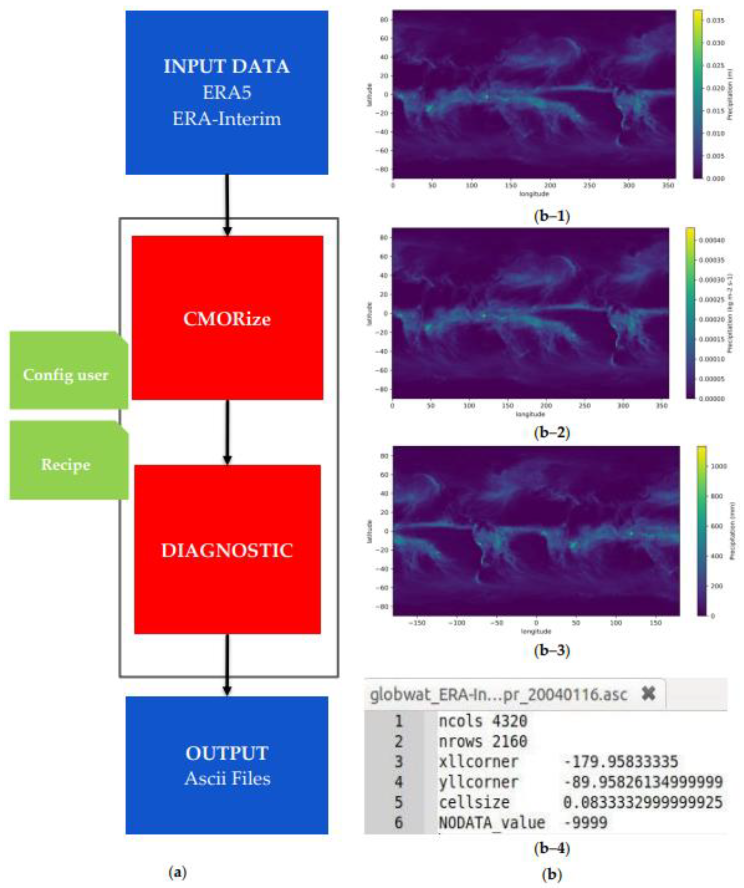
Figure 1. (a) The processing flowchart; (b) Processing example for January precipitation from ERA-Interim dataset; (b–1) Raw data; (b–2) CMORized data; (b–3) Data after application of diagnostic; (b–4) Data in the GlobWat input format.
Water 14 01950 g001
Figure 2. (a) Iran on the world map; (b) Urmia Lake Basin among Iran’s Main Basins; (c) Urmia Lake Basin.
Water 14 01950 g002
Figure 3. (a) Comparison of observed precipitation in the Urmia Lake Basin and ERA5 and ERA-Interim precipitation; (b) Comparison of observed mean annual temperature in the Urmia Lake Basin and ERA5 and ERA-Interim mean annual temperature.
Water 14 01950 g003
Figure 4. Taylor diagram and RMSE comparing ERA5 and ERA-Interim with the observed data in the Urmia Lake Basin during three periods. (a) Mean annual precipitation; (b) Mean annual temperature.
Water 14 01950 g004
Figure 5. Comparison of retrieved reference evaporation (Eref) from ERA5 with Eref values calculated by De Bruin and Langbein methods using ERA5, ERA-Interim, and observed data in the Urmia Lake Basin.
Water 14 01950 g005
Figure 6. Estimated discharge by the GlobWat model using different weather datasets and Eref methods against observed ones over Urmia Lake Basin, Iran.
Water 14 01950 g006
Figure 7. Taylor diagram, RMSE, and NSE comparing the estimated discharge by the GlobWat model using different weather datasets and Eref methods against the observed data in three periods over the Urmia Lake Basin.
Water 14 01950 g007
Figure 8. Scatter plot of precipitation versus discharge for the entire period in the Urmia Lake Basin.
Water 14 01950 g008
Figure 9. Agricultural development and Urmia Lake area changes in the Urmia Lake Basin from 1986 to 2016 [72].
Water 14 01950 g009
Figure 10. Estimated actual evaporation (Eact) calculated by the GlobWat model using different weather datasets and reference evaporation (Eref) methods against the observed data over Urmia Lake, Iran.
Water 14 01950 g010
Table 1. Grid specification (data from GlobWat user manual [36]).
File TypeColumns (X)Rows (Y)Pixel Size (Degree)No Data ValueData TypeReference SystemExtent
AAIGrid: Arc/Info ASCII Grid432021600.08333−9999Float32GCS WGS84−180; −90: 180; 90
Table 2. Comparisons between calculated actual evaporation (Eact) and water balance-based evaporation.
Time PeriodDatasetEref MethodCCRMSE (mm/yr)Mean (mm/yr)
1986–2016Observed 10275
ERA5De Bruin0.367234
ERA5 Eref0.474222
Langbein0.593197
ERA-InterimDe Bruin0.460244
Langbein0.583208
1986–2006Observed 10257
ERA5De Bruin0.355234
ERA5 Eref0.461220
Langbein0.579195
ERA-InterimDe Bruin0.254241
Langbein0.473203
2006–2016Observed 10309
ERA5De Bruin0.485233
ERA5 Eref0.493224
Langbein0.5115200
ERA-InterimDe Bruin0.571249
Langbein0.4100217
Publisher’s Note: MDPI stays neutral with regard to jurisdictional claims in published maps and institutional affiliations.