Abstract
Diel vertical migration of the copepod the community was investigated in the open South Adriatic, in June 2020 and February 2021, under two very different hydrographical conditions. The influence of a winter wind-induced mixing event on copepod vertical migration at the species level was determined for the first time and compared to the situation in June when pronounced thermal stratification was observed. The samples were collected during a 24 h cycle in four depth layers from the surface down to 300 m depth, using a Nansen opening–closing net with 250-µm mesh size. In winter, the bulk of the copepod population remained in the epipelagic zone (0–100 m) over the entire 24 h cycle, with calanoids remaining the dominant group. An increasing trend of copepod standing stocks from midnight to early morning in the surface layer found in June is in agreement with previous records of copepod day–night variations in the Mediterranean Sea. Day–night differences in diversity and the number of taxa of the epipelagic area were more pronounced in June, confirming the higher intensity of diel vertical migration in summer. Although the epipelagic community was composed of numerous weak diel vertical migrant species, for the majority of investigated copepod taxa, migration patterns differed between the environmentally contrasting seasons. A multivariate non-metric analysis showed that the copepod community was strongly affected by temperature, thus exhibiting a clear seasonal structure.
1. Introduction
The vertical distribution of zooplankton depends on a wide range of factors, such as different behaviors (diel, ontogenic and seasonal migrations), local physical features, cyclonic circulation, gyres, etc. [1]. Vertical migration is a widespread behavior of many zooplankton taxa that spans across diel and seasonal timescales. Through vertical migration, organisms actively participate in the transport of matter and energy in the marine environment and play a pivotal role in driving the biological pump. By feeding near the surface and then fasting at a depth where they continue to defecate, respire and excrete, migrating zooplankton remove carbon and nitrogen from the surface layers and release them at depth [2,3].
Diel Vertical Migration (DVM) is the most common behavior and one of the most-studied patterns of animal migration [4,5]. It is mainly of three types. The most common for copepods, as well as other zooplankton groups, involves an ascent to the upper pelagic zone at dusk to feed on phytoplankton during the night and descent to deeper layers at dawn, where the probability of being predated by visual hunting predators is lower. The reverse pattern includes daytime ascent and night-time descent. The third form is a twilight-migration, i.e., a double migration within the 24 h: the ascent occurs during dusk, short presence at the surface, the a descent around midnight, ascent later during the night and descent at dawn [6]. Several biological and physical factors have been proposed to explain the intensity, extent and patterns of DVM. Predatory avoidance is currently considered the ultimate reason for DVM [4,7], although there are contradictory cases, such as species that do not appear to migrate [2] or lack of relationship with predator abundance [8]. Therefore, DVM is generally held to represent a trade-off between the functions of food gathering and avoiding predators [9], which is strongly dependent on environmental variations [10,11,12].
In the marine environment, copepods have successfully colonized the whole marine realm, where their vertical zonation patterns are mainly defined by water depth. Almost the entire Adriatic copepod fauna can be found in the Southern Adriatic (SA), which is characterized by low copepod abundance but high species diversity [13]. Seasonal vertical distribution and DVM patterns of the Adriatic copepods, as well as the other zooplankton groups, have been extensively studied since the middle of the last century [14,15,16,17]. Those investigations mostly included relatively shallow stations above the continental shelf near Dubrovnik [14,15], while for the waters of the open Adriatic, detailed DVM patterns are available for the deep-water copepods during the summer period [16]. Recently, copepod species composition and their vertical and horizontal distribution in the South Adriatic during the winter mixing period were investigated and described in detail [18,19,20]. Additionally, for the first time in the Adriatic Sea, the strength of the backscatter signal from an Acoustic Doppler Current Profiler (ADCP) in relation to zooplankton vertical movement was investigated, including an eleven-year data set [21]. This study described in more detail the poorly known aspects of copepod DVM behavior but not at the species level.
Since the most recent data on copepod diel vertical migration in the SA at the species level is from the middle of the last century, our objective was to elucidate their migration and distribution patterns in light of the new insights into biological and hydroclimatic features of the Adriatic Sea. Short time interval observations were selected to allow a more accurate view of the copepod vertical partitioning under the two contrasting environmental conditions: summer stratification and deep winter convection events. The study investigates to what extent those environmental states influence copepod species-specific seasonal vertical distribution, diversity and diel migratory behavior patterns.
2. Materials and Methods
2.1. Study Area
The Adriatic Sea is a semi-enclosed basin stretching south-eastward for 800 km in the Eastern Mediterranean. The Southern Adriatic (SA) sub-basin represents the deepest part of the Adriatic (up to 1270 m) which interacts with the Eastern Mediterranean through the Strait of Otranto (~800 m depth). This oligotrophic area is a highly complex ecosystem, where vertical mixing (upwelling, wintertime convection) has an important role in homogenizing physical and chemical seawater properties and controlling the primary production [22,23,24]. A major characteristic of the area is a topographically trapped quasi-permanent cyclonic gyre [25,26]. The more saline Levantine Intermediate Water (LIW) is entrained in the gyre, and when exposed to winter episodes of northerly winds, conditions are favorable for deep convection and generation of Adriatic Dense Water (AdDW). The water so formed is then exported through the Strait of Otranto to the rest of the Eastern Mediterranean basin and becomes the main component of the Eastern Mediterranean Deep Water (EMDW) [27]. Water masses, entering the SA in larger amounts during the winter, show a roughly 10-year cycle termed the Adriatic-Ionian Bimodal Oscillation (BiOS) [28] explained by different circulating regimes: cyclonic and anticyclonic.
The oceanographic conditions of the SA are influenced by occasionally very strong winds: the Sirocco, a wet southerly wind, which is relatively warm and humid, and the Bura (Bora in Italian), a dry and cold north-easterly wind which plays a fundamental role in winter cooling and erosion of the buoyancy of the surface layer, increasing the mixing. Thus, in this highly dynamic area, the occurrence of strong winter vertical mixing of the water column has a significant impact on primary production [22,29], transporting phytoplankton to the aphotic zone [18,24], and the distribution of zooplankton species [18,19,20,30,31,32,33]. Furthermore, zooplankton abundances in such conditions increase at the offshore stations [18,20,31], thus deviating from its usual horizontal and vertical distribution.
2.2. Sampling and Laboratory Methods
The oceanographic and biological sampling was conducted during the two research cruises; on 25/26 June 2020 and on 17/18 February 2021 at one fixed station located in the middle of the Southern Adriatic (Figure 1). During both cruises, the weather was sunny. The moon phases were waxing crescent (June) and waning crescent (February). In June, the sunrise was at 05:27 and sunset at 20:31, while in February, the sunrise was at 06:38 and sunset at 17:25.
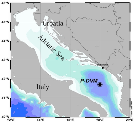
Figure 1.
Study area with a sampling station.
Vertical profiles of temperature, salinity, chlorophyll-a fluorescence (Chl-a) and dissolved oxygen (DO) concentration (averaged over 1 m intervals) were taken by CTD (Conductivity–Temperature–Depth) multiparametric probe SBE 911 plus (SEA Bird Electronics INC., USA) equipped with a WETLabs Fluorometer (factory calibrated using Thalassiosira weissflogii monoculture) and a SBE43 oxygen sensor. Meteorological data were obtained from the Croatian Meteorological and Hydrological Service.
A total of 48 zooplankton samples were collected by vertical tows using the Nansen opening–closing net with a 250-µm mesh (113 cm diameter, 380 cm length). In June, sampling started at 03:30 (early morning), at 05:30 (late morning), 13:00 (midday), 19:00 (early afternoon), 20:30 (late afternoon), and 24:00 (midnight). In February, due to different light conditions, sampling started at 04:00 (early morning), 07:00 (late morning), 12:00 (midday), 16:00 (early afternoon), 18:00 (late afternoon) and 22:30 (midnight). The following depth intervals were sampled: 0–50, 50–100, 100–200, and 200–300 m. Average hauling speed was 1 m/s. On board, samples were fixed and preserved in a seawater-formalin solution containing 4% formaldehyde buffered with CaCO3. In the laboratory, a qualitative-quantitative analysis of mesozooplankton was performed under an Olympus SZX16 stereomicroscope on subsamples ranging from 1/7 to 1/10, depending on the total sample abundance. Entire samples were examined for the identification of rare species. Taxonomic identification was performed to a species level for the majority of adults. Some groups were identified at higher taxonomic levels (e.g., copepodite stages, Oithona setigera group, which included individuals of O. setigera, O. longispina and O. atlantica, genera Copilia, Vettoria and Sapphirina, family Oncaeidae). Abundance was expressed as individuals per cubic meter (ind. m−3).
2.3. Data Analysis
WMD (Weighted Mean Depth) was calculated for adult copepods and their copepodite stages for June 2020, as well as for February 2021, according to the following equations: Ʃ(ni × zi × di)/Ʃ(ni × zi), where di is the midpoint of the depth interval of the sample i, zi is the thickness of the stratum and ni is the abundance of organisms (ind. m−3). Student’s t-tests were performed to evaluate differences between summer and winter WMD values of the most important copepod species, using STATISTICA 8.
To analyze diversity changes between layers, the Shannon–Wiener diversity index (H′) was calculated for each sample. The Shannon–Wiener index [34] evaluates how the individuals are distributed among the taxa and was determined by the equation: H′ = −Σ(Pi × (ln Pi)), where Pi is the proportion that the i-th species represent to the total number of individuals in the sampling space. Univariate biodiversity measures were calculated with PRIMER 5 for the Windows software suite [35].
The relationship among copepod species vertical distribution and abundance and environmental data were investigated using multivariate analysis with a non-metric, multidimensional scaling (NMDS) technique using the Bray–Curtis (Sørensen) distance measure. Rare taxa (<0.5 mean contribution) were excluded from the analysis. We used 2 matrices: the ‘species’ matrix had 48 stations as rows × 50 taxa as columns. The ‘environmental’ matrix had the same 48 stations as rows in the same sequential order x 4 environmental variables as columns that measured the average values for each depth stratum of temperature, salinity, Chl-a and DO. Zooplankton sampling time (day/afternoon/night/morning), month (June/February) and depth (0–50, 50–100, 100–200 and 200–300 m) were considered as categorical variables. Data were log10(N + 1) transformed. For the ordination, the final stress (a measure of the goodness-of-fit between the data and the final ordination) was examined in relation to the dimensionality to help choose the minimum number of dimensions necessary to adequately describe the data. The results are shown as bi-plot graphs (the first two ordination axes) with environmental variables as vectors and sampling stations as points in ordination space [36].
Once the main environmental variables affecting the variability of vertical and seasonal copepod abundance were identified with the NMDS technique, we used the multi-response permutation procedure (MRPP) to test several null hypotheses (Ho) that the abundance of species and zooplankton community structure differ significantly among different sample groups: daytime, winter vs. summer and among sampling depth layers. The separation between groups is determined by the Pearson type III distribution (T): the more negative the T value, the stronger the separation. The MRPP also calculates the chance corrected for within-group agreement (A): if A = 1, all items are identical within the groups (delta = 0); if A = 0, heterogeneity within the groups is expected by chance, and if A < 0, heterogeneity between the groups is higher than expected by chance [36].
The indicator species analysis (ISA) was used to identify the typical copepod species of each sampling group defined according to the null hypotheses proposed for the MRPP analysis. The ISA measures the faithfulness of the occurrence of species within a particular group station defined by a null hypothesis. Indicator values for each species can range from 0 to 100; a score of 100 means that the presence of that particular species points unequivocally to a specific group [36]. The highest indicator value for each species is tested for statistical significance using a Monte Carlo test of 1000 randomizations. The NMDS, MRPP and ISA are nonparametric tests and were conducted in PC-ORD for Windows 5.10 [37].
3. Results
3.1. Environmental Conditions
Data acquired during the two sampling cruises characterized two different environmental conditions typically associated with the summer and winter seasons (Figure 2A). In June, the temperature decreased gradually from the surface (24.05 °C) to the deeper layers, where the minimum was recorded at 300 m depth (14.53 °C). A typical seasonal thermocline was present in the upper 50 m. During February, the water column was well mixed with relatively uniform thermal conditions (average 14.47 ± 0.008 °C). Salinity values in June were relatively lower in the upper 20 m, with an average of 38.71 ± 0.04. The maximum of 38.96 was found at 60 m depth. Winter conditions showed stable salinity conditions, with a minimum recorded on the surface (38.90) and average values of 38.92 ± 0.002. Mean DO concentration was higher in June (5.32 mL L−1 O2) than in February (4.73 mL L−1 O2). In July, the highest concentrations were in the upper 80 m, with a maximum of 6.01 mL L−1 O2 at 30 m depth. This is associated with a significant increase in Chl-a (maximum of 0.46 mg m−3). Additionally, February meteorological conditions are shown since they were directly responsible for deep convection, which occurred before our sampling (Figure 2B). A strong Bura event was recorded from the 11th to 14th of February, just three days before the sampling exercise in February 2021, with wind gusts surpassing 50 m/s, coupled with a decrease in air temperature.
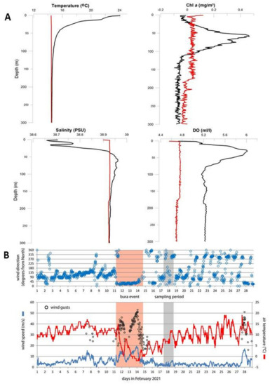
Figure 2.
Environmental parameters at the sampling station in June 2020 (black line) and February 2021 (red line) (A), and meteorological conditions in February 2021 (B).
3.2. Vertical Distribution of Copepod Abundances and Diversity
Figure 3 shows the vertical distribution of total copepod numbers (adults and copepodite stages) separated by main orders. Cyclopoida, Mormonilloida and Harpacticoida were, in general, considerably less abundant than Calanoida in both seasons.
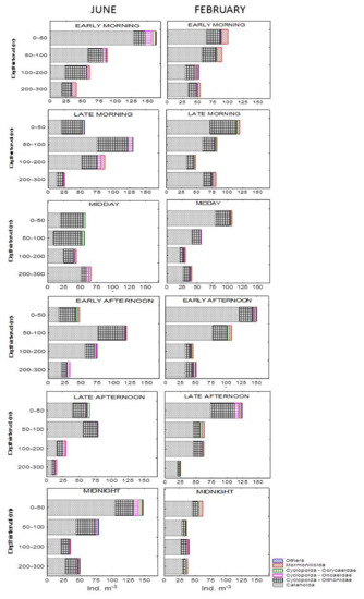
Figure 3.
Vertical distribution of copepod abundances for each sampling time and depth interval in June 2020 and February 2021.
In June, the overall mean copepod abundance was 68.9 ± 38.3 ind. m−3. In the surface layer, two peaks of abundance were recorded: in early morning (163 ind. m−3) and at midnight (147.6 ind. m−3). This layer showed the widest diel oscillations of total percentages of relative abundances, ranging from 47.2% to 18.7% at midnight and in the late morning, respectively. With increasing daylight, calanoids retreat to deeper layers. Thus, at midday, the bulk of calanoid populations were concentrated in the 200–300 m layer, with the layers above inhabited mainly by Oithonidae. Furthermore, during the midnight–early morning period, higher values of Oncaeidae (up to 10.2 ind. m−3 in the early morning) were detected at the surface. The contribution of calanoid copepodite stages to the total copepod numbers was, on average, 19% and increased up to 29% at midnight at the 100–200 m layer. Juvenile Oithona stages contributed, on average, 21%.
In February, mean copepod abundance was 69.7 ± 33.8 ind. m−3. Over the entire sampling period, the maximum overall numbers of individuals occurred in the 0–50 m layer, ranging from 149.9 to 62.5 ind. m−3, representing early afternoon and midnight values, respectively. In general, a trend toward decreasing abundance with depth was observed, with calanoids remaining the dominant group over the entire sampling period. Fewer oscillations in total percentages of relative abundances of each layer during the 24 h period were recorded than in summer sampling. Thus, the 200–300 m layer showed higher differences, ranging from 24.3% in the late morning to 9.0% in the late afternoon. Calanoid copepodite stages accounted for 24%, while Oithona copepodites accounted for 12% with respect to the entire copepod population.
In all, 87 copepod taxa were identified: 77 in June and 75 in February. The most diverse group was order Calanoida, with 64 species found. Cyclopoida was represented by the families Oithonidae (5 taxa), Oncaeidae, Lubbockiidae (one species—Lubbockia squillimana), Corycaeidae (9 species) and Saphirinnidae (genera Copilia, Sapphirina, and Vettoria). Harpaticoida included three species (Clytemnestra gracilis, Microsetella norvegica, and Macrosetella gracilis), while the order Mormonilloida included one species: Neomormonilla minor.
The highest number of taxa (40) was recorded in the surface layer (midnight) in June and the 100–200 m layer (late afternoon) in February (Figure 4). Average Shannon–Wiener diversity index was lower in July (2.21 ± 0.27) than in February (2.54 ± 0.18) and highest in the 100–200 m layer (2.46). Differences between the number of taxa found and the estimated diversity index between the two seasons were the most pronounced in deeper investigated layers, especially the 200–300 m layer, during the whole sampling period. The maximum H′ of 2.8 was found in a midnight sample from the deepest layer taken in February. In June, the wider oscillations between day and night were reported, especially in the upper layers, where we found a considerably higher number of taxa and diversity during the night and morning.
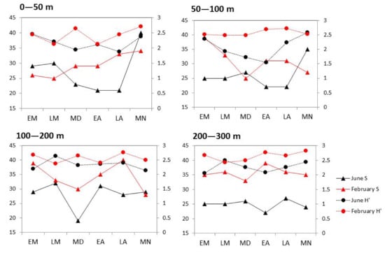
Figure 4.
Vertical distribution of the number of taxa (S, left y-axis) and Shannon–Wiener index (H′, right y-axis) for each sampling time (EM—early morning, LM—late morning, MD—midday, EA—early afternoon, LA—late afternoon, MN—midnight) at four depth layers in June 2020 (black lines) and February 2021 (red lines).
3.3. Dial and Seasonal Vertical Distribution Patterns of Dominant Copepods
Diurnal vertical abundance profiles of the taxa with a contribution greater than 1% are presented in Figure 5. The dominant copepod genera were Clausocalanus and Oithona, especially in the upper 100 m. Among the eight species of the genus Clausocalanus found in the area, those with higher abundances were: C. pergens (with a peak abundance in the surface layer at midnight (June) and late afternoon (February); C. parapergens (with a peak in late morning/early afternoon in the 0–50 and 50–100 m layers, respectively in June, and late afternoon in the 0–50 m layer in February; C. paululus (whose peak was in the surface layer of both seasons, in late morning in June and late afternoon in February) and C. mastigophorus (with considerably higher abundances recorded in February, especially in the upper 100 m during the daylight). During the strongest daylight (midday) in June, the Clausocalanus species avoided the upper 100 m depth. Furthermore, C. parapergens, C. paululus and C. mastigophorus showed distinct, although not significant, seasonal WMD variations and exhibited deeper WMD in June (Table 1). Their copepodite stages were relatively numerous in both seasons. The Oithona setigera group was more abundant in June, when, except for the surface layers during the day, they also showed higher abundances in the deeper layers over the night. O. similis was constituted by the bulk of the population occurring in the 0–100 m layer in both seasons. During June, Neomormonilla minor remained in the deeper layers, while in February, considerably higher numbers were recorded up to the surface during the night–late morning. Haloptilus longicornis showed significant seasonal variations in vertical distribution and was constituted by the bulk of the population occurring below 100 m in July. In February, this copepod was more uniformly distributed in the upper 300 m of the water column. Lucicutia flavicornis and Ctenocalanus vanus are copepods whose WMD generally did not differ between the seasons, although they had different diel patterns between seasons. L. flavicornis reached maximum abundance in the late afternoon (100–200 m) and night (0–50 m) in summer, thus avoiding surface layers during the strongest insolation. The winter peak for this species was recorded at the surface in the early afternoon. During the winter, C. vanus was consistently abundant in the 50–100 m layer. A strong migrant P. gracilis performed surface migration only in June, while during February the majority of the population remained in the 200–300 m layer. For both adults of P. gracilis and Pleuromamma copepodite stages, WMD was observed deeper during the winter mixing. Similar vertical movements were recorded for P. abdominalis as well as for another intermediate water copepod—Euchaeta acuta, performing standard DVM movements only during the stratification period. Mecynocera clausi occupied surface layers in June with a peak in the late afternoon, while during February, it was more or less evenly distributed through the investigated layers.
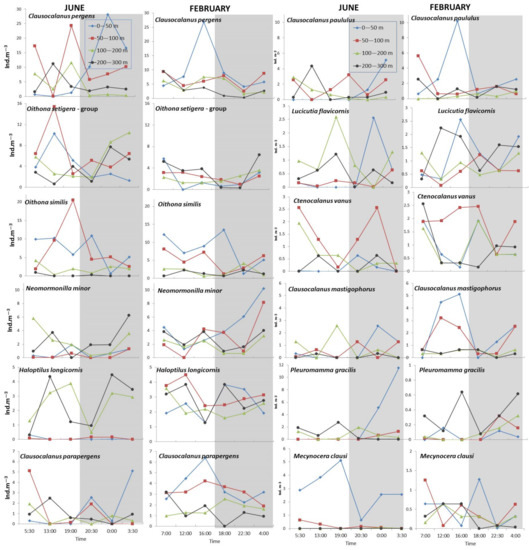
Figure 5.
Vertical distribution of the most abundant copepod taxa (with >1% contribution to total density) in four depth sampling layers at each sampling time in June 2020 and February 2021.

Table 1.
Mean abundances ± SD and Weighted Mean Depths (WMD) of the different copepod taxa (>1% mean contribution) and some of the copepodite stages in June 2020 and February 2021; t values estimated by the t-Student test are given with relative significance levels. Significant levels are given in bold.
With respect to copepods living at great depths (results not shown), Monacilla typica has not been recorded in the upper 300 m, while E. messinensis was recorded up to the surface layers in the early morning of June. The two species of the genus Spinocalanus also occurred in the upper 300 m only in June: S. longicornis only during the night, while S. oligospinosus was found sporadically in the deepest sampling layer and also at 100–200 m during the night-early morning. T. mayumbaensis was found during the night in June in the 100–200 m layer, while in February, during the late morning, this copepod was found up to the 100–50 m layer.
3.4. Environmental Drivers of the Copepod Community
The NMDS ordination resulted in an optimum two-dimensional solution with the final stress of 12.5 (p = 0.004). The two axes explained 91.6% of the total variability of the zooplankton community structure (r2 = 0.75 for axis 1 and r2 = 0.16 for axis 2). The NMDS ordination shows that the various station groups were divided according to the sampling season and sampling layers (Figure 6). Temperature and DO had the highest correlations with the first ordination axis (Table 2), reflecting the seasonal and vertical temperature gradient. This axis separates June surface samples from the June deep assemblage together with all February samples that were clustered on the left side of horizontal axis 1 in the NMDS plot. C. typicus, C. jobei, F. rostrata, T. stylifera and C. pavo are located in the right half of axis 1 ordination because they were more abundant in the summer surface samples, while genus Spinocalanus, Heterorhabus and Haloptilus were located on the left, indicating lower temperatures and high salinity values, representing a deep environment. Salinity and temperature were the environmental variables that prevailed in the vertical distribution of copepods along the second axis, separating mainly deep June samples and consequently the species that appear there.
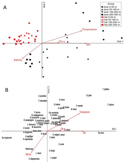
Figure 6.
Ordination joint plot from the non-metric multidimensional scaling (NMDS) of copepod abundance and four environmental variables recorded in June 2020 and February 2021 in the south Adriatic Sea. The NMDS sampling stations per layer and environmental vectors (A) and species (B) are equally oriented.
Table 2.
Results of non-metric multidimensional scaling (NMDS) analysis of the environmental conditions recorded for the station sampled per depth layer in the south Adriatic in June 2020 and February 2021. Randomization of the Monte Carlo test gave a probability (p = 0.004) that the final stress level of 12.6 could have been obtained by chance.
The MRPP showed that summer copepod assemblage was significantly different from the winter assemblage (p < 0.0000; Table 3). The ISA of these groups showed many strong indicators, especially for the winter season. Thus, there were twelve indicators for February (IV > 30; p < 0.05) and eight indicators for June (IV > 24; p < 0.05) (Table 4). The MRPP also indicates significant differences in copepod community structure between sampling depth layers (p < 0.0016). Of the eight indicators of the surface layer, Temora stylifera was also a significant indicator for the warm season and Onichocorycaeus giesbrechty for the cold season. Only Calocalanus styliremis and Ctenocalanus vanus were indicative for the 50–100 m and Heterorhabdus papilliger for the 100–200 m layer. From the three indicators of the deepest layer investigated, two of them (L. clausi and S. oligospinosus) were indicative for the June samples as well. Less differences were recorded between day and night samples, although strong migrant middle zone species were significant indicators (IV > 40; p < 0.05) for the night samples.
Table 3.
Multi-Response Permutation Procedure (MRPP) analysis for comparison of the copepod community structure per season, sampling depth layer and day–night sampling. The number of zooplankton samples per group is shown in parentheses.
Table 4.
Indicator Species Analysis (ISA) of the copepod taxa in the south Adriatic Sea during June 2020 and February 2021 according to season, sampling layer and day–night criteria. Rare taxa (<0.15 % contributions were excluded). Only copepod species with significant comparisons (p < 0.05) are shown in the table.
4. Discussion
A short sampling scale taken at two contrasting environment conditions with a detailed description of the vertical pattern of copepod abundance and species composition such as the regime used in our study is lacking for the area of the Adriatic Sea. The upper oceanic waters in June are characterized by vertical gradients of environmental factors, while in February, oceanic waters show relatively homogeneous physicochemical conditions. The February cruise took place after strong Bora wind episodes and consequent substantial winter heat loss at the air–sea interface. Therefore, we encountered the occurrence of a deep mixing, which extended up to 600 m. In June, a thermocline and halocline were observed along the water column with the vein of LIW between depths of 40 and 150 m. Winter vertical mixing enhances nutrients and phytoplankton development of the surface layers [24] and can consequently cause short outbreaks of micro and mesozooplankton densities in this system [18,20,31]. Higher concentrations of copepod developmental stages up to 300 m depth were recorded in winter 2015 as a consequence of large and rapid variations in production conditions driven by overall environmental changes and complexity of processes in the entire water column of the SA [31]. After the convective mixing in 2008, an increase in copepod density in the surface, and also in the 300–400 m layer, were registered [18]. During the winter sampling in 2021, this was not the case and our observed copepod densities in the upper 300 m were in accordance with the oligotrophic character of the area [13]. However, it seems that our winter investigation followed immediately after vertical mixing and phytoplankton (copepods’ food) had not yet developed, as we can see from Chl-a vertical distribution. In contrast, in June, the subsurface chlorophyll maximum was registered, but total copepod abundances were similar to those in February. We can suppose that the salp bloom already recorded in April and June at the open sea [23] may be responsible for hampering the development of other herbivorous zooplankton such as copepods by the strong reduction in phytoplankton. Anyhow, our estimated densities are in agreement with samples of comparable mesh sizes from the other oligotrophic areas in the Mediterranean Sea [38,39,40]. The use of a larger sampling mesh size (250 µm) may underestimate the abundance of the early developmental stages or smaller size copepods whose contribution to the overall copepod community can be significant in pelagic coastal and transitional areas [41,42,43]. Therefore, this should be taken into account during the interpretation of the quantitative copepod data. However, coarser net with a bigger mouth opening catches a greater number of larger calanoid species that occur in low densities but contribute to overall zooplankton biomass. This is especially true for the open waters where a considerable number of oceanic, larger size forms are present. Another important advantage of the mesh size used is the possibility of comparison with historical datasets where 250-µm mesh size was widely used (e.g., [15,16,44]).
The bulk of copepod concentration in Adriatic, as for the entire Mediterranean, is concentrated in the epipelagic zone with decreasing abundances with depth [44,45,46]. Generally, our results confirm that statement, although overall total copepod abundances varied over the investigated water column between the seasons and sampling time. During the winter vertical mixing, the bulk of the copepod population remained in the epipelagic zone (0–100 m) over the entire 24 h cycle, with calanoids remaining the dominant group. Diel vertical movements were characterized by the lowest numbers found at midnight, especially in the upper 50 m, suggesting a lower intensity of DVM in winter, as reported previously in the south Adriatic [15] and confirmed recently by the strength of the backscatter signal from an Acoustic Doppler Current Profiler (ADCP) [21]. By contrast, an increasing trend of copepod standing stocks from midnight to early morning in the surface layer found in June is in agreement with previous records of copepod day–night variations in the Mediterranean Sea [38,44,47,48]. A marked reduction in abundances, particularly calanoids, was recorded in the epipelagic layer (0–100 m) during the highest light intensity in June, with the center of calanoid abundances remaining relatively low (200–300 m). Thus, during the day (from the late morning to early afternoon), surface layers remained occupied by mostly smaller zooplankton members, primarily Oithonidae as well as notable numbers of another thermophilic group—Corycaeidae. Recent studies highlight the importance of genus Oithona in temperate seas and also their relative importance compared to calanoid copepods [46,49,50]. Due to their wide tolerance of temperature and salinity and opportunistic diet, Oithonidae are well adapted for the utilization of food resources in a stratified environment [51,52]. This study confirms their importance, which is even more apparent during the strongest sunlight over the stratified conditions when most of the calanoid species avoid surface layers. Similar results were found in the coastal area of the Mljet lakes, where seasonal studies on the vertical distribution of zooplankton showed that the genus Oithona was numerically dominant during the summer, with O. nana being one of the dominant zooplankton species in the surface layers during the warmest period [53]. As opposed to seasonal changes in vertical positioning, small copepods such as Oithona spp. usually show little or no DVM behavior [54].
Values of the Shannon–Wiener diversity index is in accordance with previous records for the SA [19,20], although we found a slightly lower number of species compared to the data along the east–west transect [20]. Even though historical data reported reduced numbers of copepod species found during the winter in the SA [55], recent results as well as our research indicate higher diversity over the colder part of the year [20]. The vertical patterns of diversity showed higher values in 100–200 m layers, which corresponded to the findings reported by Scotto di Carlo et al. [44] and Brugnano et al. [47] for the Tyrrenian Sea, Siokou-Frangou et al. [46] for the eastern Mediterranean basin and Zagami et al. [48] for the Ligurian Sea. Brugnano et al. [47] reported increased diversity in the 100–200 m layer in the afternoon due to the upward-moving mesopelagic copepod species. Enrichment of epipelagic waters during the night by diel migrants that ascend from the pelagic layer has been widely reported in the Mediterranean Sea [38,44,47,56]. Our day–night differences in diversity and number of taxa of the epipelagic area were more pronounced in June, which is related to higher intensity of DVM compared to February as well as deficiency of calanoids during the intensive daylight.
DVM patterns of the investigated copepod species varied between the two seasons. Many common epipelagic species such as Clausocalanus jobei, C. arcuicornis, C. vanus, and Mecynocera clausi are reported in the literature as weak or non-migrant species [44], with abundance maxima from 50 to 100 m during the day and above 50 m at night. C. paululus, C. parapergens and L. flavicornis have a wider distribution, with abundance maxima from 100 to 200 m during the day and from 50 to 100 m at night [44]. However, Brugnano et al. [47], in spring sampling of the open central Tyrrhenian Sea, did not find significant migrating behaviors of those species. Similar results were reported by Zagami et al. [48] in the Ligurian Sea, where Clausocalanus spp. were characterized by different vertical partitions, with no significant variations in the day/night WMDs. Although there are no data for their DVM in the Adriatic, our results show that for Clausocalanus spp. and L. flavicornis, nocturnal upward and diurnal downward migration were more obvious in summer when they migrate toward the food-rich areas during the night when the risk of attack is greatly reduced. C. pergens showed a pronounced descent only during the strongest sunlight, while it remains in the subsurface chlorophyll maximum layer (50–100 m) over the rest of the 24 h cycle. High backscatter values during the warmer part of the year in this layer were registered [21]. A different pattern was found during the winter mixing when those species occurred with higher abundances in the surface layer somewhat earlier (late afternoon). Of the most frequent calanoids, it seems that only M. clausi tolerate higher light intensity and showed higher densities in the surface layer, in both day and night samples, especially in summer. Our reported abundances of Neomormonilla minor are considerably higher than previously reported for the Adriatic Sea [13] sampled by the same mesh size. Records on the diel migration of N. minor in the Adriatic are missing. Interestingly, although previously reported occurrences of this species were at not more than 50 m depth [13,20], during the winter mixing, N. minor contributed significantly to the total copepod values of the upper 100 m, especially in the surface layer from midnight to early morning. Our result does not confirm previous records by Scotto di Carlo et al. [44] regarding its inverse migration. N. minor is well adapted to the oligotrophic environment [57], and it seems that during the favorable winter isothermal conditions, it can spread its vertical dispersion up to the surface layers. Mid-water copepod H. longicornis, characteristic of the oligotrophic environments [58], is known in the literature as a weak or non-migrant species [13,15,44]. Our data indicate bimodal distribution and confirm well-defined seasonal differences [15,20], with higher values found in the surface layers during the mixing period. The strong migrant P. gracilis reaches the surface between midnight and early morning in June, which is in agreement with previous studies [47,48]. Our records showed that diurnal migration of this copepod is of greater intensity in summer and confirmed its appearance at the surface during the daylight only in winter [15]. Furthermore, seasonal vertical partition of P. gracilis, as well as Pleuromamma copepodite stages, indicate a deeper preferential depth in winter and, therefore, less need to come up to feed on the surface because of more food in the deeper layers as a result of vertical mixing conditions. A similar seasonal trend was found for the other mesopelagic species (P. abdominalis, E. messinenssis, E. acuta, genus Spinocalanus), whose DVM was more intense in summer. This is in agreement with previous reports from the continental shelf station in the SA [15] as well as with data from the backscattering strength, whose maximum excursion between day and night was in summer/autumn in the 200–300 m layer [21]. Our sampling method is inadequate to show vertical migration of mesopelagic or even deep copepod species. Still, our findings of T. mayumbaensis up to the 100–200 m layer in June (night) or even the 50–100 m layer in February (early morning) indicate a shallower vertical dispersion of this species than previously recorded for the Adriatic, where it was found only below a depth of 300 m [13,15,20].
Despite different diel cycles performed by some of the species, the observed differences in total abundance of the copepod community based on MRPP analysis showed no significant separation between day and night samples. The above result is due to the absence of strong migrant species in the area, as generally reported in the other Eastern [45,46,59] and Western [44,48,60] Mediterranean areas. Thus, ISA showed only strong migrating species were indicative for the night period. Species abundance and composition were primarily differentiated according to warm and cold seasons. Thus, the copepod community was strongly affected by temperature and oxygen saturation and thus exhibits clear seasonal structuring shown in NMDS. During the warm season, distinct species-specific responses to the environmental oscillations were recorded. Thus T. stylifera, C. typicus, F. rostrata, M. clausi, C. pavo, Oithona spp. are likely to stay in the warm surface layer, while L. clausi, S. oligospinosus, C. poppei, E. acuta peaked at higher salinities but lower temperatures, thus shaping the deeper layers in summer. It is not surprising that the winter mixing period showed weak separation between the samples due to the relative homogeneity of water properties, with twelve indicators identified. The majority of Clausocalanus spp. as well as Lucicutia flavicornis was important in shaping the winter copepod community. Their seasonal vertical positioning in oligotrophic waters was characterized by occupying lower depths in summer but shallower depths for the rest of the year, as reported previously [44,61], and thus appears to successfully resist vertical currents during the connective mixing. Clausocalanus spp. is dominant in winter and, as an omnivorous genus, is particularly adapted to a wider range of food resources under the low phytoplankton concentrations [62,63]. Midwater genera Haloptilus and Heterhorabdus were important in shaping the deeper winter community.
The present study provides detailed information on the vertical distribution and diel migration patterns of the copepods in an oligotrophic environment under two contrasting hydrographical conditions. In a pelagic system, the copepod vertical zonation patterns are mainly determined by water depth, despite seasonal differences and hydrographic features [64], with competition and predation as determinants regulating the patterns within the plankton communities [65]. Depth plays an even more important role in structuring a copepod assemblage during the stratified conditions, selecting species-specific successions in relation to temperature and oxygen conditions. Thus, different vertical distribution patterns in relation to sampling hours and seasons reflect the abundance variations between the copepod species but also within the same population. General descent at sunrise to avoid strong sunlight and predators was found for most of the calanoids in summer. Thus, surface layers during the day are being inhabited by relatively small taxa: Oithona, Mecynocera clausi, as well as some less abundant species such as Temora stylifera, Centropages typicus and Calocalanus pavo. In winter, when the deepest layers receive more food than usual from the upper layers, the vertical migrations are less intense and, therefore, not mandatory behavior. Additionally, the connective mixing may cause a probably short-term appearance of the deep-water copepods (Neomormonilla minor, T. mayumbaensis) up to the upper layers. Copepod vertical migrations are complex behaviors, and the various aspects that we have considered here in this report underline the need for further detailed studies, which will include species life strategies, trophic relationships, light sensitivity, and feeding behavior, etc., that could be interesting to investigate. In addition, investigation of an integrated water column is needed for more accurate data on vertical zonation of mesopelagic strong migrant species such as Pleuromamma spp., Euchirella messinensis, Euchaeta acuta, which contribute significantly to overall copepod biomass. Long time scales (interannual) of zooplankton migratory patterns as well as integrated methods (biomass measurement or acoustic profiling) are needed for a better understanding of zooplankton distribution through the water column and thus modeling of the complex marine biochemical mechanisms.
Author Contributions
Zooplankton analysis and writing—original draft preparation, M.H.; interpretation of data of the article and discussion of the results, M.H., M.B., R.G.; writing—review and editing, M.B., R.G.; zooplankton sampling, M.H., R.G. All authors have read and agreed to the published version of the manuscript.
Funding
This research was funded by the Croatian Science Foundation under project IP-2019-04-9043 (DiVMAd).
Institutional Review Board Statement
Not applicable.
Informed Consent Statement
Not applicable.
Data Availability Statement
Not applicable.
Acknowledgments
The authors would like to thank the captain and crew members of the research vessel R/V Naše More and all the scientific and technical staff who took part in the cruises. We thank Steve Latham for the English editing of the manuscript. We also thank the anonymous reviewers for the constructive comments and valuable suggestions.
Conflicts of Interest
The authors declare no conflict of interest.
References
- Licandro, P.; Icardi, P. Basin Scale Distribution of Zooplankton in the Ligurian Sea (North-Western Mediterranean) in Late Autumn. Hydrobiologia 2009, 617, 17–40. [Google Scholar] [CrossRef]
- Hays, G.; Harris, R.; Head, R. The Vertical Nitrogen Flux Caused by Zooplankton Diel Vertical Migration. Mar. Ecol. Prog. Ser. 1997, 160, 57–62. [Google Scholar] [CrossRef]
- Schnetzer, A.; Steinberg, D. Active Transport of Particulate Organic Carbon and Nitrogen by Vertically Migrating Zooplankton in the Sargasso Sea. Mar. Ecol. Prog. Ser. 2002, 234, 71–84. [Google Scholar] [CrossRef]
- Hays, G.C. A Review of the Adaptive Significance and Ecosystem Consequences of Zooplankton Diel Vertical Migrations. In Migrations and Dispersal of Marine Organisms; Jones, M.B., Ingólfsson, A., Ólafsson, E., Helgason, G.V., Gunnarsson, K., Svavarsson, J., Eds.; Springer Netherlands: Dordrecht, The Netherlands, 2003; pp. 163–170. [Google Scholar] [CrossRef]
- Dawidowicz, P.; Pijanowska, J. Diel Vertical Migration of Aquatic Crustaceans: Adaptive Role, Underlying Mechanisms, and Ecosystem Consequences. In The Natural History of the Crustacea: Life Histories; Oxford University Press: Oxford, UK, 2018; pp. 231–256. [Google Scholar]
- Cushing, D.H. The vertical migration of planktonic crustacea. Biol. Rev. 1951, 26, 158–192. [Google Scholar] [CrossRef] [PubMed]
- Winfried, L. Ultimate Causes of Diel Vertical Migration of Zooplankton: New Evidence for the Predator-Avoidance Hypothesis. Arch. Hydrobiol. Beih. Ergeb. Limnol. 1993, 39, 79–88. [Google Scholar]
- Dale, T. Diel Patterns in Stage-Specific Vertical Migration of Calanus Finmarchicus in Habitats with Midnight Sun. ICES J. Mar. Sci. 2000, 57, 1800–1818. [Google Scholar] [CrossRef]
- Kaartvedt, S. Habitat Preference during Overwintering and Timing of Seasonal Vertical Migration of Calanus finmarchicus. Ophelia 1996, 44, 145–156. [Google Scholar] [CrossRef]
- De Robertis, A. Size-Dependent Visual Predation Risk and the Timing of Vertical Migration: An Optimization Model. Limnol. Oceanogr. 2002, 47, 925–933. [Google Scholar] [CrossRef]
- Liu, S.-H. Diel Vertical Migration of Zooplankton Following Optimal Food Intake under Predation. J. Plankton Res. 2003, 25, 1069–1077. [Google Scholar] [CrossRef][Green Version]
- Isla, A.; Scharek, R.; Latasa, M. Zooplankton Diel Vertical Migration and Contribution to Deep Active Carbon Flux in the NW Mediterranean. J. Mar. Syst. 2015, 143, 86–97. [Google Scholar] [CrossRef]
- Hure, J.; Kršinić, F. Planktonic Copepods of the Adriatic Sea. Nat. Croat. 1998, 7, 1–135. [Google Scholar]
- Hure, J. Distribution Annuelle Vertical Du Zooplankton Sur Une Station de l’Adriatique Méridionale. Acta Adriat. 1955, 7, 1–72. [Google Scholar]
- Hure, J. Dnevna Migracija i Sezonska Vertikalna Raspodjela Zooplanktona Dubljeg Mora. Acta Adriat. 1961, 9, 1–59. [Google Scholar]
- Hure, J.; Scotto di Carlo, B. Diurnal Vertical Migration of Some Deep Water Copepods in the Southern Adriatic (East Mediterranean). Pubbl. Staz. Zool. Napoli 1969, 37, 581–598. [Google Scholar]
- Hure, J.; Scotto di Carlo, B. Ripartizione Quantitative e Distribuzione Verticale Dei Copepodi Pelagici Di Profondita Su Una Stazione Nel Mar Tirreno Ed Una Nell’Adriatico Meridionale. Pubbl. Staz. Zool. Napoli 1969, 37, 51–83. [Google Scholar]
- Batistić, M.; Jasprica, N.; Carić, M.; Čalić, M.; Kovačević, V.; Garić, R.; Njire, J.; Mikuš, J.; Bobanović-Ćolić, S. Biological Evidence of a Winter Convection Event in the South Adriatic: A Phytoplankton Maximum in the Aphotic Zone. Cont. Shelf Res. 2012, 44, 57–71. [Google Scholar] [CrossRef]
- Hure, M.; Mihanović, H.; Lučić, D.; Ljubešić, Z.; Kružić, P. Mesozooplankton Spatial Distribution and Community Structure in the South Adriatic Sea during Two Winters (2015, 2016). Mar. Ecol. 2018, 39, e12488. [Google Scholar] [CrossRef]
- Hure, M.; Batistić, M.; Kovačević, V.; Bensi, M.; Garić, R. Copepod Community Structure in Pre- and Post- Winter Conditions in the Southern Adriatic Sea (NE Mediterranean). J. Mar. Sci. Eng. 2020, 8, 567. [Google Scholar] [CrossRef]
- Ursella, L.; Cardin, V.; Batistić, M.; Garić, R.; Gačić, M. Evidence of Zooplankton Vertical Migration from Continuous Southern Adriatic Buoy Current-Meter Records. Progr. Oceanogr. 2018, 167, 78–96. [Google Scholar] [CrossRef]
- Gačić, M.; Civitarese, G.; Miserocchi, S.; Cardin, V.; Crise, A.; Mauri, E. The Open-Ocean Convection in the Southern Adriatic: A Controlling Mechanism of the Spring Phytoplankton Bloom. Cont. Shelf Res. 2002, 22, 1897–1908. [Google Scholar] [CrossRef]
- Batistić, M.; Viličić, D.; Kovačević, V.; Jasprica, N.; Garić, R.; Lavigne, H.; Carić, M. Occurrence of Winter Phytoplankton Bloom in the Open Southern Adriatic: Relationship with Hydroclimatic Events in the Eastern Mediterranean. Cont. Shelf Res. 2019, 174, 12–25. [Google Scholar] [CrossRef]
- Ljubimir, S.; Jasprica, N.; Čalić, M.; Hrustić, E.; Dupčić Radić, I.; Car, A.; Batistić, M. Interannual (2009–2013) Variability of Winter-Spring Phytoplankton in the Open South Adriatic Sea: Effects of Deep Convection and Lateral Advection. Cont. Shelf Res. 2017, 143, 311–321. [Google Scholar] [CrossRef]
- Gačić, M.; Marullo, S.; Santoleri, R.; Bergamasco, A. Analysis of the Seasonal and Interannual Variability of the Sea Surface Temperature Field in the Adriatic Sea from AVHRR Data (1984-1992). J. Geophys. Res. 1997, 102, 22937–22946. [Google Scholar] [CrossRef]
- Faganeli, J.; Gačić, M.; Malej, A.; Smodlaka, N. Pelagic Organic Matter in the Adriatic Sea in Relation to Winter Hydrographic Conditions. J. Plankton Res. 1989, 11, 1129–1141. [Google Scholar] [CrossRef]
- Malanotte-Rizzoli, P.; Robinson, A.R.; Roether, W.; Manca, B.; Bergamasco, A.; Brenner, S.; Civitarese, G.; Georgopoulos, D.; Haley, P.J.; Kioroglou, S.; et al. Experiment in Eastern Mediterranean Probes Origin of Deep Water Masses. Eos Trans. AGU 1996, 77, 305. [Google Scholar] [CrossRef]
- Gačić, M.; Borzelli, G.L.E.; Civitarese, G.; Cardin, V.; Yari, S. Can Internal Processes Sustain Reversals of the Ocean Upper Circulation? The Ionian Sea Example: Internal processes and upper circulation. Geophys. Res. Lett. 2010, 37, L09608. [Google Scholar] [CrossRef]
- Vilibić, I.; Matijević, S.; Šepić, J.; Kušpilić, G. Changes in the Adriatic Oceanographic Properties Induced by the Eastern Mediterranean Transient. Biogeosciences 2012, 9, 2085–2097. [Google Scholar] [CrossRef]
- Batistić, M.; Garić, R.; Molinero, J. Interannual Variations in Adriatic Sea Zooplankton Mirror Shifts in Circulation Regimes in the Ionian Sea. Clim. Res. 2014, 61, 231–240. [Google Scholar] [CrossRef]
- Lučić, D.; Ljubešić, Z.; Babić, I.; Bosak, S.; Cetinić, I.; Vilibić, I.; Mihanović, H.; Hure, M.; Njire, J.; Lučić, P.; et al. Unusual Winter Zooplankton Bloom in the Open Southern Adriatic Sea. Turk. J. Zool. 2017, 471, 1024–1035. [Google Scholar] [CrossRef]
- Čalić, M.; Ljubimir, S.; Bosak, S.; Car, A. First Records of Two Planktonic Indo-Pacific Diatoms: Chaetoceros Bacteriastroides and C. pseudosymmetricus in the Adriatic Sea. Oceanologia 2018, 60, 101–105. [Google Scholar] [CrossRef]
- Njire, J.; Batistić, M.; Kovačević, V.; Garić, R.; Bensi, M. Tintinnid Ciliate Communities in Pre- and Post-Winter Conditions in the Southern Adriatic Sea (NE Mediterranean). Water 2019, 11, 2329. [Google Scholar] [CrossRef]
- Shannon, C.E.; Wiener, W. The Mathematical Theory of Communication; University of Illinois Press: Urbana, IL, USA, 1963. [Google Scholar]
- Clarke, K.R.; Gorley, R.N. Primer V5: User Manual/Tutorial; PRIMER-E: Plymouth, UK, 2001. [Google Scholar]
- McCune, B.; Grace, J.B. Analysis of Ecological Communities; MjM Software Design: Gleneden Beach, OR, USA, 2002. [Google Scholar]
- McCune, B.; Mefford, M.J. PC-ORD Multivariate Analysis of Ecological Data; MjM Software: Gleneden Beach, OR, USA, 2006. [Google Scholar]
- Weikert, H.; Trinkaus, S. Vertical Mesozooplankton Abundance and Distribution in the Deep Eastern Mediterranean Sea SE of Crete. J. Plankton Res. 1990, 12, 601–628. [Google Scholar] [CrossRef]
- Siokou-Frangou, I. Zooplankton Annual Cycle in a Mediterranean Coastal Area. J. Plankton Res. 1996, 18, 203–223. [Google Scholar] [CrossRef]
- Mazzocchi, M.G. Spring Mesozooplankton Communities in the Epipelagic Ionian Sea in Relation to the Eastern Mediterranean Transient. J. Geophys. Res. 2003, 108, 8114. [Google Scholar] [CrossRef]
- Bottger-Schnack, R. Vertical Structure of Small Metazoan Plankton, Especially Non-Calanoid Copepods. I. Deep Arabian Sea. J. Plankton Res. 1996, 18, 1073–1101. [Google Scholar] [CrossRef]
- Calbet, A. Annual Zooplankton Succession in Coastal NW Mediterranean Waters: The Importance of the Smaller Size Fractions. J. Plankton Res. 2001, 23, 319–331. [Google Scholar] [CrossRef]
- Pansera, M.; Granata, A.; Guglielmo, L.; Minutoli, R.; Zagami, G.; Brugnano, C. How Does Mesh-Size Selection Reshape the Description of Zooplankton Community Structure in Coastal Lakes? Estuar. Coast. Shelf Sci. 2014, 151, 221–235. [Google Scholar] [CrossRef]
- Scotto di Carlo, B.; Ianora, A.; Fresi, E.; Hure, J. Vertical Zonation Patterns for Mediterranean Copepods from the Surface to 3000 m at a Fixed Station in the Tyrrhenian Sea. J. Plankton Res. 1984, 6, 1031–1056. [Google Scholar] [CrossRef]
- Mazzocchi, M.G.; Christou, E.D.; Fragopoulu, N.; Siokou-Frangou, I. Mesozooplankton Distribution from Sicily to Cyprus (Eastern Mediterranean): I. General Aspects. Oceanol. Acta 1997, 20, 521–535. [Google Scholar]
- Siokou-Frangou, I.; Christou, E.D.; Fragopoulu, N.; Mazzocchi, M.G. Mesozooplankton Distribution from Sicily to Cyprus (Eastern Mediterranean): II. Copepod Assemblages. Oceanol. Acta 1997, 20, 537–548. [Google Scholar]
- Brugnano, C.; Granata, A.; Guglielmo, L.; Zagami, G. Spring Diel Vertical Distribution of Copepod Abundances and Diversity in the Open Central Tyrrhenian Sea (Western Mediterranean). J. Mar. Syst. 2012, 105–108, 207–220. [Google Scholar] [CrossRef]
- Zagami, G.; Granata, A.; Brugnano, C.; Minutoli, R.; Bonanzinga, V.; Guglielmo, L. Spring Copepod Vertical Zonation Pattern and Diel Migration in the Open Ligurian Sea (North-Western Mediterranean). Progr. Oceanogr. 2020, 183, 102297. [Google Scholar] [CrossRef]
- Kiorboe, T.; Nielsen, T.G. Regulation of Zooplankton Biomass and Production in a Temperate, Coastal Ecosystem. 1. Copepods. Limnol. Oceanogr. 1994, 39, 493–507. [Google Scholar] [CrossRef]
- Turner, J.T. The Importance of Small Planktonic Copepods and Their Roles in Pelagic Marine Food. Zool. Stud. 2004, 43, 255–266. [Google Scholar]
- Nakamura, Y.; Turner, J.T. Predation and Respiration by the Small Cyclopoid Copepod Oithona similisr: How Important Is Feeding on Ciliates and Heterotrophic Flagellates? J. Plankton Res. 1997, 19, 1275–1288. [Google Scholar] [CrossRef]
- Williams, J.A.; Muxagata, E. The Seasonal Abundance and Production of Oithona Nana (Copepoda:Cyclopoida) in Southampton Water. J. Plankton Res. 2006, 28, 1055–1065. [Google Scholar] [CrossRef]
- Miloslavić, M.; Lučić, D.; Žarić, M.; Gangai, B.; Onofri, I. The Importance of Vertical Habitat Gradients on Zooplankton Distribution in an Enclosed Marine Environment (South Adriatic Sea). Mar. Biol. Res. 2015, 11, 462–474. [Google Scholar] [CrossRef]
- Irigoien, X.; Conway, D.; Harris, R. Flexible Diel Vertical Migration Behaviour of Zooplankton in the Irish Sea. Mar. Ecol. Prog. Ser. 2004, 267, 85–97. [Google Scholar] [CrossRef]
- Hure, J.; Ianora, A.; Scotto di Carlo, B. Spatial and Temporal Distribution of Copepod Communities in the Adriatic Sea. J. Plankton Res. 1980, 2, 295–316. [Google Scholar] [CrossRef]
- Andersen, V. Zooplankton Community During the Transition from Spring Bloom to Oligotrophy in the Open NW Mediterranean and Effects of Wind Events. 1. Abundance and Specific Composition. J. Plankton Res. 2001, 23, 227–242. [Google Scholar] [CrossRef]
- Siokou, I.; Zervoudaki, S.; Christou, E.D. Mesozooplankton Community Distribution down to 1000 m along a Gradient of Oligotrophy in the Eastern Mediterranean Sea (Aegean Sea). J. Plankton Res. 2013, 35, 1313–1330. [Google Scholar] [CrossRef]
- Koppelmann, R.; Weikert, H. Spatial and Temporal Distribution Patterns of Deep-Sea Mesozooplankton in the Eastern Mediterranean? Indications of a Climatically Induced Shift? Mar. Ecol. 2007, 28, 259–275. [Google Scholar] [CrossRef]
- Kehayias, G.; Fragopoulu, N.; Lykakis, J. Vertical Community Structure and Ontogenetic Distribution of Chaetognaths in Upper Pelagic Waters of the Eastern Mediterranean. Mar. Biol. 1994, 119, 647–653. [Google Scholar] [CrossRef]
- Kouwenberg, J.H.M. Copepod Distribution in Relation to Seasonal Hydrographics and Spatial Structure in the North-Western Mediterranean (Golfe Du Lion). Estuar. Coast. Shelf Sci. 1994, 38, 69–90. [Google Scholar] [CrossRef]
- Peralba, À.; Mazzocchi, M.G. Vertical and Seasonal Distribution of Eight Clausocalanus Species (Copepoda: Calanoida) in Oligotrophic Waters. ICES J. Mar. Sci. 2004, 61, 645–653. [Google Scholar] [CrossRef]
- Kleppel, G.S.; Frazel, D.; Pieper, R.E. Natural Diets of Zooplankton off Southern California. Mar. Ecol. Prog. 1988, 49, 231–241. [Google Scholar] [CrossRef]
- Mazzocchi, M.G.; Paffenhöfer, G.-A. First Observations on the Biology of Clausocalanus Furcatus (Copepoda, Calanoida). J. Plankton Res. 1998, 20, 331–342. [Google Scholar] [CrossRef]
- Cummings, J.A. Habitat Dimensions of Calanoid Copepods in the Western Gulf of Mexico. J. Mar. Res. 1984, 42, 163–188. [Google Scholar] [CrossRef]
- Frederiksen, M.; Edwards, M.; Richardson, A.J.; Halliday, N.C.; Wanless, S. From Plankton to Top Predators: Bottom-up Control of a Marine Food Web across Four Trophic Levels. J. Anim. Ecol. 2006, 75, 1259–1268. [Google Scholar] [CrossRef]
Publisher’s Note: MDPI stays neutral with regard to jurisdictional claims in published maps and institutional affiliations. |
© 2022 by the authors. Licensee MDPI, Basel, Switzerland. This article is an open access article distributed under the terms and conditions of the Creative Commons Attribution (CC BY) license (https://creativecommons.org/licenses/by/4.0/).