Crop Water Productivity, Applied Water Productivity and Economic Decision Making

Abstract

Increasing productive water use in agriculture is seen as paramount to meet future food demand with limited water supplies. The main objective of this paper is to gain a better understanding of the interrelated linkages between crop water productivity (CWP) and applied water productivity (AWP) as affected by irrigation management decisions in order to assess the impact of economic decision making on CWP and AWP under area-limiting and water-limiting conditions. A daily soil water balance mathematical programming model that explicitly models the impact of technology choice and stochastic weather on water use efficiency was used to study the interactions. The assumption is made that a rational decision maker will allocate water to maximize expected profits. The results showed that CWP is, to a large extent, unresponsive to increasing irrigation water applications, especially when water applications are approaching maximum potential crop yields. The difference between optimal crop yields for the area-limiting and water-limiting scenarios is small, which shows that the portion of water production function that is relevant for economic decision making is small and falls within the unresponsive range of CWP changes. Profit maximizing decision makers will not try to maximize CWP or AWP since these objectives will result in profit losses.

1. Introduction

Increasing water productivity in the agricultural sector is a priority for many governments seeking to increase crop production to meet future food demands with limited water supplies [1,2]. Intuitively the objective of increasing crop water productivity (CWP), where CWP is defined as the ratio of crop yield divided by water consumed, seems sound. However, the objective of maximizing CWP to cope with water shortages has received several criticisms from a management point of view [3,4,5,6]. Van Halsema and Vincent [7] argue that the concept of water productivity has led to confusion and questionable inductions when the denominator (water consumed) is confused with applied water. An example is the work of Amarasinghe and Smakhtin [8], who sought a theoretical underpinning for the concept of a crop water footprint (inverse ratio of CWP) using the classical production function taught in production economics. The problem is that the crop water footprint requires a production function where crop yield is a function of evapotranspiration (ET), in contrast to the classical production function where crop yield is a function of applied irrigation water.

A well-established fact in literature is that the relationship between crop yield and consumptively used water (ET) is linear [9,10,11]. Doorenbos and Kassam [12] expressed the crop water production function (CWPF) on a relative basis, where the yield response factor (Ky) represents the slope of the linear relationship between relative ET deficits and relative crop yield reduction on a seasonal basis. Several researchers recognized that the effects of ET deficits in different crop growth stages on crop yield are different, and different additive and multiplicative functions have been developed to estimate the combined effects of growth stage-specific ET deficits on crop yield [13,14]. Since CWPFs are based on ET, these functions are more or less independent of the irrigation systems, soils, and other factors that influence management of applied irrigation water [15]. In contrast, the water production function (WPF) represents the non-linear relationship between yield and applied irrigation water [11,15,16]. The non-linear relationship is the direct result of the timing of water applications, amount of water applied in relation to the soil water status at the time of irrigation, and choice of irrigation technology, which results in deep percolation or runoff [11,15,16]. Thus, the relationship is much more dependent on technology choice and management.

Managing limited water supplies economically implies explicit consideration of the costs, revenues, and opportunity costs of water and requires information regarding crop yield response to ET deficits, in addition to managing field water supply to satisfy ET requirements of the crop [15]. Calculations of productivity measures based on the CWPF and the WPF are therefore interrelated for a specific technology set. Keller and Seckler [3] argue that a thorough understanding of the processes governing crop growth as a function of ET and crop growth as influenced by available water supply is critical to the evaluation of water productivity in crop production. From an economic decision-making point of view, maximizing CWP to cope with water scarcity may be inappropriate since it does not consider economic decision-making principles [6]. Consequently, the theoretical underpinning of the maximization of CWP as a criterion to cope with water shortages is weak [5]. The contrasting views regarding the applicability of using the concept of “maximizing CWP” to cope with water shortages shows that the impact of using irrigation water economically on crop water productivity (CWP) derived from the CWPF and applied water productivity (AWP) derived from the WPF is not well understood. Given the importance that governments place on increasing water productivity in agriculture, a better understanding of the interrelated linkages between CWP, AWP, and economic decision making is perceived to be critical to enhance decision support considering the use of mathematical programming models.

A general lack of understanding of the interrelated linkages between CWP, AWP, and economic decision making may result in management decisions under water-limiting and area-limiting conditions with unintended consequences on crop water productivity and profitability.

Economic management of irrigation water may require some form of deficit irrigation where the crop is deliberately under-irrigated, resulting in crop yields below maximum potential crop yield [15]. A popular method to incorporate the effects of water deficits on crop yield into mathematical programming models is the use of relative evapotranspiration formulae that relate relative ET deficits to relative yield reductions [17,18,19]. Calculating ET deficits is complex since irrigators do not have direct control over ET, but have indirect control through application of irrigation water. Not all the irrigation water that is applied is consumed due to inefficiencies resulting from deep percolation and runoff [3]. Inefficient irrigation water applications are incorporated into mathematical programming models with varying degrees of sophistication. The simplest method is to assume constant efficiencies irrespective of the level of deficit irrigation [17,20] or to assume a specific level of inefficiency in accordance to the level of water availability in relation to the required amount [21]. Assuming constant efficiencies is unrealistic because deficit irrigation reduces deep percolation and runoff losses, and consequently deficit irrigation increases water application efficiencies [16]. Some researchers [22,23] have developed seasonal production functions that incorporate non-uniform water applications to model increasing efficiencies associated with deficit irrigation. However, seasonal relationships do not allow for the effect of intra-seasonal management decisions on crop water use.

The impact of intra-seasonal management decisions on crop water use is best quantified using daily soil water balance calculations. A further benefit of using daily calculations is that the impact of stochastic rainfall events on crop water use can be explicitly modeled. Grové [24] showed that popularly available methods to incorporate daily water budget calculations into mathematical programming models may malfunction under limited water supply conditions.

Venter and Grové [25] developed an irrigation water use optimization model (SWIP) that utilizes multiple water balances to model inefficiencies conditionally on soil water status. The model optimizes the timing and amount of irrigation decisions as a function of the soil water content in relation to a critical soil water content below which ET is reduced. ET deficits are related to crop yield using the Stewart multiplicative model. Consequently, the SWIP model provides the necessary integration between the yield as a function of ET, and yield as a function of the applied irrigation water functions necessary to evaluate the impact of economic management of irrigation water on CWP and AWP. However, the model does not satisfactorily represent growing conditions in situations where rainfall contributes towards satisfying crop water requirements because the model is deterministic. By implication, the state of nature is known at the beginning of the optimization. Consequently, optimized irrigation schedules are unrealistic because the irrigation schedule will be optimized to make maximum use of rainfall.

The main objective of this study was to evaluate whether maximizing CWP or AWP is an economically rational decision-making objective when water is the most limiting production factor or when area is the most limiting production factor. The objective is achieved through the further development of the SWIP model to optimize irrigation water use while considering stochastic weather. The interrelated linkages between CWP and AWP as affected by irrigation management decisions are complex. CWP and AWP changes derived respectively from the CWPF and WPF models embedded in the SWIP model were evaluated first before determining the impact of economic decision making on productivity changes.

The paper proceeds by discussing the data and mathematical specification of the CWPF and WPF models necessary to quantify the impact of economic decision making on water productivity changes with the stochastic SWIP model, followed by a discussion of the results.

2. Data

The analyses are based on the optimization of water use of maize cultivated in Vaalharts on a soil having a water holding capacity of 120 mm/m, using a center pivot of 31.2 ha having an application rate of 12 mm/day and a coefficient of uniformity of 88%. The parameters for calculating the crop water requirements were taken from SAPWAT software [26] which is entirely based on the calculation procedures in Allen et al. [27]. SAPWAT includes 50 years of daily weather data and locally validated parameters to calculate crop water requirements for South Africa. The parameters to characterize yield response to water deficits originate from Doorenbos and Kassam [12].

2.1. Reference Evapotranspiration (ET₀)

Reference crop evapotranspiration is one of the critical inputs used to calculate crop water use because it is basically influenced by main weather factors of crop production under conditions of no water stress. ET₀ can be computed from the weather data from a specific location to understand the “evaporative” demand of the atmosphere independently of crop type, crop development, and management practices [27]. The purpose of ET₀ is to assist farmers with irrigation planning and scheduling by incorporating the crop coefficients (Kc) to determine maximum/potential evapotranspiration of a specific crop. However, the use of inappropriate weather data results in overestimation or underestimation of ET₀. Figure 1 shows the average weekly ET₀ over the 49-year period as quantiles for the maize crop over a 20-week growing season.

Each week represents an average daily ET₀ for that week and quantiles are used to demonstrate ET₀ variability over the maize growing season. The general trend over the whole growing season shows that evaporative demand is highest for the first six weeks of the production season, after which it decreases towards the end of the growing season. The distribution of ET₀ between Q25% and maximum daily ET₀ appears to be narrow bounded, whereas the minimum values are far below Q25%. Furthermore, the minimum values show more erratic changes from week to week when compared to the other quantiles.

2.2. Evapotranspiration (ETm)

The distribution of weekly average daily maximum evapotranspiration (ET_m) over the growing maize season is depicted in Figure 2.

The maximum evapotranspiration (ET_m) of maize in Vaalharts was calculated by multiplying ET₀ with the growth stage-specific Kc values. The following Kc values with the length of the stages in parenthesis—0.38 (30), 0.78 (29), 1.14 (51), and 1.14 (10)—were respectively used for the four growth stages. The purpose of Kc is to describe the crop growth behavior and how the growth is related to water use. Figure 2 shows that ET_m is lowest at the beginning of the growing season even though ET₀ is highest. ET_m is highest at the end of the crop development stage. After the crop is fully developed, ET_m shows a steady decline because ET₀ is declining. The variability in ET_m is highest during crop development and mid growing stages.

2.3. Rainfall

The rain season in the Vaalharts area is usually from October to March [28]. Figure 3 shows the weekly average rainfall within the 49-year period over the 20-week maize growing season.

Figure 3 shows that the distribution of rainfall is heavily skewed. The minimum and Q25% quantile rainfall are not reflected on Figure 3 because there is 50% likelihood that rainfall will be zero or less than 1.6 mm. Care should be taken not to conclude that rainfall does not contribute significantly toward satisfying crop water demand when considering that there is a 75% chance that the average daily rainfall in any week will be below 5 mm. On average, rainfall over the 20-week growing season amounts to a total of 283 mm. The maximum daily rainfall of about 40 mm occurs in week 13. The probability of such a rainfall event occurring is, however, very small (1/49).

2.4. Available Soil Water

Domínguez [29] relates the portion (p) of total available water (TAM) that can be extracted without any crop water stress (RAM) to the maize crop’s evaporative demand as follows:

$$p=1-\left(\frac{0.606}{1+11.86e^{-\left(0.602{\mathrm{ET}}_{\mathrm{m}}\right)}}\right)$$

(1)

Figure 4 shows the average daily total available moisture and readily available moisture for a period of 49 years over the growing season of maize.

Each week represents an average daily readily available moisture (RAM) for that week and quantiles are used again to demonstrate the RAM variability over the maize growing season. The distribution of RAM in Figure 4 includes the total available moisture (TAM) as a reference point. The first four weeks of production seems to be constant and narrowly bounded at the minimum value. At the beginning of the developing stage when roots start to grow rapidly, RAM and TAM start to increase, with TAM been higher than RAM. The highest variability in RAM occurs during the development stage and mid growth season, whereas TAM reaches a maximum of 182 mm in the last two growth stages.

2.5. Economic Parameters

Economic parameters are grouped into four components, namely, production income, yield dependent cost, area dependent cost, and irrigation dependent cost. The characterization of economic parameters is made to correctly model changes in production income and costs resulting from deficit irrigation under the water-limiting and area-limiting cases.

The price of maize (ZAR 2020/ton), area dependent costs (ZAR 10,327.99/ha), and yield dependent costs (ZAR 778/ton) were sourced from the enterprise budgets published by the local co-operative. Yield dependent costs comprise changes in harvesting costs and fertilizer costs. Irrigation dependent costs are for a center pivot of 30.1 ha with an application rate of 12 mm/day. Irrigation dependent costs comprise electricity costs, labor costs, repair and maintenance costs, and the water tariff paid to the water user association. The technical coefficients used to calculate irrigation dependent costs were taken from Venter and Grové [25].

3. Mathematical Programming Models

3.1. Crop Water Production Function Model

The mathematical programming model that was used to derive the optimal CWPF is based on the Stewart multiplicative model due to its widespread use in crop water use analyses [25,29,30]. The optimization model maximizes maize crop yield based on the optimal distribution of ET deficits across crop growth stages. The convention whereby variables are presented by upper case and data parameters by lower case is followed to specify the models. The complete CWPF model specification is as follows:

$$MAX:Y_a=y_m\times {\prod }_{g=1}^4\left\{1-k{y}_g\left[1-\left(\frac{{\sum }_{t\in g}^{}ET{a}_t}{{\sum }_{t\in g}^{}et{m}_t}\right)\right]\right\}$$

(2)

Subject to:

$$ET{a}_t\le et{m}_t$$

(3)

$${\sum }_{t\in g}^{}ET{a}_t\le {\sum }_{t\in g}^{}et{m}_t$$

(4)

$${\sum }_{t\in g}^{}ET{a}_t\ge 0.5\times {\sum }_{t\in g}^{}et{m}_t$$

(5)

$${\sum }_t^{}ET{a}_t \le etmax$$

(6)

$Y_a$ and $y_m$ are, respectively, the optimised actual yield and potential crop yield in ton/ha, whereas $ETa$ and $etm$, respectively, are the actual and potential evapotranspiration on a specific day (t) within a specific crop growth stage (g) in mm. The sensitivity of the crop to relative $ETa$ deficits in each of the four crop growth stages is accounted for by the growth stage-specific yield response factor ($k{y}_g$). The multiplicative nature of the function ensures that a more-than-proportional yield reduction is modeled if $ETa$ deficits occur in more than one crop growth stage. Proper working of the model requires that daily calculated $ETa$ values are less than or equal to $etm$, which is enforced with Constraint (3), while Constraint (4) models the condition for each growth stage. The scenario in which $ETa$ deficits in excess of 50% [12] in a specific stage are not allowed is then enforced with Constraint (5). The optimal CWPF function is derived through the parameterization of $etmax$ between zero and the maximum amount of $ETa$ necessary to give a potential maize yield of 15 ton/ha.

3.2. Water Production Function Model

The WPF is derived using the same yield function as the CWPF model; however, the calculation of $ETa$ is much more complex because it is dependent on daily soil water content, which requires daily water balance calculations. The water budget calculations of the CWPF model conforms to the internationally accepted procedures to determine crop water use under soil water stress conditions [27]. To increase the realism of the optimized irrigation schedules, irrigation schedules were optimized given uncertain reference evapotranspiration and rainfall through the inclusion of six states of nature that were identified from the historical weather data using cluster analysis. Non-uniform water applications were modeled explicitly by replicating the water budget calculations for different irrigation applications across the irrigation field.

The objective of the WPF model is to maximize the average maize yield across states of nature by changing irrigation quantities. The complete specification of the model is as follows:

$$MAX:A{Y}_a={\sum }_w^{}\left({\sum }_r^{}{p}_r\times y_{m r}\times {\prod }_{g=1}^4\left\{1-k{y}_g\left[1-\left(\frac{{\sum }_{t\in g}^{}ET{a}_{r,t,w}}{{\sum }_{t\in g}^{}et{m}_{r,t}}\right)\right]\right\}\right)/3$$

(7)

Subject to:

$$ET{a}_{r,t,w}=min|\begin{array}{l}et{m}_{r,t}\hfill \\ et{m}_{r,t}\left(\frac{RW{C}_{r,t,w}}{trw{c}_{r,t}}\right)\hfill \end{array}$$

(8)

$$RW{C}_{r,t,w}=min|\begin{array}{l}rwca{p}_t\hfill \\ RW{C}_{r,t-1,w}-ET{a}_{r,t,w}+R_{r,t-1}+I{R}_{t-1}s{f}_w+T{R}_{r,t,w}\hfill \end{array}$$

(9)

$$BRW{C}_{r,t,w}=min|\begin{array}{l}brwca{p}_t\hfill \\ BRW{C}_{r,t-1,w}+B{R}_{r,t,w}-T{R}_{r,t,w}\hfill \end{array}$$

(10)

$$B{R}_{r,t,w}=max|\begin{array}{l}0\hfill \\ RW{C}_{r,t-1,w}-ET{a}_{r,t,w}+R_{r,t-1}+I{R}_{t-1}s{f}_w+T{R}_{r,t,w}-rwca{p}_t\hfill \end{array}$$

(11)

$$T{R}_{r,t,w}=r{g}_{t}BRW{C}_{r,t,w}$$

(12)

$${\sum }_t^{}I{R}_t\le alloc$$

(13)

Equation (7) shows that maize yield is calculated the same way as with the CWPF model, with the exception that $ETa$ on a specific day $\left(t\right)$ is now also dependent on the state of nature ($r$) and the water balance representing non-uniform irrigation applications ($w$). $etm$ on day $t$ is only dependent on the state of nature. The part in brackets (outer) calculates the weighted average yield across states of nature for each $w$ based on the probability ($p_r$) that state of nature $r$ will occur. The average yield over all the non-uniform water applications represents the average maize yield ($A{Y}_a$) of the irrigation strategy. In this application, non-uniform water applications were modeled with three distinct water budgets.

Equation (8) shows that $ETa$ will be adjusted downwards from its maximum potential level if the water content in the root zone ($RWC$) is below a specific threshold water content ($trwc$). $ETa$ is therefore a function of $RWC$. $RWC$ is calculated with Equation (9) as the minimum of the maximum water that could be stored in the root zone ($rwcap$) or the resulting water content balance resulting from the addition of water through irrigation ($IR$), rainfall ($R$), or the change in soil water content due to root growth ($TR$) and the loss of water through $ETa$ before percolation occurs. The impact of non-uniform irrigation applications on the water balance is modeled by adjusting the average level of $IR$ with a scaling factor ($sf$) based on the distribution uniformity of the irrigation system [24]. Consequently, the water budget calculations in each state of nature need to be replicated three times to ensure that a third of the irrigation field is under-irrigated and a third is over-irrigated. Equation (9) implicitly ensures that percolation water is lost because $RWC$ is capped at $rwcap$. $TR$ represents the amount of water that is added to the root zone as the roots penetrate the zone below the roots, and is therefore a function of the daily root growth rate ($rg$) and the water content of the layer below the roots ($BRWC$). $BRWC$ is calculated as the minimum of the amount of water that could be stored in the zone ($brwcap$) and the resulting water balance of the zone through the edition of percolation water out of the root zone ($BR$) and $TR$. $BR$ is either zero or the amount of water in excess of $rwcap$. Calculating water balance variables as the minimum of two values cause the constraints to be discontinuous. The problem is solved using a square root approximation of the minimum function [24].

The optimal WPF function is derived through the parameterization of $alloc$ between zero and the maximum seasonal irrigation amount necessary to give a potential maize yield of 15 ton/ha under non-uniform irrigation applications.

3.3. Economic Water Allocation Model

The objective of the economic water allocation model is to optimize the expected gross margin variability for a specific level of water availability by incorporating economic parameters into the water production function model developed in the previous section. The objective function of the economic water allocation model included in the water production function model is as follows:

$$MAS=\left(py\times AYa-{\sum }_t^{}I{R}_t\times idc-ydc\times AYa-adc\right)HA$$

(14)

where $MAS$ is the margin above specified costs calculated for the total irrigated area in ZAR. The calculation in parenthesis represents the calculation of $MAS$ on a per hectare basis, which is multiplied with the area irrigated ($HA$) to determine MAS for the total area. Multiplying the area irrigated with the per hectare $MAS$ calculation in the objective function ensures that the interaction between intensification of production through irrigation applications and extensification of production through changes in areas irrigated is accounted for. Production income is generated by multiplying the price of maize ($py$) in rand per ton with the average maize yield ($AYa$) in tons per ha calculated with the WPF model. The $MAS$ calculation is differentiated for costs that are dependent on yield ($ydc$) in rand/ton, irrigation applications ($idc$) in ZAR/mm on one hectare and the area irrigated ($adc$) in ZAR/ha. Irrigation dependent costs consist of electricity costs, labour costs, repair and maintenance costs, and the water tariff. The most important costs that vary with crop yield are fertilizer costs and harvesting costs, which are assumed to change linearly with changes in crop yield. Cost components that change based on the area irrigated include mechanization, fuel, seed, pest and disease control, and labor costs that are not allocated to irrigation.

The optimal economic allocation of water is evaluated through the parameterization of $alloc$ between zero and the maximum seasonal irrigation amount necessary to give a potential maize yield of 15 ton/ha under non-uniform irrigation applications.

4. Results

4.1. Crop Water Productivity

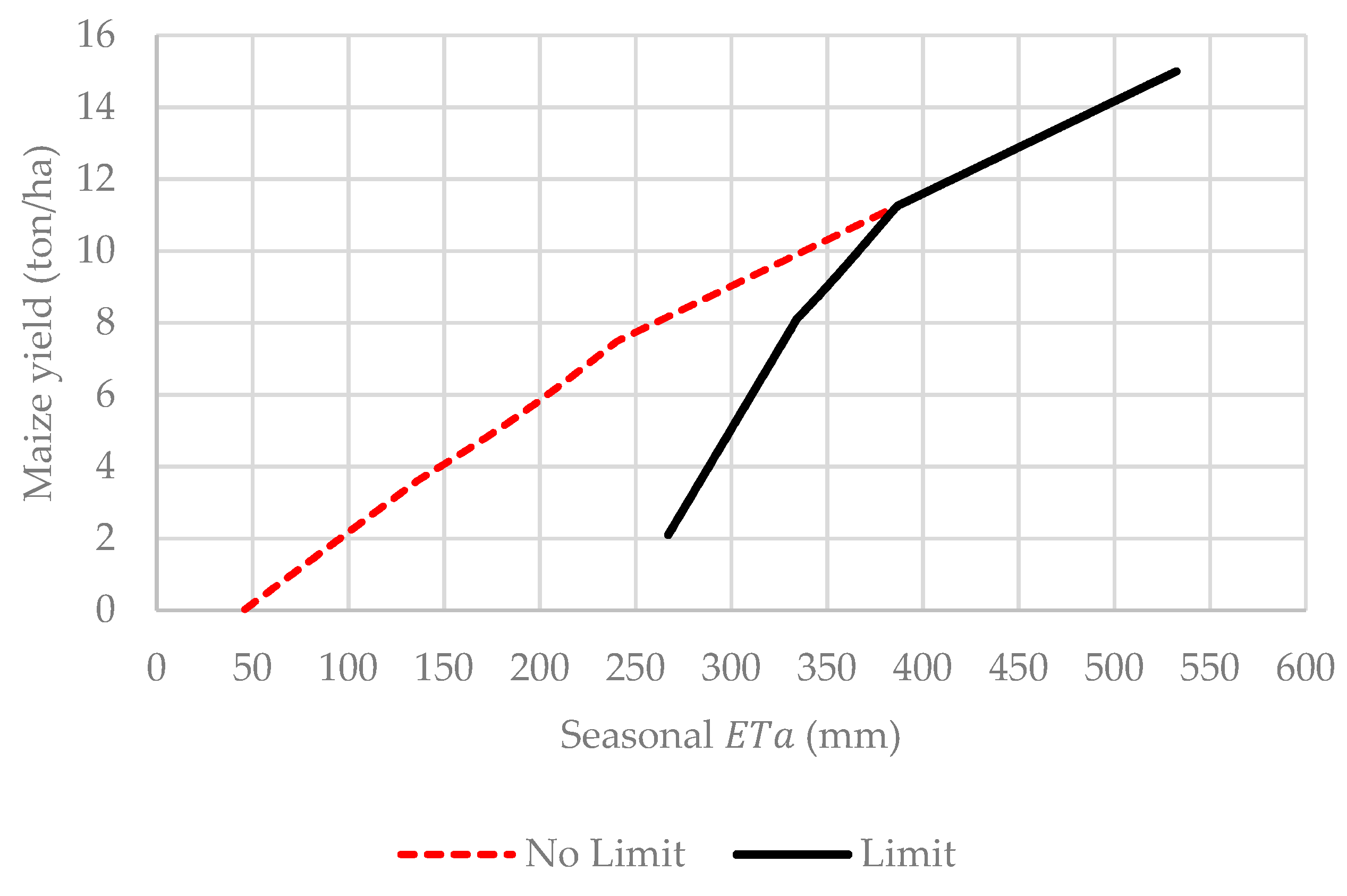
Maize yield as a function of $ETa$ as defined by the Stewart multiplicative crop water production function is discussed first, before discussing crop water productivity. Figure 5 shows the crop water production function for optimally distributed $ETa$ deficits across growth stages with a maximum $ETa$ deficit of 50% in each growth stage and no limit on $ETa$ deficits. Doorenbos and Kassam [12] stated that the linear relationship between $ETa$ deficits and crop yield does not hold for $ETa$ deficits greater than 50%. An analysis with no limit on $ETa$ deficits is therefore included to demonstrate the impact of disregarding the advice of Doorenbos and Kassam [12], as many researchers have done [20,31].

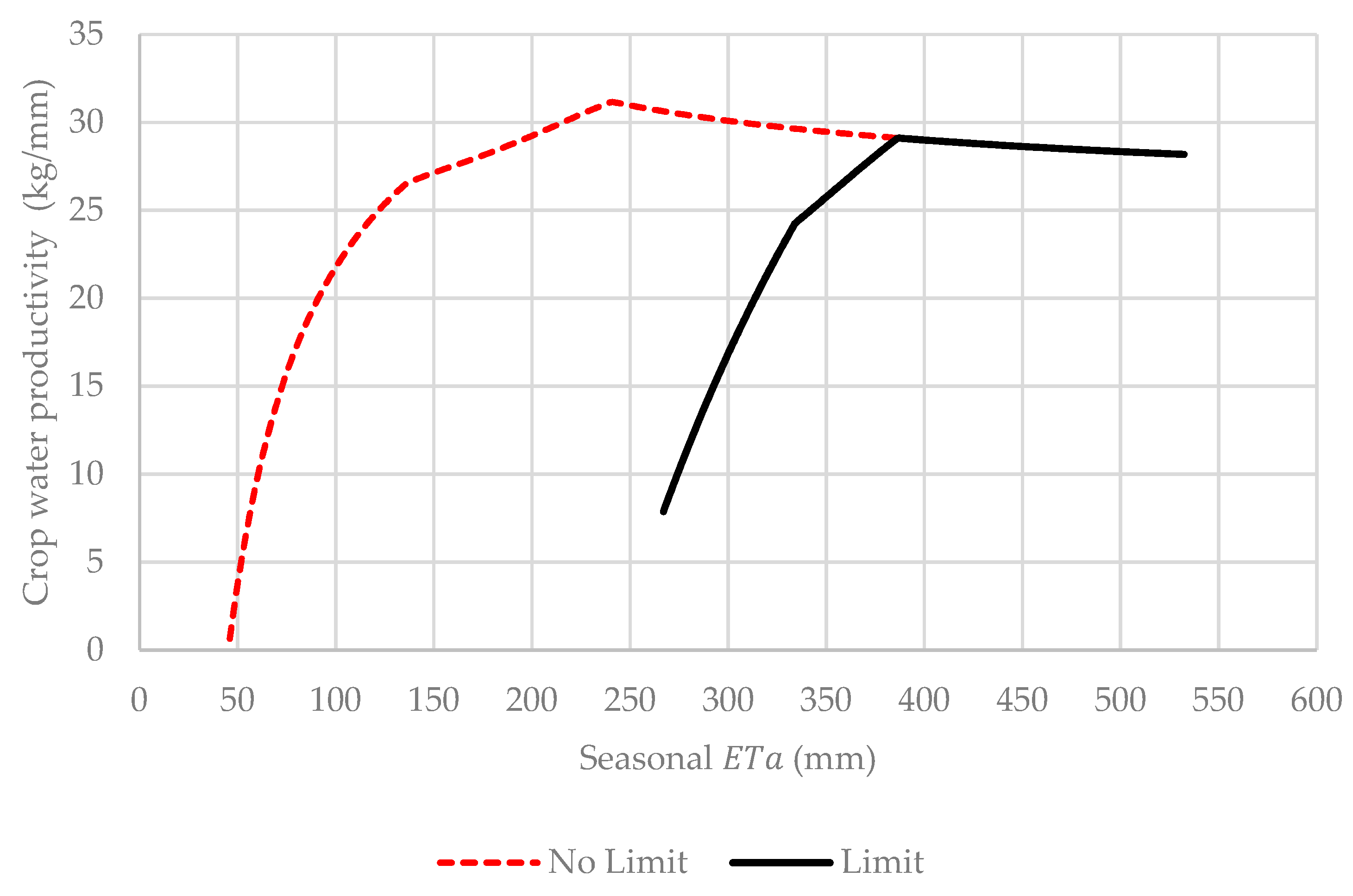
When no limit on $ETa$ deficits is enforced, it is optimal to practice deficit irrigation in one crop growth stage. Consequently, the last part of the CWPF above an $ETa$ of 240 mm is characterized by $ETa$ deficits (292 mm) in only one crop growth stage. Applying a maximum limit of 50% on $ETa$ deficits limits the amount of the $ETa$ deficit to 146 mm, before combining the $ETa$ deficits with $ETa$ deficits in other crop growth stages. Combining $ETa$ deficits in more than one crop growth stage causes crop yield to decrease more than proportionally. Overall, the limit of 50% $ETa$ deficit causes $ETa$ deficits in different crop growth stages to be combined more quickly, and therefore crop yield decreases more with increasing levels of seasonal $ETa$ deficits. The limit furthermore requires that the crop evapotranspires at least 267 mm of water to realize a crop yield. Enforcing a limit on the level of $ETa$ deficits has some serious implications for maximizing CWP.

Figure 6 shows the calculated CWP for the Stewart multiplicative CWPF with and without a limit on the level of $ETa$ deficits in a specific crop growth stage.

Figure 6 shows that the Stewart multiplicative CWPF exhibits two distinct phases of productivity changes, irrespective of whether the 50% limit on $ETa$ deficits is applied. During the first phase, CWP increases rapidly to a maximum, after which CWP decreases slowly in the second phase up to maximum potential $ETa$. CWP is maximized when no $ETa$ deficit limit is enforced and when $ETa$ is equal to 240 mm with corresponding CWP of 31.15 kg/mm. Enforcing a 50% limit on $ETa$ deficits causes the CWP maximizing level of $ETa$ to increase to 386 mm with a corresponding CWP of 29.11 kg/mm. The maize yields corresponding to maximum CWP are, respectively, 7.47 and 11.22 ton/ha when no limit on $ETa$ is enforced and when the limit of 50% is enforced. Contrarily to crop yield changes, the difference between maximum CWP and the CWP at maximum potential $ETa$ is relatively small. The impact of the 50% $ETa$ deficit limit on crop yield is therefore more amplified when compared to CWP.

4.2. Applied Water Productivity

An irrigation farmer controls the level of $ETa$ by managing the amount of available water in the root zone. Not all the water that is applied is consumptively used by the crop since some water is lost because of deep percolation, runoff, or wind drift when irrigating with a center pivot. In this research, inefficiencies are incorporated as a function of the uniformity with which water is applied. Furthermore, the amount and timing of rainfall events may significantly impact the relationship between applied irrigation water and crop yield. 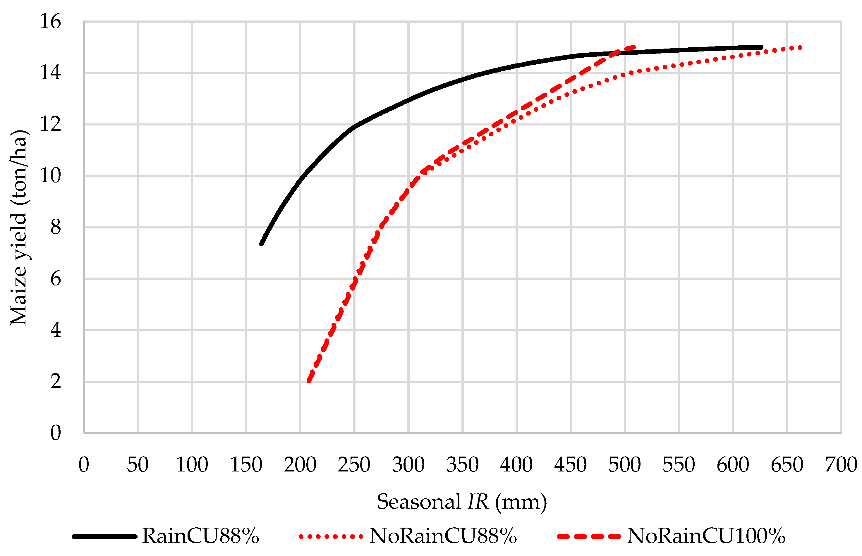Figure 7 presents the relationship between applied irrigation water for a uniform and a non-uniform irrigation application while considering rainfall or not with an $ETa$ deficit limit of 50%.

Let us consider the impact of taking account of the uniformity with which the irrigation system applies water while ignoring the contribution of rainfall first. Figure 7 shows that when the irrigation system is assumed to apply water 100% uniformly and rainfall is not accounted for, the maize WPF mimics the shape of the CWPF for the same scenario. Interestingly, the amount of water applied is constantly less than $ETa$ for the same crop yield. The amount of $ETa$ not supplied through irrigation comes from the soil water that is available to the crop at the beginning of the season. Taking non-uniformity of water applications into account while disregarding the effect of rainfall requires more irrigation to realize the same crop yield due to deep percolation losses resulting from non-uniform water applications. Consequently, 669 mm of irrigation is necessary to achieve the potential maize yield of 15 ton/ha compared to only 508 mm when the uniformity of irrigation applications is ignored. Deficit irrigation causes the soil to be dryer, which reduces the probability that some part of the field will be over-irrigated. Consequently, the difference between the two WPFs becomes less with increasing levels of deficit irrigation. For irrigation applications less than 310 mm, no water is lost through deep percolation and the two functions collapse into one function.

The WPF that accounts for both rainfall and non-uniform irrigation water applications is the average response optimized across different states of nature. Thus, effective rainfall is a function of the amount of water in the root zone, which causes inefficiencies. The WPF shows a much smoother response with a flatter slope when compared to the corresponding scenario without rainfall. The difference in crop yield at a specific irrigation water application level for the NoRain and Rain scenarios is an indication of the contribution of rainfall to the production process. At low water application levels, the contribution of rainfall is large. The contribution of rainfall becomes less important with increasing levels of irrigation because the probability that water may percolate below the root zone increases. The scenario shows that water applications can be reduced to a large extent without significantly reducing crop yields.

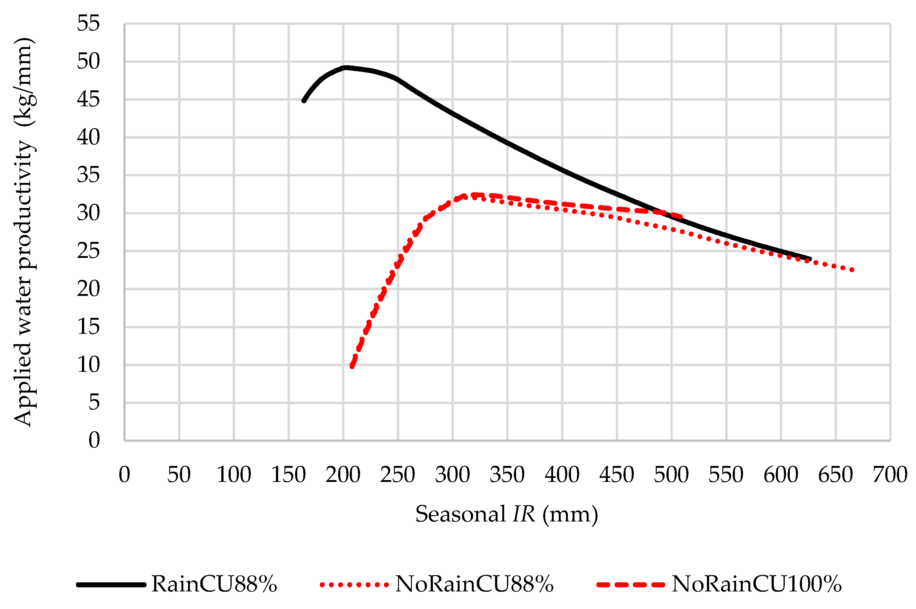
The water productivity of applied irrigation is shown in Figure 8 for uniform and non-uniform irrigation applications while considering rainfall or not with a growth stage-specific maximum $ETa$ deficit limit of 50%.

The changes in AWP portrayed in Figure 8 exhibit the same phases that characterize CWP changes. Again, let us consider the impact of non-uniform water applications while ignoring the impact of rainfall first. As expected, the AWP of the uniform and non-uniform irrigation applications are the same because the AWPFs for the two scenarios are the same if less than 310 mm of water is applied. Interestingly, this is also the irrigation amount that signifies the maximization of AWP for these two scenarios. The AWP of the non-uniform irrigation applications decreases more rapidly as a result of larger inefficiencies associated with non-uniform water applications. AWP continues to decrease from the maximum level until it reaches the application rate at which the potential crop yield is achieved. Consequently, the AWP of non-uniform water applications are much lower than uniform water applications because more water needs to be applied to achieve maximum potential crop yield.

Rainfall increases the productivity of irrigation water applications. The difference between the NoRain and Rain scenarios provides an indication of the extent of the increases. The impact of rainfall is most significant at low irrigation levels because the overall contribution of irrigation water to satisfying the requirement is relatively low compared to the contribution of rainfall. The AWP in the presence of rainfall is maximized at an irrigation application rate of 203 mm, which is almost 107 mm less than when rainfall is ignored. The fact that AWP increases before decreasing shows that rainfall alone cannot satisfy the 50% $ETa$ deficit imposed in the optimization model.

4.3. Crop Water Productivity as a Function of Applied Water

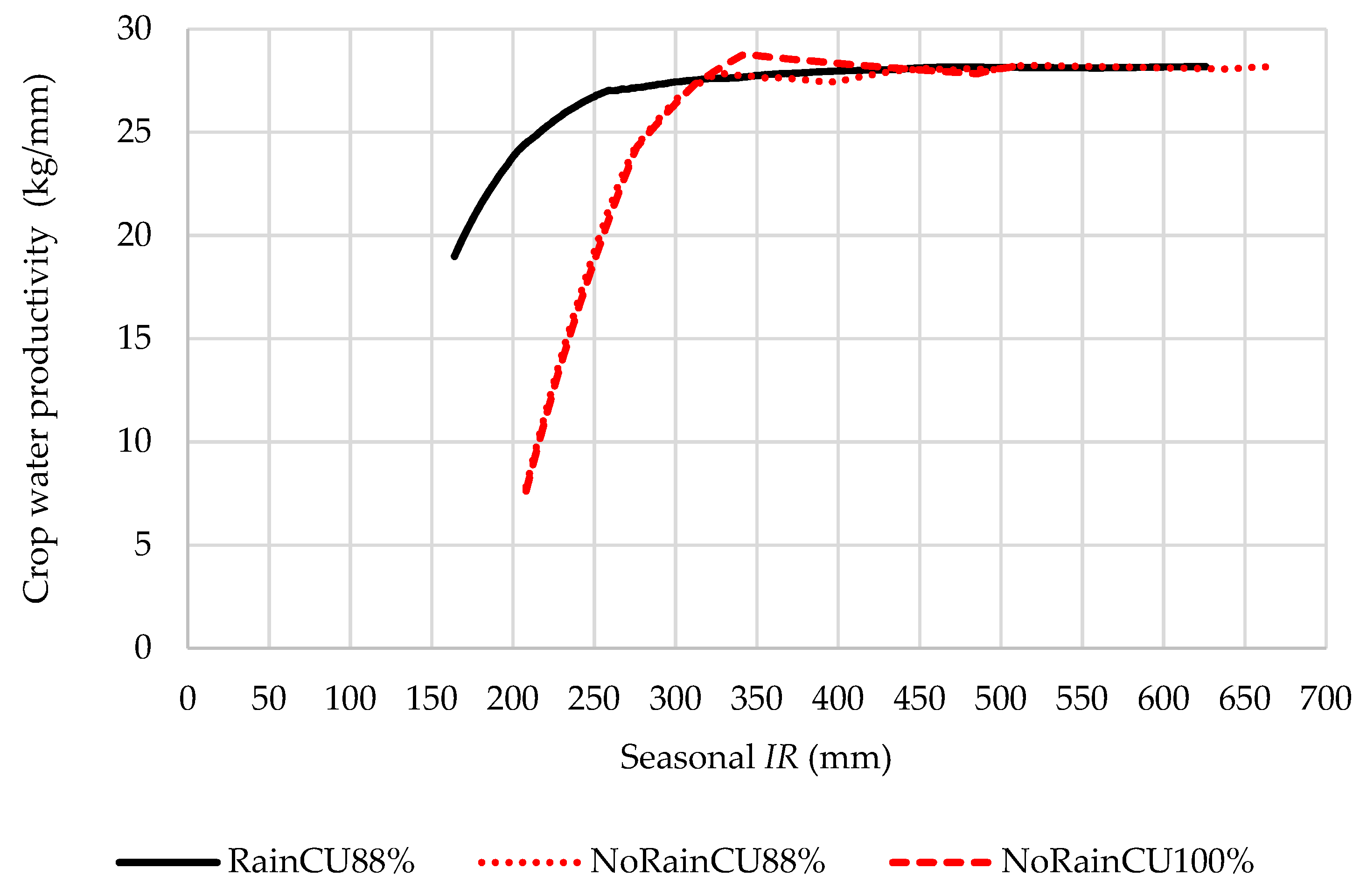
Irrigation farmers influence crop water use indirectly through applied irrigation water. Understanding water productivity in crop production therefore requires a thorough understanding of how irrigation applications influence crop water use. Figure 9 shows the relationship between applied irrigation water and crop water productivity for uniform and non-uniform irrigation applications while considering rainfall or not with a growth stage specific maximum $ETa$ deficit limit of 50%.

The results in Figure 9 show that CWP is, to a great extent, unaffected by applied irrigation water beyond applications of 317 mm irrespective of the scenario considered. For irrigation water applications greater than 440 mm, there is almost no difference between the scenarios, and the CWP of all the scenarios stabilizes around 28 kg/mm.

Considering the application of uniformity and non-uniformity while ignoring rainfall shows that the crop water productivity as a function of applied water is the same for both scenarios below 310 mm, which depicts the same relationship as AWP. However, it is evidenced that, between 330 and 440 mm, the uniformity scenario reaches a maximum of CWP at 28.7 kg/mm and slightly decreases to become constant at 28.1 kg/mm, while the non-uniformity scenario reaches a minimum at 27.4 kg/mm, and then also increases to be constant at 28.1 kg/mm. The non-uniformity scenario considering rainfall shows a consistent increase in CWP until it also becomes constant, as per the NoRain scenarios where the CWP shows a flat shape above 440 mm. Therefore, the above relationship confirms that if more water is applied, there is little or no change in CWP.

4.4. Rational Eeconomic Decision Making

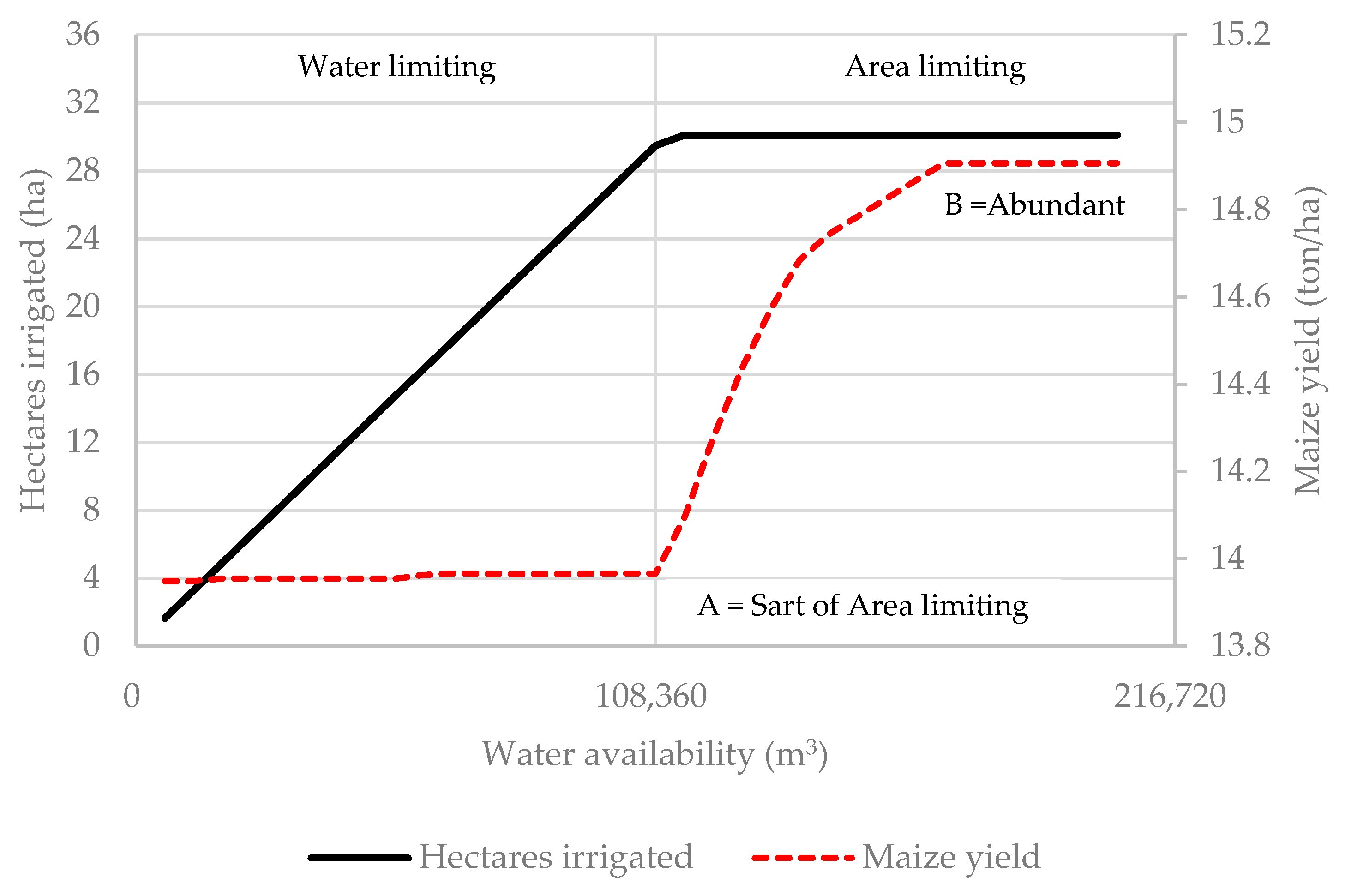
Cognizance should be taken of whether land or water is the most limiting factor of production when evaluating the economic rationality of agricultural water use. Figure 10 is used to define the water-limiting and area-limiting phases of production. When land is the most limiting production factor and water is abundant, a rational decision maker will apply irrigation water to the point where the value of the marginal product of applying the last incremental unit of water is equal to the cost of applying the additional water. Such a situation is depicted at point B. It is important to note that it is not economically justifiable to apply water to achieve a maximum crop yield of 15 ton/ha.

When water availability is reduced below point B, a rational decision maker will acknowledge the trade-off between increased profits from applying more water per hectare and the reduction in the total irrigated area necessary to allow higher application rates per hectare. For water availability between points A and B, it is profitable to reduce water applications per hectare with reduced crop yields while irrigating the total irrigation area. At some point, reducing water applications per hectare will become unprofitable and the only way to produce profitably is to reduce the area irrigated. Such a situation is depicted by water availabilities below point A where water is the most limiting production factor. The water-limiting case is characterized by a constant decrease in area irrigated to maintain profitable production levels per hectare.

Table 1. Economically optimized water use for the area-limiting and land-limiting cases for a uniform (CU100%) and non-uniform (CU88%) water application in the presence of rainfall (Rain) and no rainfall (NoRain).

	Unit	RainCU88%	NoRainCU88%	NoRainCU100%
Area-limiting case (Abundant water)
Margin above specified costs	R/ha	5236	5108	5423
Margin above specified costs	R/mm	9.36	7.65	10.68
Maize yield	ton/ha	14.91	14.99	14.99
Applied irrigation water	mm	559.67	668.11	507.79
Evapotranspiration	mm	530.25	532.28	532.28
Area irrigated	ha	30.10	30.10	30.10
Applied water productivity	kg/mm	26.63	22.45	29.54
Crop water productivity	kg/mm	28.11	28.18	28.18
Water-limiting case
Margin above specified costs	R/ha	4586	5012	5422
Margin above specified costs	R/mm	12.49	7.77	10.68
Maize yield	ton/ha	13.96	14.92	14.99
Applied irrigation water	mm	367.23	644.71	507.62
Evapotranspiration	mm	502.33	530.97	532.27
Area reduction	ha/6020 m3	1.64	0.93	1.19
Applied water productivity	kg/mm	38.01	23.14	29.55
Crop water productivity	kg/mm	27.79	28.10	28.18

shows the optimized results for the area-limiting case with abundant water and water-limiting cases when water applications are uniformly and non-uniformly applied while considering rainfall or not with a growth stage specific maximum $ETa$ deficit limit of 50%.

Next, these scenarios are discussed.

4.4.1. Area-Limiting Scenario with Abundant Water

Let us consider the effect of uniformity changes on the key output variables first while not considering the effect of rainfall. The optimized results show that the optimal water applications levels are very close to maximum yield application levels of 15 ton/ha for the two levels of uniformity. Consequently, the CWP values are both 28.18 kg/mm. The non-uniform application (CU88%) required 161 mm more water when compared to the 507 mm irrigation application of the uniform (CU100%) scenario. As a result, the AWP of scenario CU88% is only 22.45 kg/mm, which is 7.09 kg/mm less than the AWP of scenario CU100%. The higher AWP of scenario CU100% causes the margin above the specified costs per hectare and per millimeter for scenario CU100% to be the highest.

Rainfall increases the AWP from 22.45 to 26.63 kg/mm because the magnitude of deficit irrigation is larger when compared to scenario CU88% without rainfall. Increasing the level of deficit irrigation causes the soil to be drier, thereby increasing the probability that rainfall can be stored in the soil profile. Contrary to AWP increases, CWP is not affected to a large extent. Higher AWP causes the margins above specified costs per hectare and per millimeter to increase.

4.4.2. Water-Limiting Scenario

Results in Table 1 show that the area irrigated needs to be reduced by 1.19 and 0.93 ha per 6020 m³ reduction in water availability, respectively, for CU100% and CU88% scenarios to produce profitably at slightly increased levels of deficit irrigation when compared to the area-limiting case. Contrary to the no rain scenario, rainfall increases the level of deficit irrigation for the water-limiting case. Consequently, the margin above the specified costs per hectare is the lowest across all the scenarios. However, the margin above specified costs per millimeter of applied irrigation water is highest, which shows that under water-limiting conditions the profit margin for the scarce resource, water, is maximized. It should be noted that the overall profit for the rainfall scenario is still larger than the comparable no rain scenario, even though the margin above specified costs per hectare for the rain scenario is ZAR 426 /ha lower than the ZAR 5012 /ha of the no rain scenario. The reason for this is that the rain scenario applied only 367.23 mm of water compared to the 644.71 mm of the no rain scenario. By implication, 1.75 (644/367) times more area could be planted by considering rainfall compared to not considering rainfall in the model, which causes total profit generated with the same amount of water to be larger. The increase in the level of deficit irrigation associated with considering rainfall causes AWP to increase from 26.63 kg/mm under the area-limiting case to 38.01 kg/mm for the water-limiting case. Interestingly, CWP decreased slightly to 27.79 kg/mm.

5. Discussion

Many researchers have relied on mathematical programming models to provide guidance with respect to the allocation and use of irrigation water with the aim of increasing productive use. Modeling the soil–water–crop interactions necessary to determine the impact of irrigation scheduling on crop yield is complex and modelers need to make simplifications to overcome hardware and software limitations. Most often, these simplifications relate to the way researchers combine relative CWPFs with procedures to model inefficient water applications to derive the WPF and the assumptions regarding rainfall. When providing rainfall as a model input, the modeler implicitly assumes that rainfall is known with certainty and that irrigation schedules are optimized such that rainfall will result in no percolation. Inefficiencies are the direct result of technology choice and the timing and quantity of applied water in relation to the soil-water status. Modelers should carefully consider the assumptions made and their impact on results.

Results from this research show that the scope to increase CWP through reduced water applications is small for a rational decision maker with the objective of maximizing profit. The price ratio (irrigation cost/crop price) governing economic decision making is small in our case, indicating that decision makers will try to obtain near-maximum yields for both the area-limiting and water-limiting cases. Consequently, the portion of the WPF that is relevant for economic decision making and the corresponding portion on the CWPF is small, and therefore CWP does not change significantly. Considering rainfall increases the portion of the functions that are relevant for economic decision making. However, the portion remains small.

Contrary to researchers who argue that maximizing crop water productivity is useful in guiding decision making, this research concurs with researchers who argue in favor of using incremental benefits of applying irrigation water for decision making. The conclusion is that maximizing CWP or AWP will result in suboptimal economic outcomes when considering a specific technology set.