A Novel Surge Damping Method for Hydraulic Transients with Operating Pump Using an Optimized Valve Control Strategy

Abstract

Hydraulic transients may pose a critical threat to process operation due to devastating surge waves. This paper investigates hydraulic surge and damping control associated with pipe flow modeling and valve optimization. A one-dimensional transient model was developed using the modified instantaneous accelerations-based (IAB) model, considering energy dissipation, referred to as the compression–expansion effect, which was then solved by the Method of Characteristics (MOC). Analogous to solving valve operation by means of the traveling salesman problem (TSP), a novel surge damping strategy was proposed by applying an improved artificial fish swarm algorithm (AFSA). After validating the unsteady model and the optimization algorithm, wave surge damping effectiveness was evaluated on the basis of case studies in different pump running scenarios. The results showed that the proposed nonlinear optimized control method was able to reduce surge amplitude by 9.3% and 11.4% in pipe systems with and without running centrifugal pump, respectively, and was able to achieve a 34% time margin or a maximal 75.2% surge reduction in the case of using an positive displacement pump. The optimized nonlinear valve closure presents different shapes in fast closing and slow closing situations. The strategy proposed in the present study is beneficial for guiding valve real-time control, as well as providing a reference for valve design for the purpose of wave surge protection.

1. Introduction

During the process of fluid transportation through a pump, any rapid unexpected changes affecting fluid flow may cause the hydraulic transient phenomenon. In a water pipeline system, sudden valve closures or pump start-up/stoppage can generate such transient events, which are also known as a water hammer. Once the harmful pressure wave has propagated along the pipeline, there will always exist positive and negative pressure waves due to reflection. Hydraulic surge may cause severe damage to pipes or connected devices; on the other hand, the reflected negative waves associated with oscillating cavitation or water column separation can also affect the safe operation of the pump [1,2].

A water hammer is a type of pressure wave that propagates as a result of fluid oscillation at a corresponding degree. Such oscillation behavior is influenced by pipeline boundary conditions and the energy dissipation process, and accurate modeling of wave characteristics can be essential for pipe design and pipeline leakage or blockage detection [3]. Since pressure waves travel at a fast speed equivalent to that of the local speed of sound, safety precautions against wave surges and reflections are also regarded as an essential issue.

The accurate establishment of the unsteady friction model is important for modeling hydraulic surges in transient pipe flows, especially in the unsteady friction-dominated transient flow. With regard to the importance of unsteady friction, Duan et al. [4] found that unsteady friction makes a greater contribution in small-scale pipeline systems, where the timescale ratio of wave propagation to radial diffusion is low. Ghidaoui et al. [5] suggested that the quasi-steady and flow asymmetry assumptions may result in deviations in the wave shape over larger simulation timescales. Usually, convolution-based (CB) models and instantaneous acceleration-based (IAB) models are used in transient simulation. For the CB model proposed by Zielke, the Navier–Stokes equations of axial pipe flow are solved with the Laplace transformation, and the unsteady friction is described by the convolution of the past accelerations with different weighting functions [6]. Although it has the merits of a strong physical basis and less dependency on the determination of empirical coefficients, CB models commonly require great computational resources to deal with the local acceleration and weight function in the convolution integral across the full time range of all nodes. This results in limitations to the application of such models for long-distance pipelines stemming from their low-efficiency numerical calculations. To solve this challenge, Urbanowicz [7] developed a novel recursive formula for estimating the convolution integral weighting function, enabling more accurate and efficient calculation of unsteady wall shear stress. As the CB model was initially derived for laminar transient flow, Trikha [8] simplified the calculation method of the weight function by only calculating the convolution of the local acceleration and the weight function at the previous moment to obtain the result, thus extending the application scope of the CB model to transient turbulent flow. By distinguishing eddy viscosity variation in the outer and inner core regions, CB model founds extended application in smooth and rough pipelines with a two-region model [9], as well as further application in different flow regimes with a four-layer model [10]. However, the involvement of historical acceleration and the lack of a convection term makes the weighting-function-based model vulnerable to the accumulation of errors with strong convection, such as in low-frequency waves after rapid valve closure and high-frequency waves caused by a running pump [11].

The widely used IAB model considers unsteady friction on the basis of local and convective acceleration. Based on the Brunone model with one damping coefficient [12], Pezzinga [13] added a symbolic function to the convective acceleration term, making the modified Brunone model capable of describing both accelerating and decelerating flows. Considering the different roles of local acceleration and convection acceleration, Ramos et al. [14] proposed a two-coefficient model to better characterize the phase change and amplitude change in wave dissipation, requiring knowledge and experience to determine the empirical coefficients. Owing to the high computation efficiency and the convenience of its program implementation, the one-dimensional IAB-based model is more suitable for complex pipe systems involving large-scale calculations [15]. Nault and Karney [16] integrated an IAB unsteady model with compatibility expressions in order to simulate a pipe network, and a solver adaptive method was used to increase the computational efficiency. To increase the accuracy of the model for accumulated dissipation, a modified IAB model taking into consideration the compression–expansion effect of the fluid on energy dissipation was proposed by our previous work [17]. Further progress in model development can be found when integrating the 1-D model. For example, Wu et al. [18] studied the transient interaction between the pressure surge and the pump using a CFD coupling simulation; a similar trend in flow rates and pressure pulsation was achieved by joint simulation, with precise pressure results. He et al. [19] proposed a digital twin framework in the oil transportation process, where a control theory and data-driven method were integrated to improve the accuracy of the physical model. Despite the convenient application of the modified IAB model, it must be noted that difficulties still exist in modeling some transient situations, such as valve opening events or frequency-dependent friction flows [20].

One of the many applications for hydraulic modeling is in the evaluation of extreme transient events when using certain preventive measures. It is known that many factors can affect wave propagation and the amplitude of a hydraulic surge. Bettaieb et al. [21] investigated wave damping performance during pump failure events, and found that using viscoelastic pipes could be effective for attenuating wave fluctuation, due to their rheological properties, while attaching a flywheel to the pump motor reduced wave amplitude as well as extending pump shutdown time. Garg et al. [22] found combined configurations with glass fiber-reinforced plastic damped the celerity in the pipeline and improved the wave damping coefficient. Urbanowicz et al. [23] experimentally investigated the transient laminar flow of oil in small-diameter pipes; together with a novel numerical solution method, the impact of factors including fluid viscosity and pipe length on pressure fluctuation was effectively analyzed.

With regard to valve motion, Wan et al. [24] considered the putting off effect of the valve under pump runaway conditions, pointing out that if the valve closure happens too quickly, or at an unsuitable time, a more severe water hammer effect might be generated following pump failure. To reduce the water hammer pressure caused by pump trip, Wang et al. [25] investigated the effects of valve closing time on pump safety based on the pump runaway characteristics, and gave advice on valve selection for different lift systems. For pump startup, the adoption of damping torque slowed down valve closure and proved to be effective for eliminating the water hammer, compared to the high-speed startup condition [26]. For pump shutdown events, Triki and Essaidi [27] investigated the induced pressure wave behaviors in two-section piping systems in different materials. The LDPE-steel pipeline demonstrated the best performance in terms of achieving a lower pressure surge peak with an extended wave oscillation period.

Aside from the above-mentioned factors in pipe systems, Sattar et al. [28] estimated the effects of additional surge vessels on pumping mains experiencing pump failure, and applied an approximate solution on the basis of Monte Carlo simulation to simplify optimum sizing rather than using hydraulic calculation. Kubrak et al. [29] used thinner polymeric branched pipes to control water hammer in a steel pipeline, and observed that the pressure surge was successfully attenuated and that the damping effect was more obvious in the event of rapid valve closure. Mohammad Bostan et al. [30] introduced an effective shock damper in which an embedded spring chamber absorbs the compression wave and subsequently releases its energy when it encounters the expansion wave. By applying a short compound section as a damping component connected to the main pipeline, Triki and Trabelsi interestingly investigated effects of dual combination [31] and standalone inline or branching strategies [32] on water hammer control, finding that the HDPE-LDPE penstock-based branching strategy achieved satisfactory pressure wave damping performance, while the dual-design strategy was more beneficial than the standalone strategy.

Despite much effort and progress in the area of transient pipe flow and its corresponding preventive measures, most research has focused on the water hammer phenomenon caused by pump failure, where the associated surge prevention relies on structural changes to the pipeline system. The importance of surge damping during constant running of the pump prior to being disconnected cannot be neglected. Adding a protective device is not always an option in some pumping processes when aiming to minimize the water hammer generated by valve motion itself. Therefore, in this research, we investigate the flow transient effects for pumps during the running stage. Considering the advantages for both the estimation of transient flow containing high-frequency components and the optimization of calculation efficiency for large samples using the artificial intelligence method, the IAB-based model was applied with a modified dissipation model considering fluid compression and expansion. After treating the valve as a wave generator and investigating the closure problem by analogy with the traveling salesman problem, a preliminary exploration of valve closure optimization is performed making use of an improved swarm intelligence algorithm, and this is ultimately applied to achieve surge damping in different operating pump scenarios.

2. Simulation Model

2.1. One-Dimensional Unsteady Friction Model

To characterize the transient behavior of the pipe flow, the following assumptions are considered as a necessary simplification for the 1-D numerical model:

(1)

The liquid fluid complies with cross-section-averaged properties.

(2)

The water liquid is considered to be single phase without entrained air.

(3)

The pipe is elastic, and the fluid is compressible.

(4)

The pipe flow is assumed to be adiabatic flow.

One of the most distinct features of transient pipe flow is the frictional loss behavior associated with unsteady friction. As a widely applied method for representing such losses, a steady friction component is often overlaid with an unsteady friction component in transient models.

The steady friction loss is calculated as

$$J_s=\frac{fV\left|V\right|}{2gD}$$

(1)

where D is the pipe diameter, g is the gravitational acceleration, V is the flow velocity, and f is the Darcy–Weisbach friction factor, which can be calculated by the Colebrook–White equation.

The unsteady friction loss can be calculated using the one-coefficient IAB model [13],

$$J_u=\frac{k}{g}\left[\frac{\partial V}{\partial t}+sign\left(V\right)a\left|\frac{\partial V}{\partial x}\right|\right]$$

(2)

where k is the empirical coefficient, which can be determined empirically or by the trial-and-error method [33], $sign\left(V\right)$ is the signal of the instantaneous mean velocity, a is the wave speed, and$t$and x represent the temporal coordinate and axial space coordinate, respectively.

Since fluid compressibility has an obvious effect on pressure oscillation and wave propagation characteristics, the energy loss caused by unsteady friction considers the compression–expansion effect to model the subsequent wave dissipation more accurately.

The momentum equation along x-axis can be expressed as

$$\rho \frac{DV}{Dt}=-\frac{\partial p}{\partial x}+\frac{\partial }{\partial x}\left[\left(2\mu +{\mu }^{\prime }\right)\frac{\partial V}{\partial x}\right]+\mu \left(\frac{{\partial }^{2}V}{\partial y^2}+\frac{{\partial }^{2}V}{\partial z^2}\right)$$

(3)

where $\mu$ is the dynamic viscosity and ${\mu }^{\prime }$ is the second viscosity.

By expanding Equation (3) in a cylinder control volume with coordinate transformation and neglecting the small quantity term, the second viscosity term-related momentum equation can be obtained as follows:

$$\frac{1}{g}\frac{\partial V}{\partial t}+\frac{\partial H}{\partial x}+\frac{f{V}^2}{2gD}-\frac{{\mu }^{\prime }}{\rho g}\frac{{\partial }^{2}V}{\partial x^2}=0$$

(4)

With the introduction of the unsteady friction term caused by the compression–expansion effects, the modified unsteady friction loss expressing the energy dissipation term can be written as Equation (5), where the detailed derivation is given in [17]:

$$J_u=\frac{k}{g}\left[\frac{\partial V}{\partial t}+sign\left(V\right)a\left|\frac{\partial V}{\partial x}\right|\right]-\frac{k_d}{g}\left|\frac{{\partial }^{2}V}{\partial x^2}\right|$$

(5)

where k_d is the second viscosity coefficient that is relevant to Reynolds number, which can be determined using the trial-and-error method. With the incorporation of the modified unsteady friction term, the one-dimensional governing equations for unsteady flow can be obtained, which are known as the water hammer equations:

$$\frac{\partial H}{\partial t}+\frac{a^2}{g}\frac{\partial V}{\partial x}=0$$

(6)

$$\frac{\partial H}{\partial x}+\frac{1}{g}\frac{\partial V}{\partial t}+\frac{fV\left|V\right|}{2gD}+J_u=0$$

(7)

These equations characterize the transient pipe flow behaviors, and contain two unknown variables: piezometric head H and flow velocity V. The hyperbolic partial differential equations are solved by the method of characteristics (MOC) in this study.

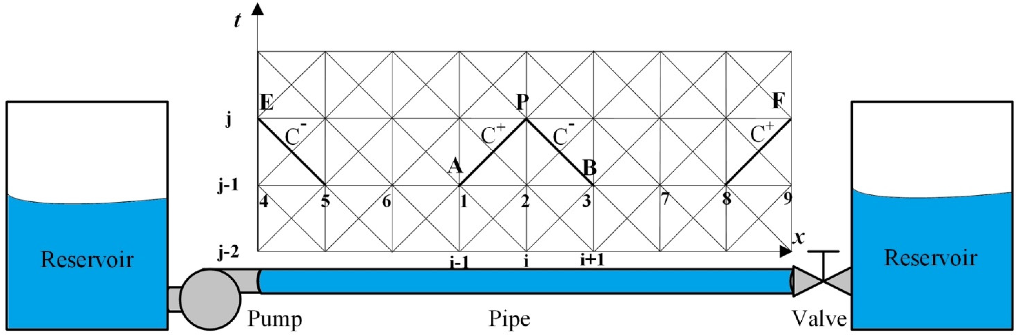
2.2. Physical Model and Solution Method

Figure 1 shows the investigated hydraulic system, in which a pump connected to an upstream reservoir is used to transport water fluid downstream through a horizontal pipeline. A valve positioned downstream is often used to regulate or control the transportation process, and its shutdown behavior directly affects the generated hydraulic phenomenon. To study hydraulic transient behavior and valve optimization strategy,

Table 1. Parameters for test cases.

Parameters (Unit)	Values
Initial tank head, Hres (m)	128
Initial flow velocity, V0 (m/s)	0.94
Pipeline length, L (m) Wave speed, a (m/s)	98.11 1298.4
Pump rotational speed, npump (r/min) Pump designed head, Hpump (m) Pump designed velocity, Vpump (m/s)	8000 165.9 0.88
blade numbers	8
Valve closing time, tc (s)	0.1~0.5
$\mathrm{Water} \mathrm{density}, \rho$ (kg/m3)	997.59
$\mathrm{Dynamic} \mathrm{viscosity}, \mu$$(\mathrm{Pa}·\mathrm{s}$)	0.947 × 10−3
empirical coefficient k second viscosity coefficient kd Darcy–Weisbach friction factor, f	0.0138 20.258 0.0224

lists the key parameters of a typical reservoir–pump–valve system for the purpose of our case studies. The initial head and flow rates are set for the reservoir without pump operation, while the head and flow rate comply with the pump characteristics curve in the pump cases.

As shown in Figure 1, the MOC discretization method is applied as a numerical solution scheme using rectangular grids. In this way, the ordinary differential equation (ODE) transformation of the hydraulic transient model needs to constitute a grid system, where time and space derivatives are discretized along the vertical and horizontal axes. By dividing the pipe into uniform segments with a length of$\mathsf{\Delta }x$, the time step for the pressure wave to propagate in each segment is $\mathsf{\Delta }t,$which is equal to$\mathsf{\Delta }x/a$. It is assumed in all simulation cases that the water flow originates from a reservoir with infinite volume, and the short draft tube between the pump and the reservoir is neglected in the analysis.

For the interior node P, the transformed ODE for positive and negative characteristics C⁺ and C⁻ can be expressed as

$$H_P=C_P-B{Q}_P$$

(8)

$$H_P=C_N+B{Q}_P$$

(9)

where

$$C_P=H_A+B{Q}_A-R{Q}_A\left|Q_A\right|-\Delta x{\left(J_u\right)}^{+}$$

(10)

$$C_N=H_B-B{Q}_B+R{Q}_B\left|Q_B\right|+\Delta x{\left(J_u\right)}^{-}$$

(11)

$$B=\frac{a}{gA}$$

(12)

$$R=\frac{f\Delta x}{2gD{A}^2}$$

(13)

The simultaneous Equations (10) and (11) can be used to solve the unknown quantity at P on the basis of the known quantities at points A and B.

For a frequency centrifugal pump located at the pipe’s upstream, its operating characteristics can be described by the performance curve when the motor-driven impeller runs at a constant speed. The head for the boundary condition is modeled as follows:

$$H_E=H_S+Q_E\left(a_1+a_2{Q}_E\right)$$

(14)

The above equation provides the upstream pump boundary conditions with a known H-Q performance curve, which typically shows a monotonically decreasing trend between the head and the flow rate. In this study, the performance curve of the centrifugal pump was produced using test data from [34], where the shut-off head H_S was 165.92, the coefficient constant a₁ was 7.07, and a₂ was −1.09.

By solving Equation (14) with the negative characteristic line C⁻, the flow rate $Q_E$can be obtained as follows

$$Q_E=\frac{1}{2a_2}\left[B-a_1-\sqrt{{\left(B-a_1\right)}^2+4a_2\left(C_N-H_S\right)}\right]$$

(15)

Since there is limited information available for the transient-state turbine characteristics, the pump transient-state characteristics can be obtained on the basis of the steady-state performance curve, which appears to be a valid assumption for most typical engineering applications [35].

As a result of the blade–tongue interaction of the pump, the instantaneous pressure and other flow parameters varied with time [36,37].

By imposing a 10% pressure fluctuation range on the pump characteristics [38], the outlet pressure can be regarded as a superposition of the steady-state pressure and the pulsating component, as follows:

$$H_E^{\text{'}}=H_E+0.1H_E·\sin \left(wt\right)$$

(16)

This simplified model implementation better characterizes the pulsating nature of the pump outlet signal, while keeping the time-averaged performance curve unchanged.

For a positive displacement pump located at the pipe’s upstream, the flow rate is set as a constant known parameter, and the pump head is calculated by integrating the instantaneous flow rate with the negative characteristic line C⁻, which is the reversal of the centrifugal pump case.

The relationship between flow rate and the hydraulic head of the downstream valve can be determined according to the orifice outflow law, as follows:

$$\frac{Q_F}{Q_0}=\frac{C_d{A}_G}{{(C_d{A}_G)}_0}\sqrt{\frac{H_F}{H_0}}={\tau }_V\sqrt{\frac{H_F}{H_0}}$$

(17)

where Q_F and Q₀ are the transient and steady flow rate through the valve, respectively, and H_F and H₀ are the hydraulic head in the transient and steady state, respectively.

The common relationship between the valve opening ${\tau }_V$ and the closing time can be expressed as:

$${\tau }_V=1-\left(\frac{t}{t_c}\right)$$

(18)

For the whole pipeline system, when the initial values and boundary conditions are all set, the discretized scheme is further assigned for the discretization of the partial differential term in the governing equations. In the one-coefficient IAB unsteady friction model, the convective acceleration and local acceleration terms can be discretized along the positive characteristic equation C⁺, in opposition to C⁻, as follows:

$$\left\{\begin{array}{c}\frac{\partial V_{i,j}}{\partial x}=\frac{V_{i,j-1}-V_{i-1,j-1}}{\Delta x}\\ \frac{\partial V_{i,j}}{\partial t}=\frac{V_{i,j-1}-V_{i-1,j-2}}{\Delta t}\end{array}\right.$$

(19)

In the modified unsteady friction term considering the compression–expansion effect, the diffusion term can be discretized using the nearest three adjacent points:

$${\left(\frac{{\partial }^{2}V}{\partial x^2}\right)}_P=\frac{V_{i-1}^{j-1}-2V_i^{j-1}+V_{i+1}^{j-1}}{{\left(\Delta x\right)}^2}$$

(20)

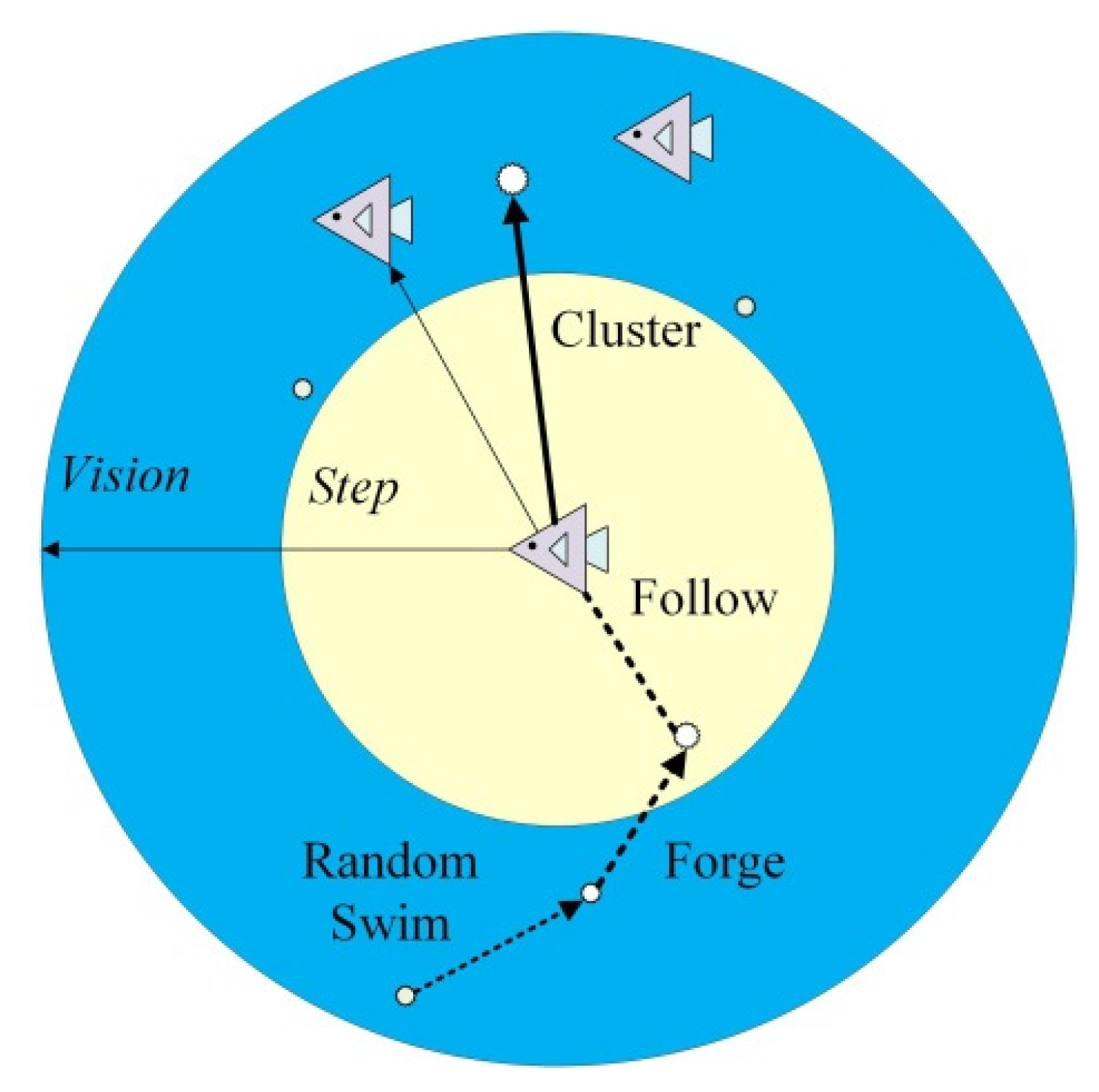
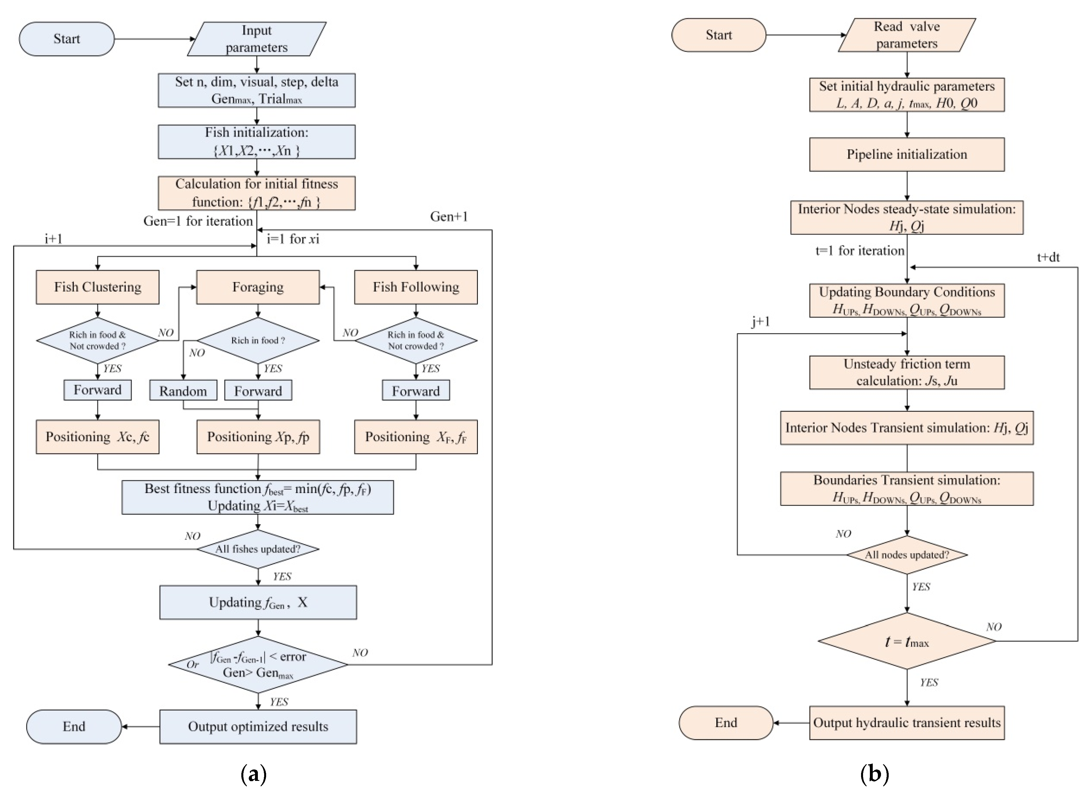
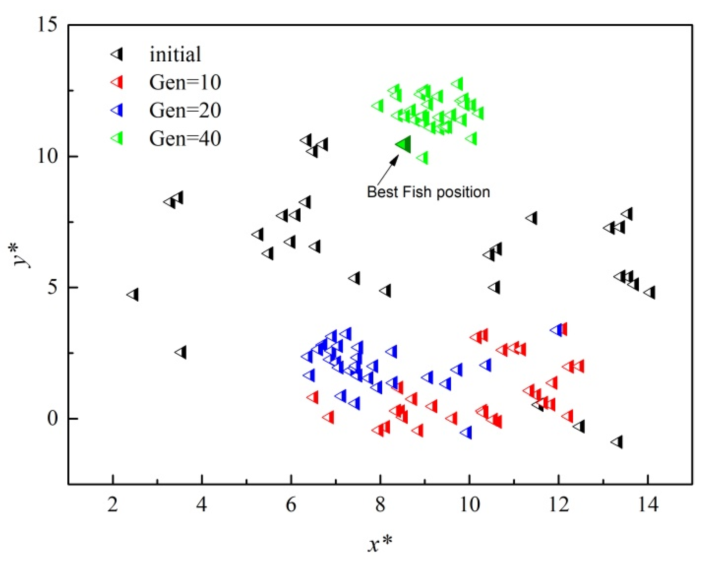
3. Optimization Scheme Using ASFA

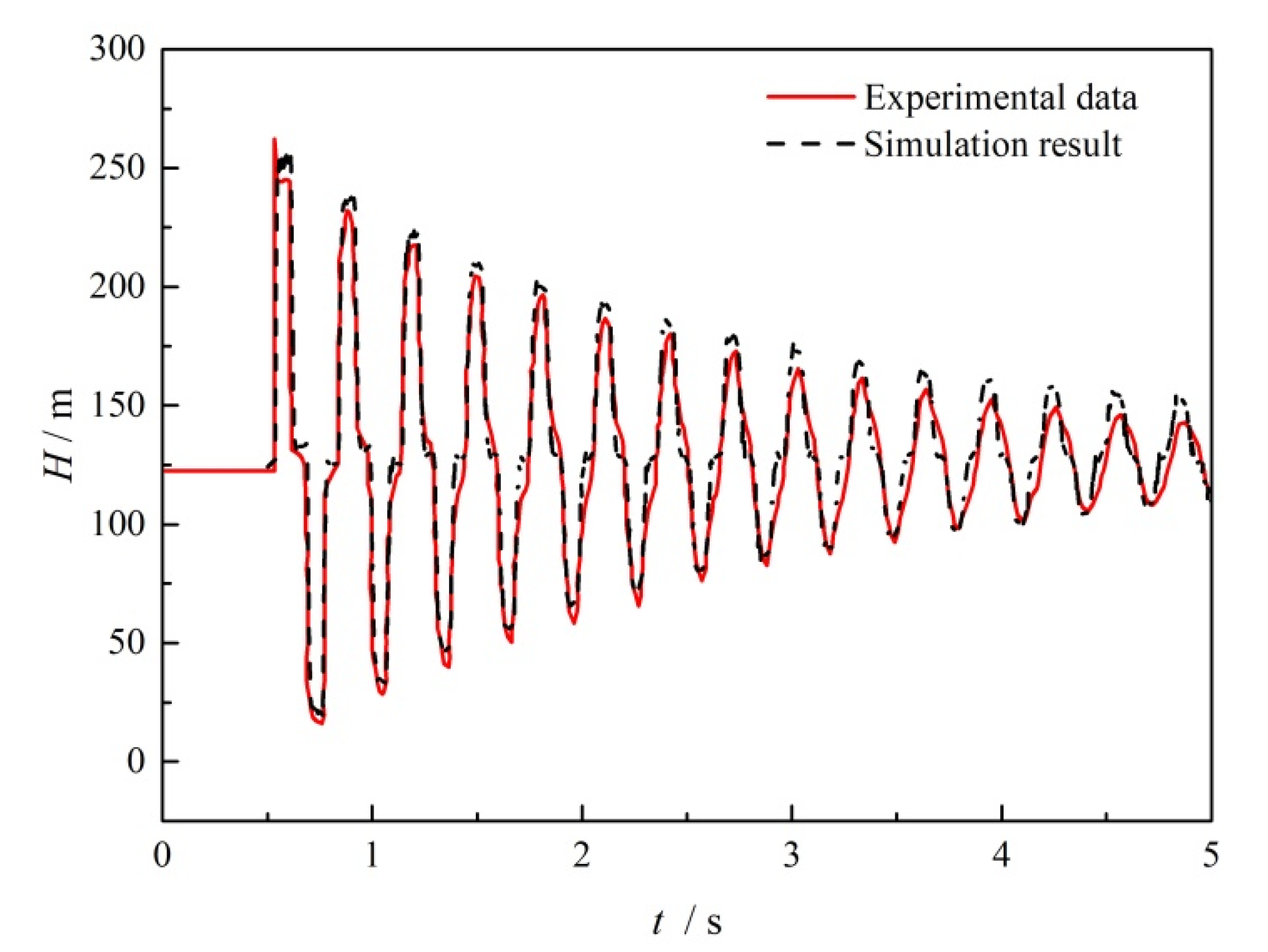
The problem being investigated is the pressure surge transmitted in the hydraulic pipeline caused by the valve’s sudden closure. The aim here is to design a valve shut-off procedure with a prescribed closure time that is able to minimize the pressure surge value, which can be regarded as having a negative impact on pipe system safety. By analogy, this valve motion can interestingly be converted into a traveling salesman problem (TSP). Different valve openings are regarded as serial locations that need to be visited by a salesman in accordance with a scheduled time sequence.

As can be seen in Figure 2, in a fixed total amount of valve closing time, the starting location is the place at which the valve opening is equal to 1.0, after valve operations, the finishing location is the full closure point, with an opening value equal to 0. In this problem, traditional valve motion (black line) can be seen as a linear visiting arrangement, which means an equivalent amount of time is spent during the sequential valve motion. This study preliminarily proposes nonlinear valve opening procedures (blue line). Different traveling times are assigned to different valve opening locations, and the visiting sequence is no longer required to maintain the same direction all the time. Then, the problem becomes a search for a time interval arrangement during valve closure that is able to minimize the pressure surge in the hydraulic pipe system. It is noted that the 10 valve opening points were selected in this study in order to present a preliminary demonstration; more or fewer intermediate points can be selected, depending on different amounts of available computational power.

Biotic populations in nature behave with a high degree of wisdom and logic. The ASFA is a novel swarm intelligence algorithm proposed by Li et al. [39]. As a bionic random search optimization algorithm, it has distinct advantages in solving nonlinear and discrete optimization problems due to its parallel global tracking features. With the help of this optimization algorithm, the requested time for different valve openings can be obtained.

Figure 3 shows the optimization process using artificial fish. Each fish X simulates ecological fish behavior when carrying variable amounts of information and swimming towards optimized value iterations, such as a fish’s instinctive response to the local environment. When the artificial fish finds a position with better food density within its field of vision, it moves in that direction by a certain step. During repeated searching, moving and comparing new locations with the current food density state and crowdedness threshold, one member of the swarm will finally arrive at the best position, thus optimizing the target function. The two conceptual parameters mentioned, vision and step, determine the movement behavior of the artificial fish in the search for an acceptable result.

Although ASFA is an effective swarm intelligence algorithm, it still has drawbacks, including slow convergence rate and convergence with local optima. In this study, stochastic behavior is added to enhance the possibility of escaping from local optima. Fish clustering and fish following are also integrated to increase the convergence speed of the fish swarm. The following equations describe each key principle of the applied algorithm.

The fish swarm is a natural behavior of fish during movement for to the purpose of foraging together and avoiding the enemy; when the food density (fitness function) in the center position X_V of all visible fish is better than that at the current position Xi while also satisfying the crowdedness standard, it steps forward to the swarm center and reaches a new position X_c,

$$X_c=Xi+\left(\frac{X_V-Xi}{\parallel X_V-Xi\parallel }\right)·ste{p}_{rand}$$

(21)

Otherwise, artificial fish execute the prey behavior, which is a biological instinct that tends to be used when food exists in higher concentrations:

$$X_s=Xi+Visio{n}_{rand}$$

(22)

where $X_s$ represents repeated random searching positions within the fish’s field of vision. Then, the fish moves forward to a new position X_p:

$$X_p=Xi+\left(\frac{X_s-Xi}{\parallel X_s-Xi\parallel }\right)·ste{p}_{rand}$$

(23)

It is noted that large fish fields of vision and step sizes improve the algorithm’s global search capability, while small values benefit the algorithm’s local search capability.

To further enhance the convergence speed, fish following behavior is added to simulate natural behavior whereby neighboring fish tend to quickly swim to the best position $X_F$if one of them $X_j$finds food:

$$X_F=Xi+\left(\frac{X_j-Xi}{\parallel X_j-Xi\parallel }\right)·ste{p}_{rand}$$

(24)

Another behavior is added to further avoid becoming trapped in local optima, in the form of a random swim to a new position $X_{t+1}$ to find new food or fish crowds:

$$X_{t+1}=X_t+ste{p}_{rand}$$

(25)

The main key parameters for implementing the above algorithm are given in

Table 2. Parameters for the optimization algorithm.

Parameters	Description	Values
Vision	visual radius	0.1
step	moving distance	0.01
n	artificial fish quatities	30
dim	artificial fish dimension	10
delta Trailmax Genmax	fish swarm crowdness maximum trial number maximum iteration number	27 30 500
error	convergence error	1 × 10−4

. These parameters remain constant until final convergence. Like most artificial intelligence algorithms, the selection of these values depends on practical experience and achieving a balance between computational resources and accuracy. In this study, a rigorous criterion was set for convergence, whereby the error between updated values of the fitness function (pressure head) and the averaged value among last 10 results must be less than 1 × 10⁻⁴.

The calculation procedure is given in Figure 4. For the main optimization loop I shown in Figure 4a, firstly, input data and ASFA initial settings are given, and parameters include fish dimension, population size, vision and step sizes, crowding factor δ, and number of trial iterations. Secondly, a group of random fish is generated with initial positions, and then the hydraulic analysis in loop II is carried out to obtain the adaptive values, and the best values are recorded on the bulletin board. Thirdly, the behavior of each individual fish performing selective behaviors, which include fish clustering, fish following, foraging and potential stochastic swim, is evaluated and determined. Fourthly, after determining artificial fish behavior, their position is updated as X_c, X_p, and X_F. If an individual fish position is superior, then the bulletin board is updated with the position of the optimal fish. This evaluation continues until evaluation for all fish has been completed. Finally, when the termination criteria are satisfied by means of an acceptable error or the iteration limit being reached, the algorithm ends with the optimized results being output.

All orange frames in Figure 4a involve the sub-loop of hydraulic transient calculation, the procedures for which are given in Figure 4b. Firstly, together with the given hydraulic parameters, the valve motion parameters, termed as fish position, generated by ASFA are read. Secondly, the pipeline is initialized using the steady-state calculation for the first time step. Thirdly, the boundary conditions are updated, and the unsteady flow model is solved using the MOC method to obtain all node information, including head H and flow rate Q. Finally, node hydraulic information is obtained, as calculation time reaches its maximum value.

4. Model Validation

A classical reservoir–pipe–valve system is first used to validate the unsteady hydraulic model used in this study. The simulation settings were set in accordance with the experiment described in Ref. [40]. The configuration is similar to that described in the schematic diagram in this study, except that the pump device has been removed. Along the pipeline, the number of grid nodes is set to 100, so that the grid space and step time satisfy the Courant–Friedrichs–Lewy condition with adequate precision.

The simulation results using the modified IAB-CE model are compared to the experimental data in Figure 5. In this test case, the pressure surge is monitored at the mid-point of the pipe after a rapid valve closure. It can be seen that both the pressure surge amplitude and the waveform in the simulation results are in good agreement with the experimental data at the pipe’s midpoint. The applied numerical scheme considers unsteady friction, including the compression–expansion effect, providing relative calculation errors for the pressure surge within 2.16%. The satisfactory consistency, especially in the subsequent wave fluctuation, guarantees the accuracy of target function for performing optimization on the basis of the present hydraulic model.

For the modified ASFA optimization method implemented in this study, its validity was also tested with representative benchmark functions, and the results are presented in Figure 6. The first test function was the sphere function $f1\left(x\right)={{\displaystyle \sum }}_{i=1}^D{x}_i$ in the searching range [−100, 100]^D=30. With an acceptance of 0.01, the minimum value 0 was obtained at (0, 0) for this function. The second test function was $f2\left(x\right)={{\displaystyle \sum }}_{i=1}^{D}100{(x_{i+1}-x_i{}^2)}^2+{(x_i-1)}^2,$ which is also a unimodal function, and is known as the Rosenbrock function. In the searching range of [−10, 10]^D=30, the minimum value 0 was found at (1, 1) with an acceptance of 100 [41]. As can be seen, the minimum values obtained from the presented optimization method were 1.89 × 10⁻⁶ in Figure 6a and 3.17 × 10⁻⁵ in Figure 6b, respectively.

In Figure 6c, Schwefel’s optimization problem was selected. It is known that this multimodal function is a typical deception problem, where the global minimum value 0 is hidden in a valley at (420.97, 420.97), far from other local optimal valleys. Hence, it is difficult for the algorithm to jump out of local optimal points, which it easily falls into. When testing the transformed function$f3\left(x\right)=418.9829D-{{\displaystyle \sum }}_{i=1}^D{x}_i\sin \sqrt{\left|x_i\right|}$, the optimization results showed the successful location of the valley compared with the theoretical values, validating the performance of the proposed ASFA as well as its feasibility for optimizing the nonlinear problems in this study.

5. Results

For a fixed valve closing time, as is required in order to achieve quick responses to hydraulic events, it is important to know the flow behavior during flow transients. Different arranged time lengths and pump types have different effects on the pressure surge generated by valve closure. With the help of the developed IAB-CE model and the modified ASFA optimization method, the characteristics of pressure propagation and the corresponding wave damping method are analyzed.

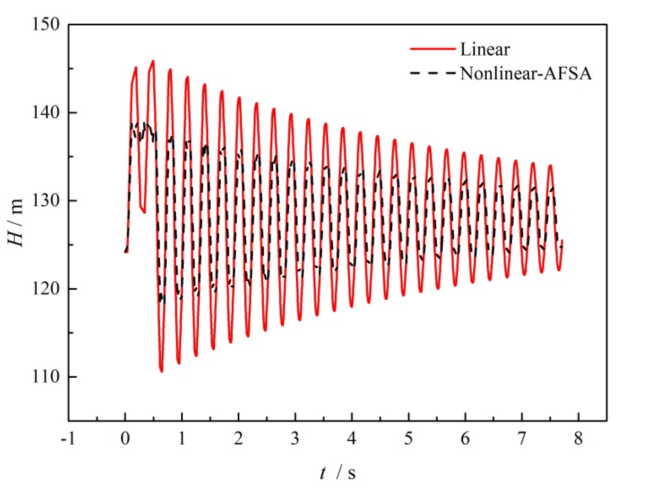
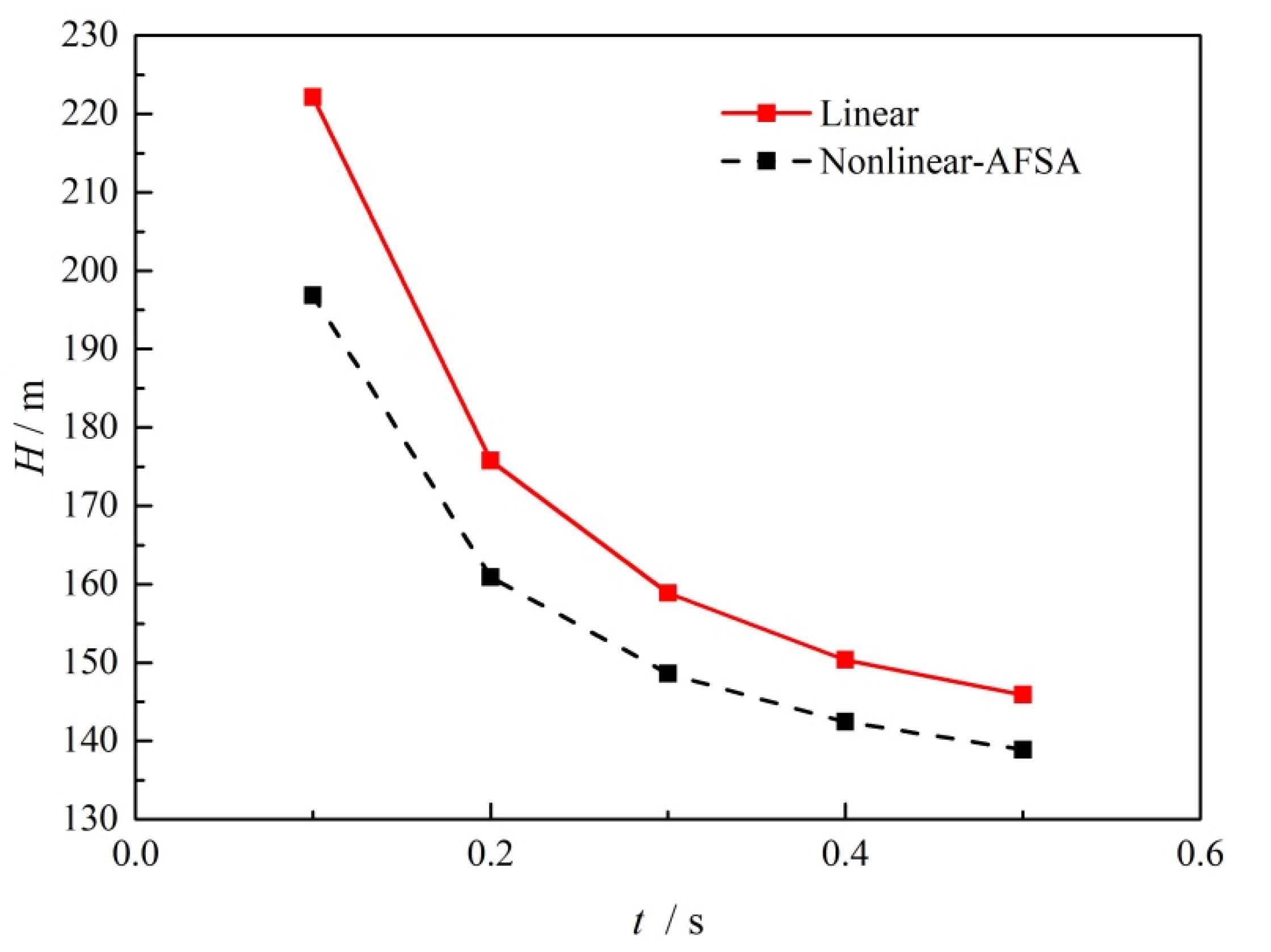
5.1. Wave Damping Case without Pump Operation

In this case, there is no pump operation, and the associated pump loss is neglected. Pipe flow becomes unsteady after valve closure, and the generated pressure wave propagates to the upstream reservoir, with a pressure surge being recorded in the pipeline.

To visualize the optimization process, Figure 7 and Figure 8 serve as an example in this work, which is similar in other cases. It can be seen in Figure 7 that the initial 30 artificial fish in black triangles representing the valve opening sequences are initialized in random positions. After the implementation of the ASFA optimization process, the fish start to cluster and follow the optimal fish at the time, escaping from local optimum positions by foraging throughout the search space. At the 40th generation of the swarm of fish, the leading fish depicted with green triangles emerge at the best position, and the searching process is then terminated.

Figure 8 shows the variation in the fitness function and convergence curve with increasing numbers of iterations. The black line represents the fitness function as the optimal pressure head value, while the blue line represents the convergence curve. It can be seen that the optimal head value fluctuates during the initial clustering swarm at around five iteration steps, and soon the head value quickly decreases with the rapidly decreasing convergence curve. After 10 iterations, the minimization of the optimized head value tends to slow down, and it almost remains unchanged after 40 iterations, while the convergence curve decreases to an extremely low level.

On the basis of the obtained optimized valve closure time arrangement, Figure 9 compares the transient pressure head at the midpoint of the pipe when the valve is closed within a time of 0.1 s. As can be seen from this figure, the solid red line is the result when performing linear valve closure, while the dashed black line is the results when using the optimized nonlinear valve closure. Compared to the shark waveform observed for linear closure, the wave peaks are split into double peaks, and the amplitude is obviously reduced, along with the wave valley, for the same lengths of valve closing time. The results suggest that with the optimized valve operation, the hydraulic pressure fluctuation can be damped in both directions without changing the wave frequency. The safety risk can then be reduced by avoiding larger over pressure and negative pressure.

It is known that extending the valve closing time contributes to weakening the water hammer phenomenon. Figure 10 shows the pressure fluctuation when valve closing time is extended to 0.5 s. As can be seen from this figure, with the gradual reduction in valve opening time, there is a corresponding increase in the pressure at the midpoint, which then falls coupled with the upward reflected negative wave. After the full closure of the valve, the maximum and minimum pressures are obtained, and afterwards the damped oscillation can be observed in the pressure waveform due to continuous frictional loss. For the case of optimized valve operation, it can be observed that the degree of pressure fluctuation can also be decreased by using a longer valve closing time.

To investigates the pressure surge damping performances by the optimized nonlinear valve closure, the effect on the pressure surge amplitude is compared for various valve closing times. In each case, for the given closure times, the optimization using ASFA is carried out to generate a time sequence for optimized valve operation. As can be seen in Figure 11, the pressure surge amplitude caused by valve closure decreases with increasing valve closing time, and the descending slope also becomes more shallow with increasing valve closing time. However, for the designed nonlinear closure case, the pressure surge amplitude decreases of 11.4%, 8.5%, 6.5%, 5.2%, and 4.8%, respectively, compared to normal valve operation in 0.1 s to 0.5 s, can be achieved.

The optimized valve operation characteristics are shown in Figure 12. The x axis represents normalized time by dividing the total closing time. It can be clearly seen that the operation with a closing time of 0.1 s has the largest deviation from linear operation, indicated by the diagonal dashed line. This can be explained by the working characteristics of the valve, as it plays the role of a pressure wave generator by adjusting the different valve openings for different time periods. Within a very limited amount of time, the downstream valve needs to generate a greater expansion wave in order to reduce the superimposed wave energy at the pipe’s midpoint. At around 0.014 s, 0.028 s, and 0.092 s, the valve opening becomes larger in order to generate a subsequent negative pressure wave travelling upwards, so that the pressure surge can be damped, coupled with the following compression wave. It should be noted that the valve opening curve can either be applied in precise valve operation by means of real-time control or used as a structural guideline for providing corresponding flow resistance in valve design for specified damping problems.

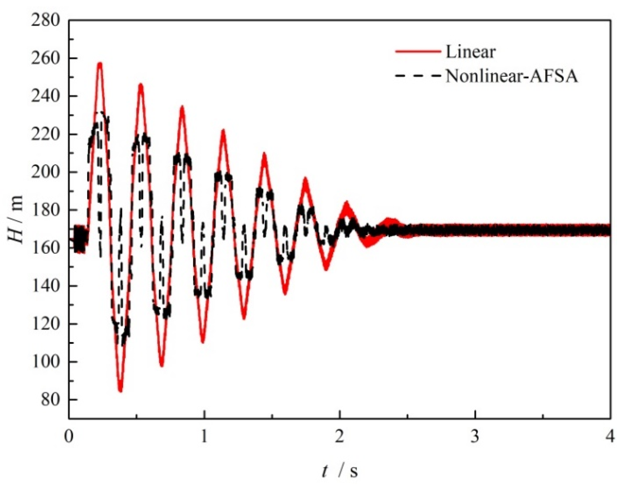
5.2. Wave Damping Case with Centrifugal Pump Operation

In some transient events such as pump failure or sudden stoppage, four quadrants and eight zones of possible pump operation can be classified on the basis of the direction of flow, pressure, rotation and torque [42]; a complete head and torque characteristic curve is used to describe the pump characteristics, including reverse running state [43]. When a pipeline connected to a centrifugal pump undergoes unexpected valve closure, a hydraulic transient occurs even when the pump is still being motor-driven at the same rotation speed without powering off. As shown in Figure 13, the pressure head at pipe’s midpoint also fluctuates following the peak and valley values after full closure of valve at 0.1 s. In comparison, the optimized nonlinear closure also reduces the pressure surge amplitude with a split waveform, appearing to enter steady oscillation slightly earlier due to the decreased pressure surge during the initial transient stage. It needs to mentioned that although the pressure can be temporally controlled to within an acceptable range following valve closure, it is still necessary to shut off the motor as early as possible in order to avoid overheating of the water, since the flow circulation is no longer activated while the impeller is still rotating at a high speed.

For valve closure over a larger time length of 0.5 s, a comparison of the pressure fluctuation results is presented in Figure 14. It can be observed that, after the valve is fully closed after 0.5 s, the recorded wave peak–wave valley amplitudes decrease from 186.8 m–155.6 m, to 179.8 m–161.7 m. Additionally, due to the timely adjustment of the nonlinear valve opening throughout the whole valve motion period, the first wave peak of 186.3 m—wave valley of 162.6 m was also reduced to 179.7 m–172.1 m, compared with linear valve operation. Since the entrained energy of the fluid is gradually released for water hammer events with slow valve closure, the surge is relatively low compared to valve closure in 0.1 s, and the fluctuation only lasts for 1.02 s, before emerging into pump output oscillation caused by blade sweeps.

Figure 15 shows the pressure surge damping performance with centrifugal pump operation. It can be seen that the variation trend is similar to that in the case described in Figure 11. Furthermore, in comparison with normal linear valve operation, the pressure surge amplitude with the optimized nonlinear valve closure exhibited decreases of 9.3%, 6.4%, 5.3%, 4.2% and 3.8%, respectively, as well. This suggests that the developed nonlinear closure method using ASFA could also be suitable for damping the pressure surge in cases when the pressure input is not steady and varies with time. Any safety margin also in return limits the selection of the pump and connected devices.

To investigate the optimized valve operation characteristics with the centrifugal pump, Figure 16 shows the variation in nonlinear valve opening with normalized time. As can be seen, for a short operation with a closing time of 0.1 s, the valve opening curve has the largest deviation from the linear operation curve. It rises at 0.0008 s, 0.0659 s, and 0.087 s during operation, while an expanding wave is generated by the valve opening. The overall characteristic curve is similar to an “И” shape, where the valve opening tends to decrease rapidly at first, before becoming smooth, followed by a rapid subsequent increase. Like all other cases with a longer valve closing time, the valve opening results in a rapid reduction during the last stage. Although wave propagation and superposition are complicated when considering variable valve motion together with the changes in pipe flow unsteady frictional loss, the control strategy using ASFA presented as a conceptual demonstration can serve to provide design guidance, and is expected to also be feasible in complicated pipe system optimization problems.

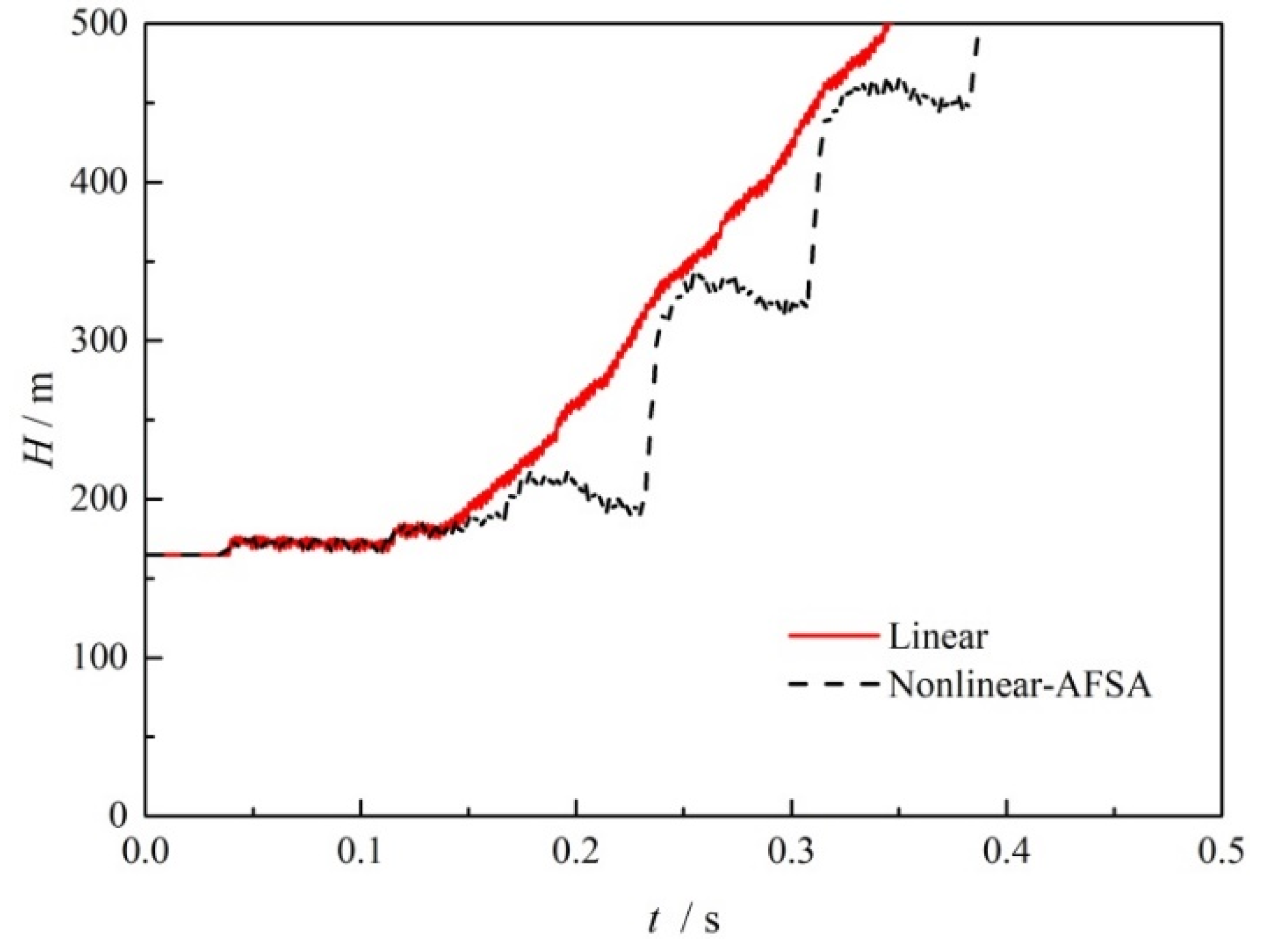
5.3. Wave Damping Case with Positive Displacement Pump Operation

Another case to consider is that of a pipe transferring fluid through a displacement pump. One major difference is that the displacement pump faces a severe pressure rise over a short time after choking, which is also known as pressure buildup. This rapid increase in pressure can easily exceed the upper limit of pipe safety, or cause damage to connected devices, including the pump itself.

By setting 500 m as the assumed head limit for the pipe, Figure 17 shows the protective effects of the optimized nonlinear valve closure on surge damping. It can be seen that the pressure rise becomes obvious following full valve closure. For the linear operation case, the midpoint pressure increases proportionally with pumping time, while for the optimized situation, the waveform is distorted and the pressure increase with time exhibits fluctuations. Although the rise in the pressure head is unavoidable for the positive displacement pump, and eventually increases to 500 m, it can be observed that the pressure in the optimized case remains constantly lower than in the linear closure case. Moreover, it takes 0.39 s to reach the head limit of 500 m, compared to 0.34 s for the traditional closure case without nonlinear control. This 14.7% extension of reaction time means that there is more time for a precise hydraulic system to be able to disconnect the pumping system.

In Figure 18, it can be seen that there was a more obvious improvement in surge damping when using the optimized nonlinear closure with a longer closing time of 0.5 s. It can be seen the distance between the two curves is larger, and the times required for the traditional and optimized operation cases to reach the pipe head limit are 0.53 s and 0.71 s, respectively. An additional 34% of extra time can be used to take precautions against the surge limit in the pipe system.

Figure 19 shows the results of the calculated head at the midpoint 1 s after full valve closure over different times. It can be seen that for the traditional linear valve operation, the size of the resulting pressure head rise increases linearly from 349.8 m to 693.1 m with increasing valve closing time from 0.1 s to 0.5 s. This is mainly because the built-up pressure accumulates when subjected to a longer compression time. However, with the optimized nonlinear valve operation, the amplitude of the resulting pressure rise is greatly reduced, from 336.5 m to 395.7 m, with a maximum reduction of 75.2% in head surge being recorded after full valve closure. Therefore, it is suggested that even for the positive displacement pumping process, beneficial consequences can still be expected from surge damping by applying the optimized nonlinear valve control method based on ASAF method in hydraulic transient events.

The optimized valve operation characteristic curves with the positive displacement pump are presented in Figure 20. As can be seen, all curves are above the diagonal line in terms of their variation with normalized time. This means that the valve prefers a slow switch-off or an even switch-on in the beginning. Except for the 0.1 s closure case, all valve opening curves exhibited a relatively smooth variation during the initial valve operation stage, before rapidly decreasing to the fully closed state. A similar “И” shape was also found for the 0.1 s closure case, indicating that larger valve motion amplitude is required to diminish the wave surge in a limited period of time.

6. Conclusions

In this study, a one-dimensional hydraulic model considering compression–expansion dissipation was implemented to describe transient flow; combined with improved AFSA optimization, surge protection for pipes with different operating pumps was evaluated. The following conclusions were drawn:

(1)

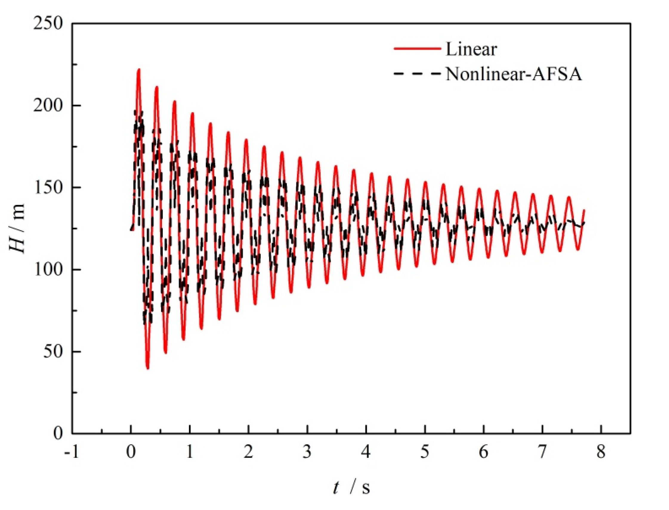
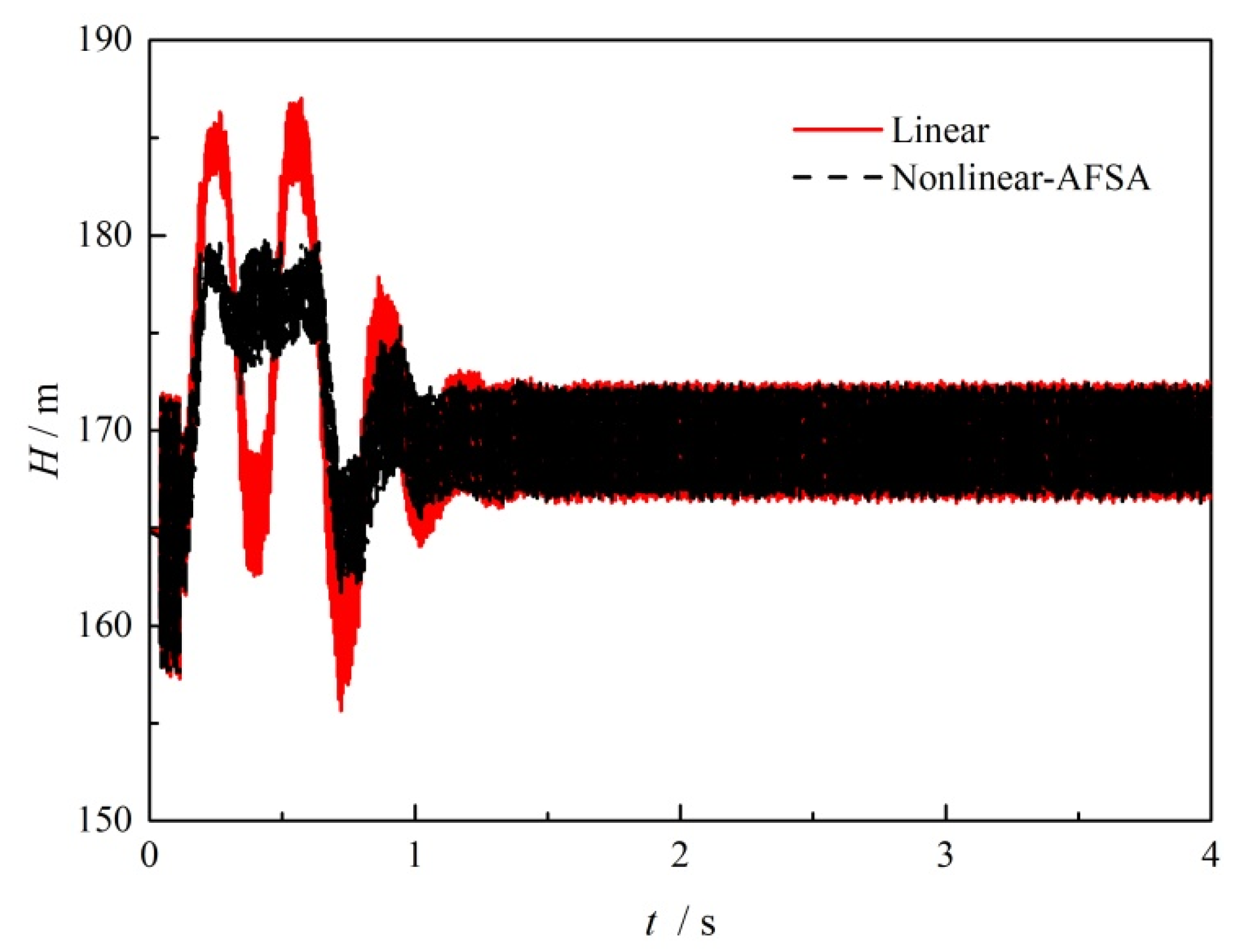
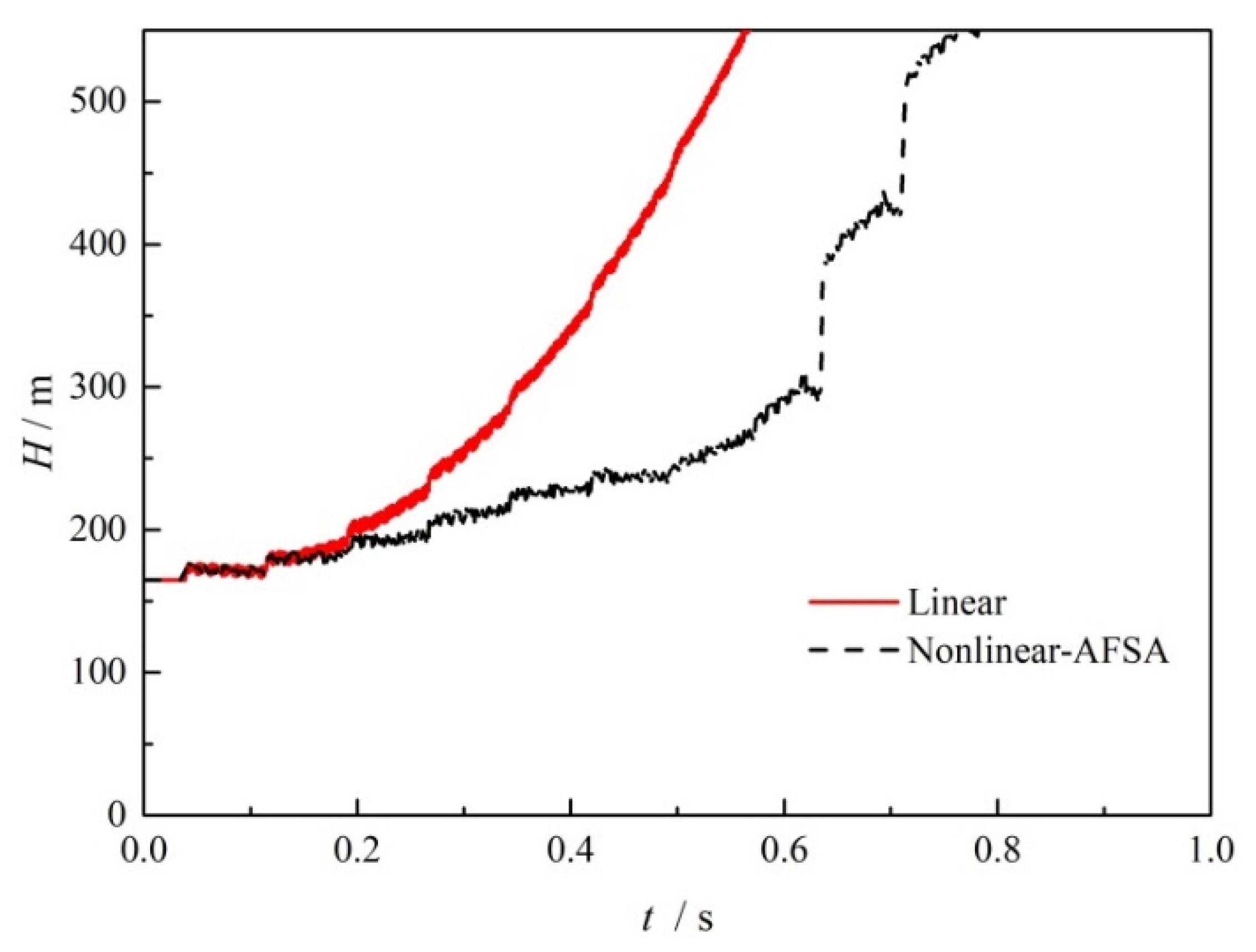
The transient wave surge can be reduced through nonlinear valve closure without adding additional damping devices. For transient flow with and without a centrifugal pump running, surge reduction of 9.3% and 11.4% could be obtained in the most severe valve closure case. Even with increasing pressure with positive displacement pump operation, the surge damping method was able to achieve a 34% time margin for reaching the head limit and a maximum reduction in the surge amplitude of 75.2%.

(2)

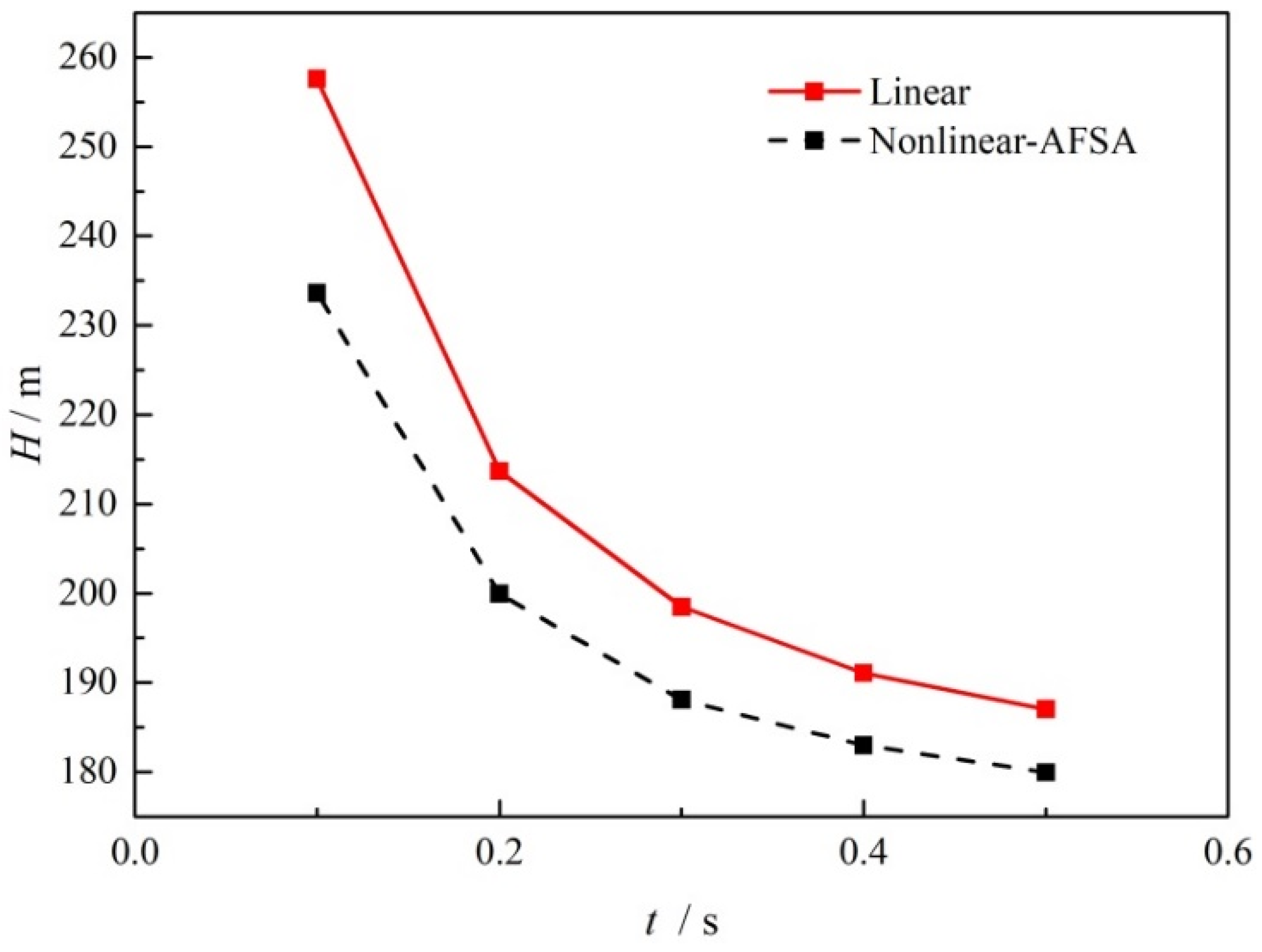
With increasing valve closing time, the surge amplitude caused by valve closure decreases for the transient flow with and without the centrifugal pump running, and the rate of surge amplitude decrease also decreases. For positive displacement pumps, the surge amplitude increases with increasing valve closing time, but at a significantly slower rate of increase with the optimized nonlinear valve closure.

(3)

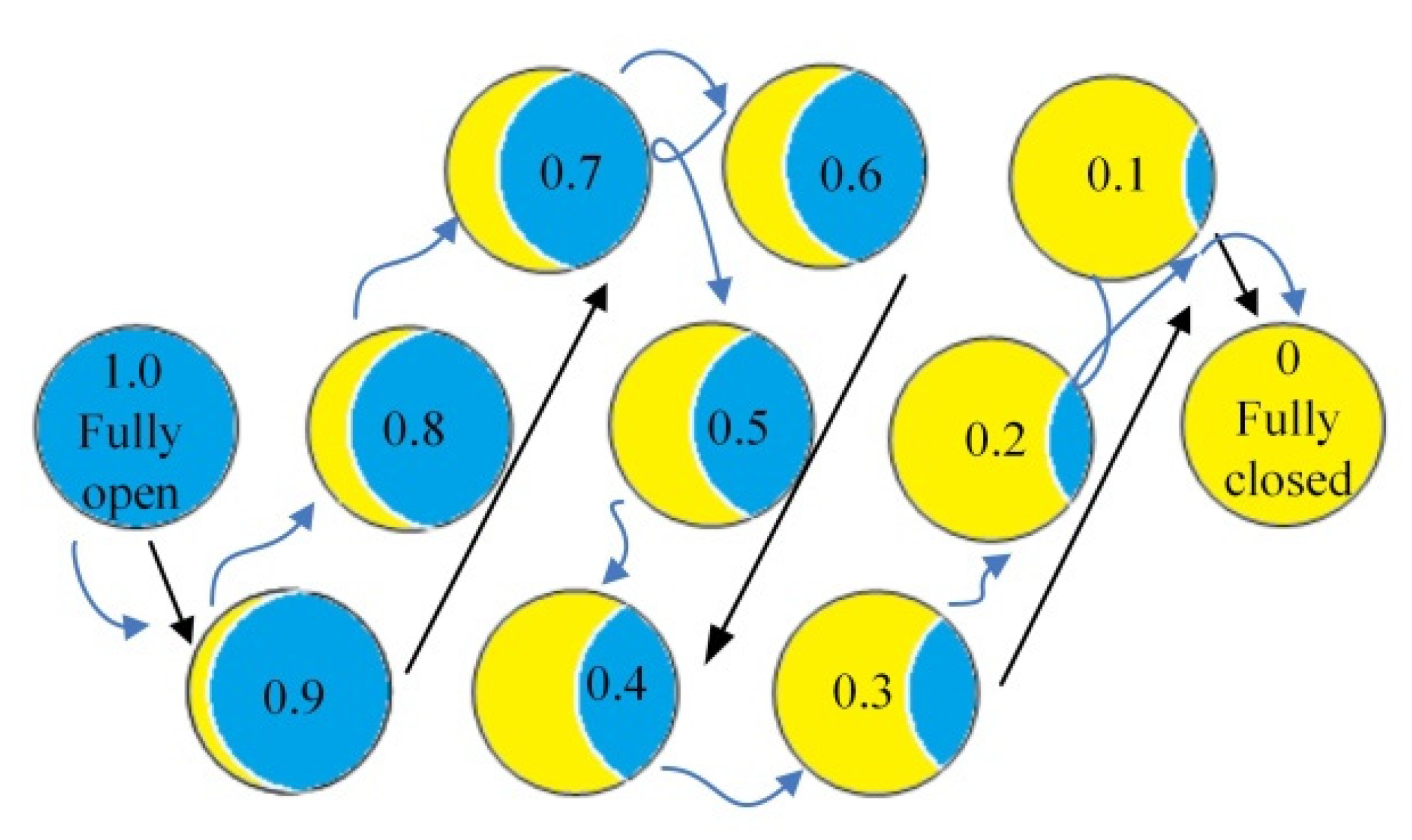
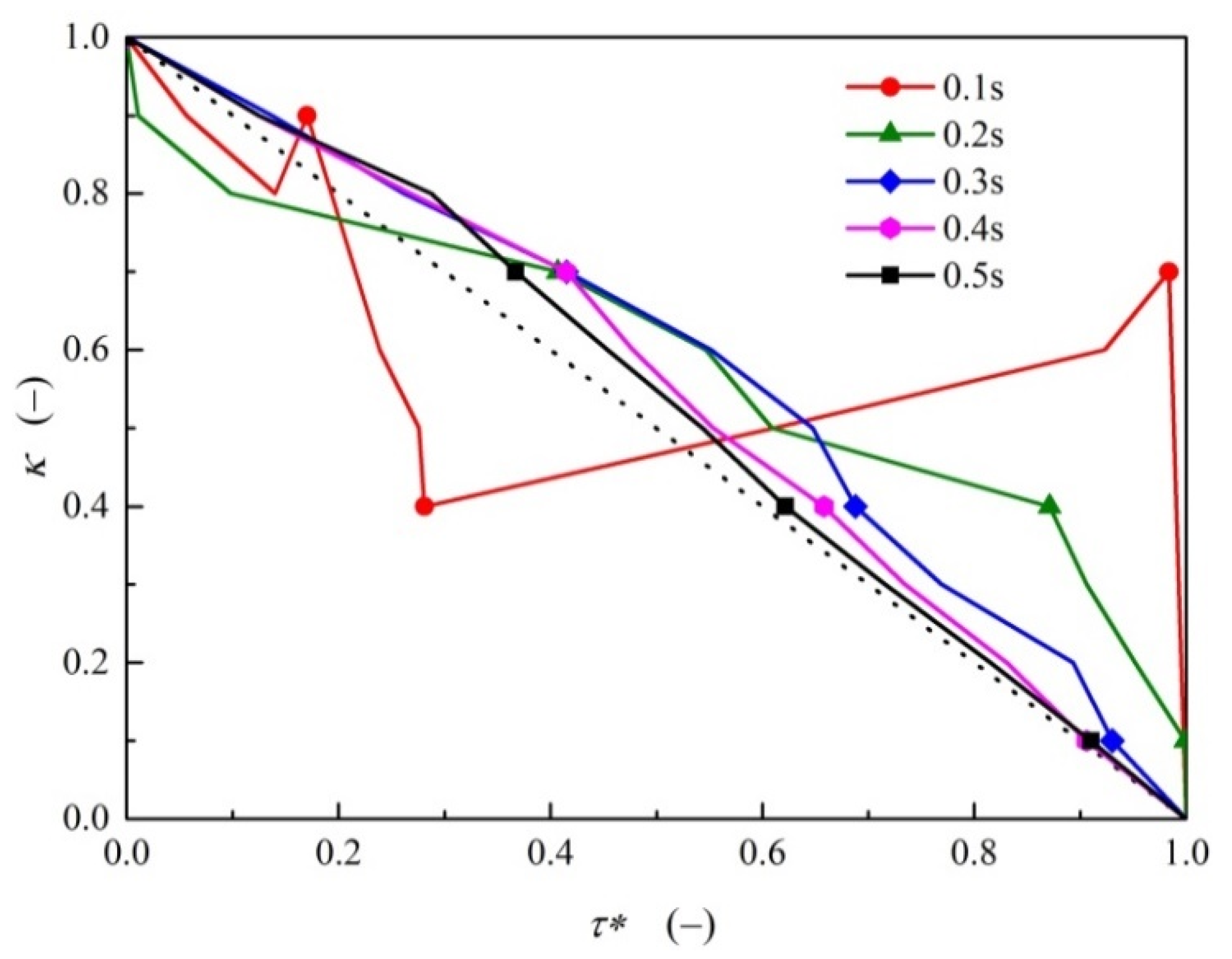
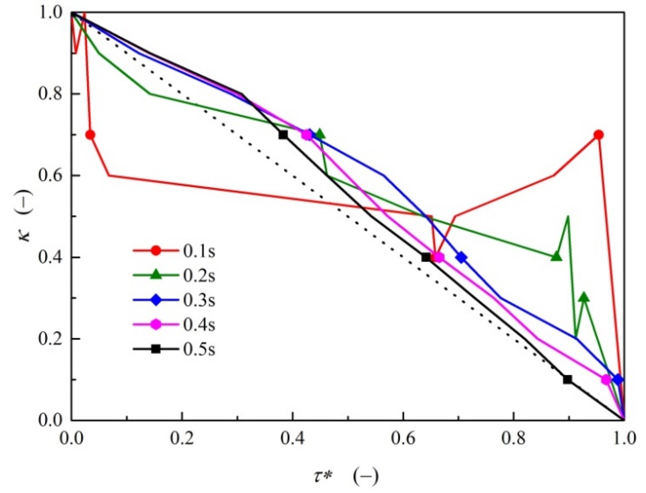
For rapid valve closure in 0.1 s, the optimized nonlinear closing motion performs a similar “И” shape. For other valve closure cases in the present study, the optimized valve opening curves show a relatively smooth variation during the initial stage before decreasing rapidly to full closure during valve operation.

(4)

The valve closure process can be abstracted into a traveling salesman problem, and further optimization using an artificial fish swarm algorithm was demonstrated to be beneficial for wave damping. The strategy proposed in the present study could help for either guiding real-time valve control or serve as a design reference for novel valve structures for the purpose of surge protection.

References

1. Mandhare, N.A.; Karunamurthy, K.; Ismail, S. Compendious Review on “Internal Flow Physics and Minimization of Flow Instabilities Through Design Modifications in a Centrifugal Pump”. ASME J. Press. Vessel. Technol. 2019, 141, 051601. [Google Scholar] [CrossRef]
2. Tanaka, T.; Tsukamoto, H. Transient behavior of a cavitating centrifugal pump at rapid change in operating conditions—Part 1: Transient phenomena at opening/closure of discharge valve. ASME J. Fluids Eng. 1999, 121, 841–849. [Google Scholar] [CrossRef]
3. Duan, H.F.; Lee, P.J.; Che, T.C.; Ghidaoui, M.S.; Karney, B.W.; Kolyshkin, A.A. The influence of non-uniform blockages on transient wave behavior and blockage detection in pressurized water pipelines. J. Hydro-Environ. Res. 2017, 17, 1–7. [Google Scholar] [CrossRef]
4. Duan, H.F.; Ghidaoui, M.S.; Lee, P.J.; Tung, Y.K. Relevance of unsteady friction to pipe size and length in pipe fluid transients. J. Hydraul. Eng. 2012, 138, 154–166. [Google Scholar] [CrossRef]
5. Ghidaoui, M.; Mansour, S.; Zhao, M. Applicability of quasi steady axisymmetric turbulence models in water hammer. J. Hydraul. Eng. 2002, 128, 917–924. [Google Scholar] [CrossRef]
6. Zielke, W. Frequency-dependent friction in transient pipe flow. J. Basic Eng. 1968, 90, 109–115. [Google Scholar] [CrossRef]
7. Urbanowicz, K. Fast and accurate modelling of frictional transient pipe flow. Z. Angew. Math. Mech. 2018, 5, 802–823. [Google Scholar]
8. Trikha, A.K. An efficient method for simulating frequency dependent friction in transient liquid flow. J. Fluids Eng. 1975, 97, 97–105. [Google Scholar] [CrossRef]
9. Vardy, A.E.; Brown, J.M.B. Transient turbulent friction in fully rough pipe flows. J. Sound Vib. 2004, 270, 233–257. [Google Scholar] [CrossRef]
10. Zarzycki, Z.; Kudzma, S. Simulation of transient flows in a hydraulic system with a long liquid line. J. Theor. App. Mech. 2007, 45, 853–871. [Google Scholar]
11. Vitkovsky, J.P.; Stephens, M.; Bergant, A.; Simpson, A.R.; Lambert, M.F. Numerical error in weighting function-based unsteady friction models for pipe transients. J. Hydraul. Eng. 2006, 132, 709–721. [Google Scholar] [CrossRef] [Green Version]
12. Brunone, B.; Golia, U.M.; Greco, M. Effects of two dimensionality on pipe transients modeling. J. Hydraul. Eng. 1995, 121, 906–912. [Google Scholar] [CrossRef]
13. Pezzinga, G. Evaluation of Unsteady Flow Resistances by Quasi-2D or 1D Models. J. Hydraul. Eng. 2000, 126, 778–785. [Google Scholar] [CrossRef]
14. Ramos, H.; Covas, D.; Borga, A.; Loureiro, D. Surge damping analysis in pipe systems: Modelling and experiments. J. Hydraul. Res. 2004, 42, 413–425. [Google Scholar] [CrossRef]
15. Duan, H.F.; Meniconi, S.; Lee, P.J.; Brunone, B.; Ghidaoui, M.S. Local and integral energy-based evaluation for the unsteady friction relevance in transient pipe flows. J. Hydraul. Eng. 2017, 143, 04017015. [Google Scholar] [CrossRef] [Green Version]
16. Nault, J.D.; Karney, B.W. Comprehensive adaptive modelling of 1-D unsteady pipe network hydraulics. J. Hydraul. Res. 2021, 59, 263–279. [Google Scholar] [CrossRef]
17. Cao, Z.; Wang, Z.; Deng, J.; Guo, X.; Lu, L. Unsteady friction model modified with compression–expansion effects in transient pipe flow. AQUA—Water Infrastruct. Ecosyst. Soc. 2022, 71, 330–344. [Google Scholar] [CrossRef]
18. Wu, D.; Yang, S.; Wu, P.; Wang, L. MOC-CFD coupled approach for the analysis of the fluid dynamic interaction between water hammer and pump. J. Hydraul. Eng. 2015, 141, 06015003. [Google Scholar] [CrossRef]
19. He, L.; Wen, K.; Gong, J.; Wu, C. A multi-model ensemble digital twin solution for real-time unsteady flow state estimation of a pumping station. ISA Trans. 2021. online ahead of print. [Google Scholar] [CrossRef]
20. Vítkovský, J.P.; Bergant, A.; Simpson, A.R.; Lambert, M.F. Systematic evaluation of one-dimensional unsteady friction models in simple pipelines. J. Hydraul. Eng. 2006, 132, 696–708. [Google Scholar] [CrossRef] [Green Version]
21. Bettaieb, N.; Taieb, E.H. Assessment of failure modes caused by water hammer and investigation of convenient control measures. J. Pipeline Syst. Eng. Pract. 2020, 11, 04020006. [Google Scholar] [CrossRef]
22. Garg, R.K.; Kumar, A.; Abbas, A. Analysis of wave damping in pipeline having different pipe materials configuration under water hammer conditions. Res. Sq. 2021, 1–30. [Google Scholar] [CrossRef]
23. Urbanowicz, K.; Stosiak, M.; Towarnicki, K.; Bergant, A. Theoretical and experimental investigations of transient flow in oil-hydraulic small-diameter pipe system. Eng. Fail. Anal. 2021, 128, 105607. [Google Scholar]
24. Wan, W.; Huang, W. Investigation on complete characteristics and hydraulic transient of centrifugal pump. J. Mech. Sci. Technol 2011, 25, 2583–2590. [Google Scholar] [CrossRef]
25. Wang, X.; Zhang, J.; Chen, S.; Shi, L.; Zhao, W.; Wang, S. Valve closure based on pump runaway characteristics in long distance pressurized systems. AQUA—Water Infrastruct. Ecosyst. Soc. 2021, 70, 493–506. [Google Scholar] [CrossRef]
26. Tian, W.; Su, G.H.; Wang, G.; Qiu, S.; Xiao, Z. Numerical simulation and optimization on valve-induced water hammer characteristics for parallel pump feedwater system. Ann. Nucl. Energy 2008, 35, 2280–2287. [Google Scholar] [CrossRef]
27. Triki, A.; Essaidi, B. Investigation of Pump Failure-Induced Waterhammer Waves: A Case Study. J. Press. Vessel Technol. 2022, 144, 061403. [Google Scholar] [CrossRef]
28. Sattar, A.M.A.; Soliman, M.; El-Ansary, A. Preliminary sizing of surge vessels on pumping mains. Urban. Water J. 2019, 16, 738–748. [Google Scholar] [CrossRef]
29. Kubrak, M.; Malesińska, A.; Kodura, A.; Urbanowicz, K.; Bury, P.; Stosiak, M. Water Hammer Control Using Additional Branched HDPE Pipe. Energies 2021, 14, 8008. [Google Scholar] [CrossRef]
30. Bostan, M.; Akhtari, A.A.; Bonakdari, H.; Gharabaghi, B.; Noori, O. Investigation of a new shock damper system efficiency in reducing water hammer excess pressure due to the sudden closure of a control valve. ISH J. Hydraul. Eng. 2020, 26, 258–266. [Google Scholar]
31. Triki, A.; Trabelsi, M. On the in-series and branching dual-technique-based water-hammer control strategy. Urban. Water J. 2021, 18, 631–639. [Google Scholar] [CrossRef]
32. Triki, A. Comparative assessment of the inline and branching design strategies based on the compound-technique. AQUA-Water Infrastruct. Ecosyst. Soc. 2021, 70, 155–170. [Google Scholar] [CrossRef]
33. Reddy, H.P.; Araya, W.F.; Chaudhry, M.H. Estimation of decay coefficients for unsteady friction for instantaneous, acceleration-based models. J. Hydraul. Eng. 2012, 138, 260–271. [Google Scholar] [CrossRef]
34. Guo, X.; Zhu, Z.; Shi, G.; Huang, Y. Effects of rotational speeds on the performance of a centrifugal pump with a variable-pitch inducer. J. Hydrodynam. 2017, 29, 854–862. [Google Scholar] [CrossRef]
35. Chaudhry, M.H. Applied Hydraulic Transients; Springer: New York, NY, USA, 2014. [Google Scholar]
36. Barrio, R.; Blanco, E.; Keller, J.; Parrondo, J.; Ferna’ndez, J. Numerical determination of the acoustic impedance of a centrifugal pump. In Proceedings of the Fluids Engineering Division Summer Meeting, Hamamatsu, Japan, 24–29 July 2011; pp. 405–412. [Google Scholar]
37. Hu, J.; Yang, J.; Zeng, W.; Yang, J. Transient pressure analysis of a prototype pump turbine: Field tests and simulation. J. Fluids Eng. 2018, 140, 071102. [Google Scholar]
38. Zhang, J.; Yang, H.; Liu, H.; Xu, L.; Lv, Y. Pressure Fluctuation Characteristics of High-Speed Centrifugal Pump with Enlarged Flow Design. Processes 2021, 9, 2261. [Google Scholar] [CrossRef]
39. Li, X. A new Intelligent Optimization Method-Artificial Fish School Algorithm. Ph.D. Thesis, Zhejiang University, Hangzhou, China, 2003. (In Chinese). [Google Scholar]
40. Adamkowski, A.; Lewandowski, M. Experimental examination of unsteady friction models for transient pipe flow Simulation. J. Fluids Eng. 2006, 128, 1351. [Google Scholar] [CrossRef]
41. Azizi, R. Empirical study of artificial fish swarm algorithm. Int. J. Comput. Netw. Commun. 2014, 3, 1–7. [Google Scholar]
42. Martin, C.S. Representation of Pump Characteristics for Transient Analysis. In Proceedings of the ASME, Symposium on Performance Characteristics of Hydraulic Turbines and Pumps, Winter Annual Meeting, Boston, MA, USA, 13–18 November 1983; pp. 1–13. [Google Scholar]
43. Donsky, B. Complete pump characteristics and the effects of specific speeds on hydraulic transients. J. Basic Eng. 1961, 83, 685–696. [Google Scholar]
Figure 1. Discrete grids of the pipeline system.
Water 14 01576 g001
Figure 2. Valve shut-off procedures with optimized fish results.
Water 14 01576 g002
Figure 3. Conceptual optimization process of the designed artificial fish.
Water 14 01576 g003
Figure 4. The calculation flow chart for the surge damping optimization. (a) Optimization procedures using ASFA; (b) Hydraulic transient calculation procedures.
Water 14 01576 g004
Figure 5. Head comparison with experimental data at the pipe’s midpoint.
Water 14 01576 g005
Figure 6. Validation results using different test functions. (a) optimization for sphere function; (b) optimization for Rosenbrock function; (c) optimization for Schwefel function.
Water 14 01576 g006
Figure 7. Observation of the distribution of artificial fish in the optimization process.
Water 14 01576 g007
Figure 8. The fitness function and convergence curve of the optimization process.
Water 14 01576 g008
Figure 9. Comparison of the pressure fluctuation with a valve closing time of 0.1 s with no pump operation.
Water 14 01576 g009
Figure 10. Comparison of the pressure fluctuation with a valve closing time of 0.5 s with no pump operation.
Water 14 01576 g010
Figure 11. Pressure surge amplitude for different valve closing times with no pump operation.
Water 14 01576 g011
Figure 12. Optimized valve operation characteristics with no pump operation.
Water 14 01576 g012
Figure 13. Comparison of the pressure fluctuation with a valve closing time of 0.1 s with centrifugal pump operation.
Water 14 01576 g013
Figure 14. Comparison of the pressure fluctuation with a valve closing time of 0.5 s with centrifugal pump operation.
Water 14 01576 g014
Figure 15. Pressure surge amplitude at different valve closing times with centrifugal pump operation.
Water 14 01576 g015
Figure 16. Optimized valve operation characteristics with centrifugal pump operation.
Water 14 01576 g016
Figure 17. Comparison of the pressure rise in 0.1 s valve closing time with positive displacement pump operation.
Water 14 01576 g017
Figure 18. Comparison of the pressure increase with a 0.5 s valve closing time with positive displacement pump operation.
Water 14 01576 g018
Figure 19. Pressure surge amplitude at different valve closing times with positive displacement pump operation.
Water 14 01576 g019
Figure 20. Optimized valve operation characteristics with positive displacement pump operation.
Water 14 01576 g020