Article

Key Factors for the Findability of Fish Passes in Large Epipotamal Rivers: The Case of the River Drava

1
Institute of Hydraulic Engineering and River Research (IWA), Department of Water, Atmosphere and Environment (WAU), University of Natural Resources and Life Sciences (BOKU) Vienna, 1180 Vienna, Austria
2
Institute of Statistics (STAT), Department of Landscape, Spatial and Infrastructure Sciences, University of Natural Resources and Life Sciences (BOKU) Vienna, 1180 Vienna, Austria
3
VERBUND Hydro Power GmbH, 1011 Vienna, Austria
*
Author to whom correspondence should be addressed.
Water 2022, 14(10), 1530; https://doi.org/10.3390/w14101530
Submission received: 1 April 2022 / Revised: 6 May 2022 / Accepted: 7 May 2022 / Published: 10 May 2022
(This article belongs to the Special Issue Large Rivers in a Changing Environment)

Abstract

:
Restoring the longitudinal connectivity of rivers through fish passes is of great importance for achieving good ecological status of surface waters. However, the key stimuli determining the findability of the entrance of these structures is still subject to debate. In this article, the influence of water temperature, light and acoustic stimuli in addition to flow parameters on fish movement is assessed. Analyses are based on a comprehensive dataset of 40,000 fish migrations covering time accurate recording of ascending individuals during the observation periods from 2015 to 2020 in various fish passes on the river Drava in Carinthia, Austria. The data are assessed by technical, fish ecological and statistical methods. Results indicate that the effect of the water temperature gradient between the fish pass and the main river has most impact on the ascent rates, whereas the two factors of light and acoustic, as well as most of the flow parameters, have no or negligible effect on the findability. A favourable thermal environment can be important to ensure efficient upstream migration and thus facilitate the findability of fish passes.

1. Introduction

“There doesn’t exist any completely untouched river in the Alpine arc, even larger near-natural sections are rare today” [1]. This statement from 1992 is applicable to almost the whole of Europe and the USA. The pervasive alteration of riverine ecosystems worldwide, due to their development for human needs, represents one of the greatest and priority challenges for the preservation and restoration of the fish fauna [2,3,4,5,6]. Obstacles that prevent or restrict the migration of fish, such as dams and weirs, isolate and alter previously connected fish communities, leading to drastic changes in the structure of the faunal communities of freshwater ecosystems and loss of biodiversity [7,8,9]. The European Water Framework Directive demands the maintenance or establishment of “good ecological status” for water bodies, defined by biological, hydromorphological, chemical and physical-chemical elements [10]. The main issue we have to deal with in Europe regarding the “good ecological status” is, without a doubt, the hydromorphological element, and here in particular, in a very high percentage, is the longitudinal connectivity. For decades, fish passes have been the most important means to re-establish the river continuum at the barriers; it is, therefore, not surprising that many publications, consisting of handbooks, guidelines and technical papers, have been published on the operation and design of fish passes [11,12,13,14,15]. There is a vast number of thresholds, reference or guiding values in those guidelines. However, most of them have never been evaluated regarding their ecological relevance [16].
One essential point in the design of fish passes concerns the findability of the entrance. The two major factors influencing findability are the position of the entrance in relation to the obstacle, and the presence of conditions that attract fish, respectively, and “guide” them towards the fish pass. The importance of the correct position of the entrance was first mentioned in 1912 [17]. It has since been discussed and further specified in numerous publications and is essentially undisputed. Attraction factors, on the other hand, target fish behaviour, e.g., rheotaxis, phonotaxis, phototaxis, chemotaxis and thermotaxis, to mention a few [18,19,20,21]. Despite the wide range of possible influencing factors, there is a lack of large-scale field studies that relate these factors to the findability of the fish migrating facilities.
The physical factor most frequently mentioned in the literature is the flow situation in the entry area, which is mainly determined by flow velocity, turbulence and flow impulse. The flow velocity is bounded upwards by the swimming performance of the weakest individuals, and downwards by the minimum velocity perceptible to fish. For the lower bound, values from the literature range from about 0.15 m/s for juvenile fish and 1.25 m/s for adult salmonids [22,23]. The flow impulse can only be controlled by the amount of water exiting the fish pass. Nevertheless, the magnitude of this impulse and thus of the attraction flow cannot be considered independently, as it is perceived to act relative to the competing flow over the weir or the turbines. Hence, Austrian and European Guidelines request an attraction flow at fish pass entrances at approximately 1–5% of the competing flow of the river, based on Larinier et al. [24].
Another major factor attracting fish and affecting its behaviour is the water temperature. It is well known that water temperature is one of the main triggers for fish migration. It influences the oxygen level of the water body, the trophic status and thus also nutrient availability for water organisms, and has therefore major influence on the energy balance and migration behaviour of fish [25].
In this work, we analyse the data of three function monitoring projects that took place over a timespan of five years at different fish passes in the epipotamal of the Drava River in Carinthia/Austria. Temperature, natural light conditions and flow data were recorded at each of the fish passes; furthermore, two additional artificial stimuli, addressing the phonotaxis and the phototaxis, were set at one single site. The following research questions will be addressed: (1) do the variables under investigation have a significant effect on the ascent rates; (2) can this influence be quantified in terms of effect size or incident rate ratios; and (3) does the influence vary between families, guilds and species, in terms of significance and/or effect size.
The collected data were sufficient to affirm our three principal hypotheses: (1) that the findability of the entrance is not or just weakly correlated to the flow parameters in the fish pass; (2) that the effect size of temperature parameters far outweighs that of the flow parameters of the main river; and (3) that there is a difference in response to the key factors between different families, flow preference guilds and species.
We use and compare the standard frequentist with the Bayesian statistical approaches to test the plausibility of the results of the regression analyses.

2. Materials and Methods

2.1. Study Site

The monitoring projects were carried out at fish passes at the Hydro Power Plants (HPP) Lavamünd, Schwabeck and Edling, situated at river Drava in Carinthia/Austria (Figure 1). The Drava, with a catchment area of about 12,000 square kilometres, drains the whole of Carinthia and East Tyrol and is thus an essential part of the Danube catchment area south of the main Alpine ridge. It is one of the most exploited rivers in the world in terms of hydropower, with 11 hydro power stations on the length of 270 km on its way through Austria (Figure 2). The HPP chain shows overlapping reservoirs. Therefore, the influence of the flow regulation and energy generation just show insignificant alterations in water level at the entrance of the fish passes. The tailwater of the single HPPs is mainly affected by the headwater of the downstream HPP.
Currently, the entire chain of power plants is being equipped with fish passes to restore the river continuum and thus fish passability. The optimal position of the entrance to each fish pass was determined using 2D hydraulic simulations. The entrances are located where a directed flow without rotating swivels downstream the turbines meets the riverbank, and are in all three cases situated at the end of the construction bay of the HPP. During the construction of these fish passes, the current research project, supported by VERBUND Hydro Power GmbH, was initiated, in which different key stimuli for finding the entrances of fish passes are investigated.
The three fish passes considered are vertical slot passes of the type enature® and are located in the epipotamal fish region with the lead species Squalius cephalus, Barbus barbus, Chondrostoma nasus and Hucho hucho [27].
The total lengths of the fish passes vary between 300 m and 650 m, with the fish pass at HPP Edling being the longest. The distance of the entrance varies between 110 m to 150 m to the obstacle, with an angle of about 35° between the flow direction of the watercourse and the outflow direction of the fishway. Table 1 provides an overview of the characteristics of the individual study sites.

2.2. Data Acquisition

Data were collected over various time periods across the three sites (Table 2), from 2015 to 2017 and from 2019 to 2020, with a total of 776 days of monitoring. Subsequently, the data acquisition will be split up into two parts, which will be mentioned separately:
  • The measured and derived predictor variables.
  • The fish ecological monitoring.

2.2.1. Predictor Variables

The discharge data of the main channel of the Drava (Qd) were provided by VERBUND Hydro Power GmbH with a temporal resolution of 15 min. The discharge in the fish passes (Qf) varied depending on the headwater level of the Drava and was thus almost independent of the runoff in the main channel. It was calculated in 15 min time intervals, using a rating curve and the data of the headwater level of the river Drava. The combination of the varying discharge in the river Drava caused by hydro peaking at the three HPPs and the change in discharge in the fish pass led to a guiding flow (Qa) in the range of 0.03 to >400% of the competing flow throughout the period of this study. Qa was calculated according to (1):
Qa = Qf × 100/Qd
Extreme values of the guiding flow (of more than 10% of Qd) occurred during the periods when the turbines of the HPPs were not in operation and the natural discharge of the Drava was intermitted and stored in the reservoirs for later energy production. About 750 hourly data sets scattered over the entire study period were affected. As there was just a minor influence on the water level at the entrance, because the water surface elevation (WSEL) is mainly dependent from the storage level of the downstream HPP in the chain with overlapping reservoirs, the WSEL at the entrance was not considered as a relevant and independent predictor variable. The discharge of the river Drava and one of the fish passes are at considerable different orders of magnitude, which hampers the comparability of results. Qd and Qf were therefore scaled so that a change of one unit corresponds to a change of 10% of the mean discharge in each case, which is 275 m3/s for the river Drava and 0.038 m3/s for the fish passes.
Water temperature was recorded by temperature sensors in time intervals of 1 h. The sensors with data logger of type “onset® HOBO® U22 Pro v2” were positioned in the most downstream pool of the fish pass, as well as in the main channel of the river Drava (Table 3).
Since the temperature shows a distinctly sinusoidal characteristic over the course of the year, and fish migration starts in spring when the water temperature rises and ends again towards winter when water temperature drops and fish move to their winter habitats, it seemed reasonable to consider a seasonal trend when analysing the effect of water temperature on ascent rates. For this purpose, a seasonal trend adjustment was carried out by fitting a sine curve to the annual cycle of the mean daily water temperature of the river Drava from 2017–2019. The temperature data used in the analysis stem from a gauge situated only 300 m downstream the HPP Lavamünd and can therefore be considered representative for the study area. The residuals of this adjustment process were used as the predictor variable “water temperature residuals” (tres) in the further analyses. The variable “water temperature difference” (tdiff), on the contrary, denotes the difference between the water temperature in the direct entry area of the fish pass and the water temperature of the river Drava without sinusoidal adjustment. The idea behind this is that the physical properties of water, such as density and especially kinematic viscosity, change with temperature. The mixing processes between two water bodies are thus influenced by the temperature gradient, resulting in a thermal front from the fish pass into the river, which can be perceived by the fish in their migrating corridor.
The “season” (seas) as a categorical predictor variable was considered, as there are differences in spawning- and thus migration times between the 34 observed species, some of which were subsequently analysed separately.
Since the study spanned 5 years of observations, the variable “year” addresses the fact that the number of migrating fish varies from year to year. This variation is based on influences not considered here, such as extreme floods and turbidity, among others, that have a strong impact on migration and are capable of destroying downstream habitats, as well as entire populations of juvenile fish and larvae [28,29]. The unobserved differences between the three locations of the fish passes were represented in the statistical models by the categorial variable “site”.
At one site, at the HPP Edling, light and acoustic were set manually as key stimuli during the spring and autumn monitoring in 2019 from 19 April 2019 to 18 June 2019 and from 17 September 2019 to 4 November 2019. This was to investigate the phototactic and phonotactic behaviour of the fish to determine whether these manually placed stimuli have an influence on the ascent rates and the findability of the fish pass entrance. The light stimulus was set by three LED strips with 630 lm/m and a total length of 15 m, which were positioned downstream from the first pool of the fish pass on both sides of the bank (Figure 3). The LED strips with a beam angle of about 110° were fixed about one meter above the ground. The resulting illuminance was about 50–100 lux, depending on the turbidity in the Drava. The acoustic stimulus was set by two under water speakers, which were positioned in the entrance area of the fish pass. The signal, played through an amplifier in a loop, was recorded in the preliminary study at a spawning location, known to be passed by many fish. The recording was made, using a calibrated measurement chain consisting of a Teledyne Reson TC4034 hydrophone, the corresponding Teledyne Reson EC6067 preamplifier and a Norsonic NOR140 Class I sound level meter. The volume of the signal was chosen to correspond to the sound pressure level at the recording location [30].
The artificial key stimuli acoustics and light were each constant for 24 h and changed in a pre-programmed weekly pattern from Monday to Sunday, according to Table 4.

2.2.2. Fish Ecological Monitoring

To evaluate the migration potential, the fish population downstream one of the weirs was recorded once during the monitoring period by electrofishing from the boat and by wading with a backpack DC power unit. In total, an area of 6.3 ha subdivided in 60-day and 21-night stripes in the river Drava and within the fish pass in 51 pools and 6 resting areas with a total area of 400 m2 have been targeted [16,31]. Out of the relation between the body lengths of different species to their spawning ripeness [27], a selection of the targeted fish into two groups, either if they are or are not ready to migrate and spawn, was conducted. Based on this, the theoretical migration potential was calculated. The species observed during this evaluation are shown in Table 5.
For the monitoring itself, the FishCam-System [32], consisting of a camera unit and a detection tunnel with a back wall, and a structured bottom and a mirror cover to determine the length of the passing fish, was applied. With two of these monitoring systems per site, the ascending individuals were recorded once near the entrances of the fish passes and once near the exits. The data under consideration relate to the cameras at the entrances. The migrating fish did thereby not experience any stress during the recording, as they were neither touched nor haltered. The time of migration of the fish was recorded by a time stamp in the video signature. The time stamp is a requirement to ensure that the time of fish entry into the fish pass can be accurately associated with all the independent variables. The recorded videos were stored and post- processed with FishNet, a software, that filters videos with fish from that with any other moving objects [33]. Finally, the determination of fish species is carried out by fish biologists. To avoid the occurrence of multiple records in the data, records with similar timestamps and migrations in different directions were looked at more closely and filtered in the case of duplications. Comparing the sum of fish entering the fish pass with the one leaving it at the exits, gave us a good overview over the number of ascending fish, although there were minor differences in the totals.

2.3. Data Processing

All data constitute time series, with gaps at the times when no monitoring took place. The data were aggregated to one-hour time intervals, to reduce the amount of data to a meaningful level without influencing the characteristics of the predictor variables too much. The fish data were cumulated in their entirety on the one hand and subdivided into individual subgroups on the other. We have chosen to distinguish the sub-groups both by family and by membership of one of the flow preference guilds according to Schiemer et al. [34]. Four selected species with high abundance were evaluated separately, including the two lead species, Chub (Squalius cephalus) and Nase (Chondrostoma nasus), Bleak (Alburnus alburnus) as the species with the highest abundance, and Roach (Rutilus rutilus). Alburnus alburnus were not included in the sub-groups of families and flow preference guilds, as their high abundance of over 55% would have severely biased the results of these sub-groups. The analyses for all the sub-groups were conducted at a one-hour time interval, as well as on a three-hour, six-hour and daily time interval, to examine the influence of the diurnal variation of some predictor variables on the model results.

2.4. Statistical Methods

Statistical analysis was conducted using two fundamentally different statistical methods for the regression analyses. The starting point was the standard frequentist approach to regression modelling, followed by Bayesian models for plausibility verification. Mixed-models were used in both approaches to determine the relationship between ascent rates and the independent variables. The models include the variable “year” as a random effect, whereas all other variables were defined as fixed effects. The reason for that was that we have only measured sub-sets of possible years at each site, and treating the year as a random effect allowed accounting for between-year variation. The boxplot in Figure 4 shows the variation of the daily ascent rates across the years. Complete pooling (ignoring year as variable) would ignore variation between the years, whereas the no-pooling analysis (setting year as fixed effect) would overstate it and tends to overfit the data within each year [35]. The partial-pooling model (mixed effects model), in contrast, captures the expected similarities that ascent rates share between years and adjusts the model to an annual magnitude of the predictors. To avoid overparameterization, which can lead either to uninterpretable models, or to convergence issues [36,37], which also occurred during test model setups, we restricted the effect of the random variable to the intercept only and did not model the random slope.
Since the response variable is count data (number of ascending individuals per time unit), generalized linear mixed model framework needs to be adapted [38]. In a preliminary assessment, we tested the suitability of three different distributions: the Poisson, the negative-binomial [39] and the zero-inflated-negative-binomial distribution. The Poisson distribution showed severe overdispersion and was therefore rejected, whereas negative-binomial and zero-inflated-negative-binomial distributions showed equally good results in predicting the observed values. For reasons of model simplicity and interpretability, we opted for the negative-binomial distribution for further statistical analyses.
The null-hypotheses are that the predictor variables have no significant influence on the ascent rates.
The estimates of the frequentist mixed-models were tested with a likelihood ratio test on a significance level of α = 0.05. We assessed the collinearity of independent variables using the variance inflation factor (VIF) and checked model assumptions using scaled residual plots [40].
The same set of fixed- and random-effect variables was applied to the Bayesian model approach. The multilevel models were fitted using the brms package [41] in R, which performs a Markov Chain Monte Carlo approximation with the No U-Turn Sampler to approximate the posterior distributions of the model parameters. For each model, we used 4 chains, each with 5000 iterations with the warmup phase including 1000 iterations; the maximum treedepth was set to 20, as in the first simulations, and there were a number of transitions that exceeded the default maximum number, which can bias the posterior draws. The family was set to negative-binomial, and the default priors were used for the standard deviation of the random effects. On the fixed-effect categorial variables, we set weakly informative priors, and on the variables of the flow and temperature parameters, we set informative priors. Stationarity of the posterior distribution was reached when the potential scale reduction factor (Rhat) was smaller than 1.01, which indicated convergence of the chains [42]. The posterior distributions of the model parameters are summarized using the posterior means and the 95% equal-tailed credible intervals. The fitted models were checked in terms of convergence, autocorrelation, and the quality of the posterior predictive distribution. The full models are presented with confidence intervals of the estimates and p-values for the frequentist models.
The statistical analyses for both approaches were carried out for various groups of different sizes: all individuals (nall), the flow preference guilds of the rheophilic (nrheo) and the eurytopic without the Bleak (neury), the families of the Salmonidae (nsal), the Percidae (nper) and the Cyprinidae (ncyp) without the Bleak, as well as the species Bleak (Alburnus alburnus—nlau), Nase (Chondrostoma nasus—nnas), Bream (Abramis brama—nbra) and Chub (Squalius—nait).
In a more detailed assessment, focusing on acoustics and light, these two parameters were investigated at the fish pass at the HPP Edling during the spring and autumn monitoring in 2019. For this purpose, the 24-h data for each of the two variables were divided into two groups. “Stimulus” referred to those where light or acoustics was set, and “without stimulus” referred to the rest. The difference between the two groups with respect to ascent rates of “all individuals” (nall), flow preference guilds (nrheo, neury) and families (ncyp, nsal, nper) were assessed using the Mann–Whitney U-tests. The dataset for this assessment was first categorised by the variable “daylight”, which was derived from the timestamp. For the subsequent evaluation, only the data without daylight were used, as the artificial light source is very unlikely to have any influence during daytime.
Table 6 provides an overview over the predictor variables for the statistical analyses.

3. Results

3.1. FishCam Monitoring

Across the entire study, a total of 18,456 one-hour observations were recorded on 776 days at the three sites. In this time, 40,194 fish migrated through the fish passes under various environmental conditions. We could observe 39 different species. Of the four lead species stated in the guideline, Chub (Squalius cephalus), Barbel (Barbus barbus) and Nase (Chondrostoma nasus) passed through the fish passes. Only the Danube Salmon (Hucho hucho) was not detected. Of the typical species, only Western vairone (Telestes souffi) was not observed. In contrast, 14 species were observed in the fish passes that were neither mentioned in the guideline nor detected during electrofishing downstream of the study area.
Table 5 provides an overview of the migrated number of fish together with their classification in the Natural guideline. The flow preference guilds and the families each cover around 41% of the ascending fish (Bleak is not considered in this groups). With the separately assessed Bleak (57%), we cover more than 98% of all ascending individuals within the subgroup analyses.
The number of fish entering the fish passes within an one-hour time interval shows a substantial variability, which can be observed from the standard deviation SD = 15.51 for the group of all fish (nall). This variability is likely resulting from the occurrence of fish schools, especially in the species Bleak (Alburnus alburnus), Sunbleak (Alburnoides bipunctatus), Roach (Rutilus rutilus), Nase (Chondrostoma nasus) and Bream (Abramis brama), which are known to be schooling fish and are also the species with the highest abundances in this study. The occurrence of schools can also be implied from the maximum number of ascending fish (981 individuals), which is particularly high compared to the mean number of ascending fish per hour (2.18 individuals).

3.2. Environmental Conditions

The discharge in the river Drava during the study period (mean = 274 m3/s, SD = 140.43 m3/s), as well as the attraction flow (mean = 4.66%, SD = 24.98%), demonstrate considerable variability. It is based on the fact that the mean discharge of the Drava in the study area is about 274 m3/s, while the minimum discharge with closed turbines is at about 0.1 m3/s. The hydropeaking at the HPP of the river Drava shows a pronounced diurnal variation, which is caused by the mode of operation. This variation can be easily observed from the 1-h data up to the 6-h data, but is no longer discernible in the 24-h data due to aggregation. Since the three HPPs are operated nearly simultaneously, and the requested power is determined by the national load dispatch centre, the difference in hydropeaking was independent of the power plant location, but was highly noticeable when comparing the different years (Figure 5). Another striking feature of this Figure, which compares a period of strong hydropeaking (a–d) with a period of a relatively weak one (e–h), is that the ascent rates seem to be unrelated to the mode of operation of the HPP.
Additionally, in the period under consideration, flood events in the range of HQ1 with discharges of more than 900 m3/s were observed. Hydropeaking along with flood events also explain the large spread in the attraction flow, from 0.025% to 441%, which exceeds the recommended values of 1–5% by far (Table 7). The data set was not adjusted for these extreme values, as more than 1200 individuals entered the fish passes even during periods with an attraction flow of more than 50%. More than 950 fish ascended at periods when Qd was more than 500 m3/s, meaning that at least 100 m3/s spilling over the weirs, as the utilizable discharge of the HPPs is at about 400 m3/s.
The discharge in the fish passes varied from 0.08 m3/s to 0.49 m3/s and exhibits a very low variability (SD = 0.059).
The water temperature residuals (tres) ranged from rd. −5 °C to 5 °C, with the mean at 0.16 °C. The variation depended mainly on the year, whereas the location had practically no effect on the variability.
The water temperature differences (tdiff), on the other hand, demonstrated a significant variation between the sites (t-test and F-test with p < 0.001), with the lowest variance in Lavamünd (var = 0.001), followed by Schwabeck (var = 0.01) and the highest variance in Edling (var = 0.23).

3.3. Regression Analyses

The regression models provided consistent results across the different time steps, as well as across the different types of statistical analysis methods (frequentist and Bayesian approach). In the 1-h to 6-h time intervals, collinearity was no issue with variance inflation factors (VIF) of at most 1.5. In the 24-h time interval, moderate collinearity occurred in the discharge of the Drava with a VIF = 5.1. For the Bayesian models, no divergence problems were encountered. The tests for autocorrelation did not show any irregularities among the predictors, and the predictive posterior distribution fits the observed data well.
The models across the time intervals of 1-hour to 6-h are, regarding the estimates and the p-values, almost identical, and just the intercepts differ. As they do not provide any additional information, we will not present them here, but they can be observed in the Supplementary Materials.
In the following, for better explanation, the incident rate ratios (IRR) are presented in the description of the models, which correspond to the exponential value of the estimates.

3.3.1. All Individuals (Nall)

The 1-h model in Table 8 shows significance at the α = 0.05 level for the variables Qf, Qa, tres, tdiff and the categorical variables of site and season. The IRRs of the Bayesian model are almost identical to those of the frequentist model. The same applies if we compare the confidence intervals of the frequentist model with the credibility intervals of the Bayesian one. For the 1-h time interval, all the predictors except the discharge in the river Drava are significant. The discharge in the fish passes (Qf) has a rather small effect size (IRR = 0.94, i.e., the ascent rate decreases by 6% per unit change of Qf). The attraction flow (Qa) has almost no influence (IRR = 1.00), but the temperature parameters are highly significant. Here, a clear positive relationship can be observed between the ascent rates and the water temperature residuals (tres). The effect size is very large, with IRRs of 1.63 and 2.61, respectively. The IRRs of the categorical variable site points out that the ascent rates in Schwabeck are about 1.9 times higher compared to Lavamünd (reference level). The IRRs for the seasons (with reference level autumn) indicate that in spring and summer significantly more fish enter the fish passes, whereas in winter, fish migration almost comes to a standstill.
Looking at the 24-h data, there are little differences in the categorial predictors of site and season. The temperature-related variables both remain significant with a positive slope and high effect size, whereby the effect of tdiff decreases significantly compared to the 1-h data, which can be explained by the omission of the diurnal cycle. What completely changes, is the significance of the runoff predictors. Qf and Qa become insignificant, whereas Qd becomes highly significant with an effect size of 0.85 (i.e., the ascent rates decrease by 15% per unit change). This can also be explained by the diurnal cycle, since the absence of the effect of hydropeaking means that the discharge of the river Drava comes to bear in its entirety, overriding all short-term and small-scale flow effects.

3.3.2. Flow Preference Guilds

Of the three possible flow preference guilds, only two are mentioned here, because the group of stagnophilic included just 179 individuals, which is far too few to analyse in a statistically meaningful way on a dataset with more than 18,000 observations.
The significant IRR regarding the flow parameters for the rheophilic with 8174 fish are Qd and Qa for the 1-h data and Qd for the 24-h data, respectively (Table 9). All of them indicate a negative relationship with small effect size for the 1-h data and an increasing effect size for the flow in the main channel for the 24-h data. There is a significant positive relation between the ascent rates, and both temperature predictors in the 1-h data with a smaller effect size compared to the group of all fish. In the 24-h data just tres stays significant with further reduced effect size. If we look at the seasons, it is obvious that the rheophilic migrate mainly in spring and autumn, and thus the high amplitudes in the temperature difference between the fish passes and the river Drava do not have that much influence. Another reason may be that the rheophiles were mainly observed at the HPP Lavamünd, where the temperature differences are inherently smaller than at the other sites.
A total of 8357 fish of the flow guild of the eurytopic w/o Bleak (Alburnus alburnus) entered the fish passes throughout the study. The significant variables and their effect sizes are pretty much the same when compared to the total of all ascended fish, with one major exception. At the 24-h data, the influence of the attraction flow (Qa) is significant at a value of 0.2, regardless of the statistical approach, which, however, cannot be plausibly explained.

3.3.3. Subgroups of Families

The three families described here are the Salmonidae with 504 fish, the Cyprinidae w/o Bleak with 13,057 fish and the Percidae with 3045 fish.
The significant flow parameters for the Salmonidae are the attraction flow for both the 1-h and 24-h data, with the same problem stated before for the latter and Qd for the 24-h time interval, all of them with a negative slope. Regarding tres and tdiff, only tres shows a significant positive relation with the ascent rates with increasing effect size from the 1-h to the 24-h data (Table 10 and Table 11). One thing to mention is that there is an indication for a positive correlation regarding the season summer compared to the other seasons, which is somewhat surprising, as many of the Salmonidae are winter spawners with the main migrating period in autumn. One possible explanation is that the epipotamal is not a typical salmonid region, and only 504 individuals entered the fish passes over the entire monitoring period, which may have biased the results.
For the Cyprinidae, the significant flow parameters are Qd and Qa for the 1-h time interval, and only Qd for the 24-h time interval. All these parameters have very similar effect sizes as observed in the groups mentioned before, with negative slope and increasing effect size from the 1-h to the 24-h data. The seasonal results are not surprising, as the cyprinid spawning season spans for many of the species from April to June.
The family of the Percidae can be equated with the European Perch (Perca fluviatilis), as only 27 of the 3045 observed Percidae were not European Perch. The influence of the flow parameters is like all the groups stated above and requires no further explanation. The temperature predictors are both significant, with a high effect size from 2.12 up to 3.6. The fact that in wintertime the number of observed Perch was zero, explains the IRR value of this predictor.

3.3.4. Species

During the entire study, 23,092 Bleak (Alburnus alburnus), 1413 Nase (Chondrostoma nasus), 1065 Bream (Abramis brama) and 815 Chub (Squalius cephalus) were observed.
The only noticeable aspect regarding the Bleak is the high IRR value of 4.76 for the difference of the water temperature at the 1-h time interval; all other values essentially correspond to those of the already mentioned groups.
The results of the 24-h data of the Nase are to be questioned, despite the convergence, since 1103 of the observed 1413 individuals migrated into the fish passes within only 4 days. The 1-h data, on the other hand, demonstrate plausible results, except for Qa.
In the results for the Chub, there are no inconsistencies noticeable, neither at the 1-h time interval, nor at the 24-h time interval. Table 12 and Table 13 provide an overview over the results.

3.4. Acoustic and Light

The Mann–Whitney U-test demonstrated, with p-values never below 0.5, no significant influence of the artificial set key stimuli on the ascent rates of any of the groups. Figure 6 shows the boxplots of the different groups. Further details on the artificial stimuli light and acoustic can be read in Brandl et al. [30].

4. Discussion

The number of fish entering the three investigated fish passes was significantly influenced by the difference in water temperature between the fish pass and the main river, which corresponds with other studies at nature-like bypass channels in potamal fish regions [43,44]. The only exception here is the family of the Salmonidae, where the data demonstrated no significant correlation between ascent rates and tdiff in neither the 1-h data nor the 24-h data. However, a migration obstacle due to an increasing temperature gradient such as discussed by Caudill et al. [45] for adult salmon could not be observed. Nonetheless, we are of course not in a trout region, and the number of Salmonidae is, with 509 individuals, small, compared to the other families.
The effect size for all groups except the Salmonidae decreased when data were aggregated to longer time intervals (24-h). The difference in effect size of tdiff at different time intervals can be explained by the diel variation of the temperature gradient. The intake of the fish pass is about 2 m below the water surface at all three sites, so that an almost constant temperature of the inflow in the fish pass can be assumed. The temperature gradient is thus primarily dependent on solar radiation and air temperature. Since the volume of the water body in the fish passes is many times smaller than that of the river Drava, the temperature-dampening effects are not present to the same extent.
The general correlation between tdiff and daytime [44] in the 1-h data suggests that the diurnal change in behaviour together with the temperature gradient might explain a portion of the observed statistical noise in ascent rates, implying that fish respond also to the overall daylight conditions rather than solely to temperature gradients [46]. It is obvious that a clear separation of these effects is not possible in an observational large-scale field study.
The positive effect of rising residuals of the water temperature on the migration of fish, and thus of a possible number of fish entering the facilities, agrees with observations by Lelek et al. and Rakowitz et al. [47,48], who observed a decreasing migration activity at dropping water temperatures in spring, and a high occurrence of individuals in the fish pass during steep temperature increase in the epipotamal fish region [49]. Higher tres affected the ascent rates in all families, guilds and species and was independent of the time interval of the data in terms of significance. For Cyprinidae and Percidae, the strong positive correlation between the spring migration activity and rising water temperatures was also published by Lilja et al. [50].
The observed significant, albeit small, decrease in ascent rates at higher flows in the mainstem for some species, flow guilds and families, as well as for the group of all individuals, is plausible, as several publications on the influence of water flow demonstrate a very heterogenous picture. The observed effect ranges from an increasing number of fish—especially Salmonidae—at higher discharges [51] to a decreasing number [47,52] and no effect [53,54,55]. The seasonality of the influence on migration mentioned in the above studies is not, however, the subject of this paper. The observation of about 1200 fish during extremely low flow of less than 1 m3/s, as well as about 950 fish during periods when at least 100 m3/s overflow, spilling over the weirs, indicates a high resistance of some of the migrating fish to highly varying environmental conditions.
An effect of guiding/attraction flow on the detectability of the fish pass entrances could not be determined. None of the IRRs, although significant, had an effect size that would allow a clear statement about a positive influence on the findability. This result is contrary to the general demand of 1–5% of competing flow at the entrance of fish passes [12,56]. From a hydraulic point of view, this result is not surprising, as there is no hydraulic effect of the outflow from the fish pass to the extent of 1–5% on the water body of the watercourse over further distances [44,57,58,59] and the attraction flow cannot compete with the main current of the river [60].
Light, per se, can have an influence on fish movement, but this varies depending on the species, as well as on the season and the life stage [61,62]. The attracting effect of even small levels of artificial light on diurnal species at culverts was studied by Keep et al. [63]. The results of a detailed assessment at the HPP Edling of this paper reveal no significant correlation between ascent rates during the night and artificial light. The positive effect of artificial light seems to be limited to short unlit sections in the migration corridor during daytime. The occurrence of artificial light at night (ALAN) and flow alterations can, however, lead to a loss of external cues for migration and spawning behaviour [64]; nevertheless, the influence of ALAN on freshwater ecosystems in general and fish in particular is still a relatively unexplored topic, and an issue for future research to investigate.
We could not observe a significant change of the ascent rates of any of the examined subgroups associated with the manually set stimulus acoustic. The absence of positive phonotaxis [65,66] and negative phonotaxis [19,67] can be explained by masking effects caused by background noise in streams and rivers as described by Amoser et al. [20], especially at HPP sites.

5. Conclusions

The results of the time accurate monitoring from 2015 to 2017 and from 2019 to 2020 at three fish passes in a large epipotamal river support the general understanding that fish migration is essentially influenced by large-scale environmental conditions. Apart from the position of the entrance, which is indeed of great importance, the small-scale flow conditions near the entrance area do not seem to have any influence on the ascent behaviour of fish. This is likely because the recommended flow impulse in the form of an attraction flow of 1–5% disappears within a few meters downstream from the entrance. Hence, there is no significant influence on the flow pattern in the migration corridor of the fish in the main channel from a hydraulic perspective. The investigation of the water temperature difference between the fish pass and the main river has demonstrated a strong effect on the findability of the entrances.
Overall, our results suggest that the general requirement for an attraction flow of about 1–5% of the competing flow, regardless of the fish region and type of fish pass, is no longer justifiable from a fish ecological point of view. From an energy policy and economic point of view, lower amounts of attraction flow have always been preferable. Providing a favourable thermal environment, in contrast, can be important to ensure efficient upstream migration and thus facilitate the findability of fish passes.
Future research should consider the effects of temperature difference in more detail, for example, at different types of fish passes in various fish regions.

6. Patents

enature® fish pass, Austria patent No. 507,195 and EU patent No. 2157243.

Supplementary Materials

The following are available online at https://www.mdpi.com/article/10.3390/w14101530/s1, Table S1: Results for all ascending individuals, all time intervals, frequentist models (glmm) and Bayesian models (brm), Table S2: Results for rheophilic, all time intervals, frequentist models (glmm) and Bayesian models (brm), Table S3: Results for eurytopic w/o Bleak, all time intervals, frequentist models (glmm) and Bayesian models (brm), Table S4: Results for Salmonidae, all time intervals, frequentist models (glmm) and Bayesian models (brm), Table S5: Results for Cyprinidae w/o Bleak, all time intervals, frequentist models (glmm) and Bayesian models (brm) and Table S6: Results Percidae, all time intervals, frequentist models (glmm) and Bayesian models (brm).

Author Contributions

All authors listed have contributed substantially to the manuscript to be included as authors. Conceptualization, A.B. and H.M.; methodology, A.B. and H.M.; validation, A.B., H.M., G.L. and S.K.; formal analysis, A.B., H.M. and G.L.; investigation, A.B., H.M. and S.K.; resources, A.B., H.M. and S.K.; data curation, A.B., H.M. and S.K.; writing—original draft preparation, A.B., H.M. and G.L.; writing—review and editing, A.B., H.M., G.L. and S.K.; supervision, S.K.; project administration, H.M. and S.K.; funding acquisition, H.M. and S.K. All authors have read and agreed to the published version of the manuscript.
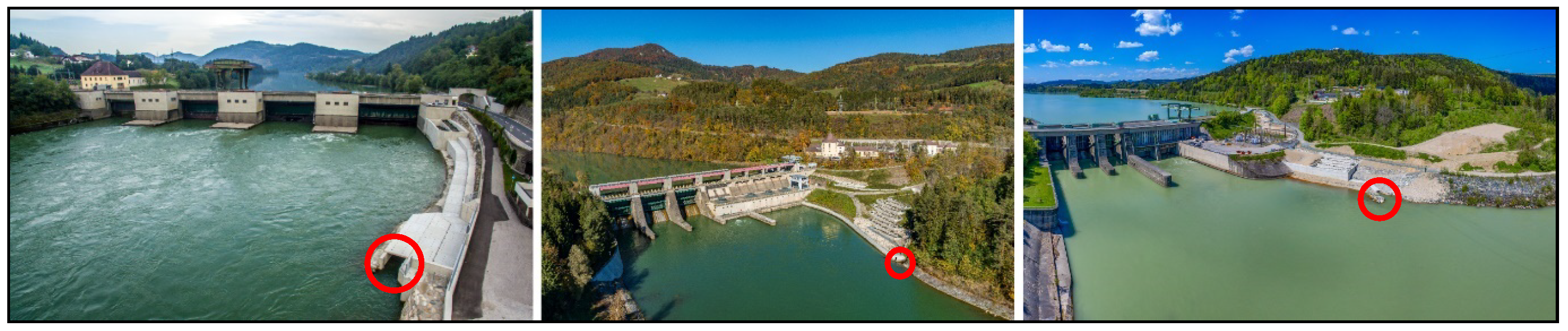
Funding

This research was funded by VERBUND Hydro Power GmbH, Europaplatz 2, A-1150 Vienna/Austria.

Institutional Review Board Statement

Not applicable.

Informed Consent Statement

Not applicable.

Data Availability Statement

Not applicable.

Conflicts of Interest

The authors declare no conflict of interest.

References

  1. Martinet, F.; Tödter, U.; Dubost, M. Die Letzten Naturnahen Alpenflüsse; CIPRA-Kleine Schriften; CIPRA: Vaduz, Liechtenstein, 1992. [Google Scholar]
  2. Waidbacher, H.; Haidvogl, G. Fish Migration and Fish Passage Facilites in the Danube: Past and Present. In Fish Migration and Fish Bypasses; Fishing News Books: Oxford, UK, 1998; pp. 85–98. [Google Scholar]
  3. Fehér, J.; Gaspar, J.; Veres, K.; Kiss, A.; Kristensen, P.; Künitzer, A.; Stein, U.; Austnes, K.; Spiteri, C.; Prins, T.; et al. Hydromorphological Alterations and Pressures in European Rivers, Lakes, Transitional and Coastal Waters. Thematic Assessment for EEA Water 2012; European Topic Centre on Inland, Coastal and Marine Waters: Prague, Czech, 2012. [Google Scholar]
  4. Arthington, A.H.; Welcomme, R.L. The Condition of Large River Systems of the World. Condition of the World´s Aquatic Habitats. World Fisheries Congress; Science Publishers: Lebanon, NH, USA, 1995; pp. 44–75. [Google Scholar]
  5. Poff, N.L.; Hart, D.D. How Dams Vary and Why It Matters for the Emerging Science of Dam Removal: An Ecological Classification of Dams Is Needed to Characterize How the Tremendous Variation in the Size, Operational Mode, Age, and Number of Dams in a River Basin Influences the Potential for Restoring Regulated Rivers via Dam Removal. Bioscience 2002, 52, 659–668. [Google Scholar] [CrossRef] [Green Version]
  6. Nilsson, C.; Reidy, C.A.; Dynesius, M.; Revenga, C. Fragmentation and Flow Regulation of the World’s Large River Systems. Science 2005, 308, 405–408. [Google Scholar] [CrossRef] [PubMed] [Green Version]
  7. Thorncraft, G.; Harris, J. Fish Passage and Fishways in New South Wales—A Status Report; Cooperative Research Centre for Freshwater Ecology: Canberra, Australia, 2000. [Google Scholar]
  8. Dudgeon, D.; Arthington, A.H.; Gessner, M.O.; Kawabata, Z.-I.; Knowler, D.J.; Lévêque, C.; Naiman, R.J.; Prieur-Richard, A.-H.; Soto, D.; Stiassny, M.L.J.; et al. Freshwater Biodiversity: Importance, Threats, Status and Conservation Challenges. Biol. Rev. Camb. Philos. Soc. 2006, 81, 163–182. [Google Scholar] [CrossRef] [PubMed]
  9. Postel, S.; Richter, B.D. Rivers for Life: Managing Water for People and Nature; Island Press: Washington, DC, USA, 2003. [Google Scholar]
  10. BMLFUW (Austrian Federal Ministry of Agriculture, Forestry, Environment and Water Management). Nationaler Gewässerbewirtschaftungsplan 2009; BMLFUW: Vienna, Austria, 2010; p. 225. [Google Scholar]
  11. Dumont, U.; Anderer, P.; Schwevers, U. Handbuch Querbauwerke; Ministerium für Umwelt und Naturschutz, Landwirtschaft und Verbraucherschutz des Landes Nordrhein-Westfalen: Düsseldorf, Germany, 2005. [Google Scholar]
  12. BMLFUW. Austrian Guidelines for Building Fishpasses (FP); The Austrian Federal Ministry of Agriculture, Forestry, Environment and Water Management: Vienna, Austria, 2012. [Google Scholar]
  13. Merkblatt DWA-M 509. Fischaufstiegsanlagen Und Fischpassierbare Bauwerke—Gestaltung, Bemessung, Qualitätssicherung, 1st ed.; Deutsche Vereinigung für Wasserwirtschaft, Abwasser und Abfall: Hennef, Germany, 2014. [Google Scholar]
  14. Seifert, K. Fischaufstiegsanlagen in Bayern Fischaufstiegsanlagen in Bayern; Landesfischereiverband Bayern e.V. und Bayrisches Landesamt für Umwelt: Augsburg, Germany, 2012. [Google Scholar]
  15. GOI. Guidelines for Maintaining Longitudinal Connectivity Trough Dams; Government of India, Central Water Commission: New Delhi, India, 2017. [Google Scholar]
  16. Mader, H.; Brandl, A.; Käfer, S. Design and Function Monitoring of an Enature® Vertical Slot Fish Pass in a Large Potamal River in Carinthia/Austria. Water 2020, 12, 551. [Google Scholar] [CrossRef] [Green Version]
  17. Gerhard, P. Die Fischwege. In Handbuch der Ingenieurwissenschaften; Wilhelm Engelmann: Leipzig, Germany, 1912; pp. 454–499. [Google Scholar]
  18. Brant, C.O.; Li, K.; Johnson, N.S.; Li, W. A Pheromone Outweighs Temperature in Influencing Migration of Sea Lamprey. R. Soc. Open Sci. 2015, 2, 150009. [Google Scholar] [CrossRef] [Green Version]
  19. Vetter, B.J.; Cupp, A.R.; Fredricks, K.T.; Gaikowski, M.P.; Mensinger, A.F. Acoustical Deterrence of Silver Carp (Hypophthalmichthys molitrix). Biol. Invasions 2015, 17, 3383–3392. [Google Scholar] [CrossRef]
  20. Amoser, S.; Ladich, F. Are Hearing Sensitivities of Freshwater Fish Adapted to the Ambient Noise in Their Habitats? J. Exp. Biol. 2005, 208 Pt 18, 3533–3542. [Google Scholar] [CrossRef] [Green Version]
  21. Benjamin, J.R.; Vidergar, D.T.; Dunham, J.B. Thermal Heterogeneity, Migration, and Consequences for Spawning Potential of Female Bull Trout in a River–Reservoir System. Ecol. Evol. 2020, 10, 4128–4142. [Google Scholar] [CrossRef] [Green Version]
  22. Pavlov, D.S. Structures Assisting the Migrations of Non-Salmonid Fish; Food & Agriculture Organization of the United Nations (FAO): Rome, Italy, 1990. [Google Scholar]
  23. Adam, B.; Lehmann, B. Ethohydraulik: Grundlagen, Methoden und Erkenntnisse; Springer: Berlin, Germany, 2011. [Google Scholar] [CrossRef]
  24. Larinier, M.; Travade, F.; Porcher, J.P. Fishways: Biological Basis, Design Criteria, and Monitoring; Conseil Superieur de la Peche; Food and Agriculture Organization of the United Nations: Rome, Italy, 2002. [Google Scholar]
  25. Brodersen, J.; Nicolle, A.; Nilsson, P.A.; Skov, C.; Brönmark, C.; Hansson, L.-A. Interplay between Temperature, Fish Partial Migration and Trophic Dynamics. Oikos 2011, 120, 1838–1846. [Google Scholar] [CrossRef]
  26. Fürst, J.; Kling, H.; Hörhan, T.; Nachtnebel, H.P. Hydro-Electric Power Plants (Map Sheet 9.1). In Hydrological Atlas of Austria; BMLFUW: Vienna, Austria, 2003. [Google Scholar]
  27. Haunschmid, R.; Schotzko, N.; Petz-Glechner, R.; Honsig-Erlenburg, W.; Schmutz, S.; Spindler, T.; Unfer, G.; Wolfram, G.; Bammer, V.; Hundritsch, L.; et al. Leitfaden zur Erhebung der Biologischen Qualitätselemente, Teil A1—Fische; BMLFUW: Vienna, Austria, 2010. [Google Scholar]
  28. Nilsson, C.; Polvi, L.E.; Lind, L. Extreme Events in Streams and Rivers in Arctic and Subarctic Regions in an Uncertain Future. Freshw. Biol. 2015, 60, 2535–2546. [Google Scholar] [CrossRef]
  29. Chiu, S.; Abrahams, M.V. Effects of Turbidity and Risk of Predation on Habitat Selection Decisions by Fathead Minnow (Pimephales promelas). Environ. Biol. Fishes 2010, 87, 309–316. [Google Scholar] [CrossRef]
  30. Brandl, A.; Käfer, S.; Fillitz, B.; Pinter, G.; Laaha, G.; Mader, H. Relevanz von Schlüsselreizen, Im Besonderen Licht Und Akustik, Zur Auffindbarkeit von Fischaufstiegen. Osterr. Wasser Abfallwirtsch. 2020, 72, 187–201. [Google Scholar] [CrossRef]
  31. Reichmann, M. Monitoring OWH Drau. Fischökologische Begleituntersuchungen—Bestands- und Migrationspotentialerhebungen; Endbericht: Klagenfurt, Austria, 2018. [Google Scholar]
  32. Mader, H.; Kratzert, F.; Käfer, S. FishCam—Videomonitoring Zur Funktionsanalyse von Fischaufstiegsanlagen. Wasserwirtschaft 2017, 107, 59–64. [Google Scholar] [CrossRef]
  33. Kratzert, F.; Mader, H. Advances of FishNet towards a Fully Automatic Monitoring System for Fish Migration. In EGU General Assembly Conference Abstracts; EGU: Vienna, Austria, 2017; p. 7932. [Google Scholar]
  34. Schiemer, F.; Waidbacher, H. Strategies for Conservation of a Danubian Fish Fauna. River Conserv. Manag. 1992, 62, 363–382. [Google Scholar] [CrossRef]
  35. Gelman, A.; Hill, J. Data Analysis Using Regression and Multilevel/Hierarchical Models; Cambridge University Press: Cambridge, UK, 2006. [Google Scholar] [CrossRef]
  36. Bates, D.; Kliegl, R.; Vasishth, S.; Baayen, H. Parsimonious Mixed Models. arXiv 2015, arXiv:1506.04967. [Google Scholar]
  37. Bates, D.; Mächler, M.; Bolker, B.; Walker, S. Fitting Linear Mixed-Effects Models Using lme4. J. Stat. Softw. 2015, 67, 1–48. [Google Scholar] [CrossRef]
  38. Cameron, C.; Trivedi, P. Regression Analysis of Count Data (Econometric Society Monographs); Cambridge University Press: Cambridge, UK, 1998; pp. 96–137. [Google Scholar] [CrossRef]
  39. Nelder, J.A.; Wedderburn, R.W.M. Generalized Linear Models. J. R. Stat. Soc. Ser. A 1972, 135, 370–384. [Google Scholar] [CrossRef]
  40. Dunn, P.K.; Smyth, G.K. Randomized Quantile Residuals. J. Comput. Graph. Stat. 1996, 5, 236–244. [Google Scholar] [CrossRef]
  41. Bürkner, P.-C. Brms: An R Package for Bayesian Multilevel Models Using Stan. J. Stat. Softw. 2017, 80, 1–28. [Google Scholar] [CrossRef] [Green Version]
  42. Vehtari, A.; Gelman, A.; Simpson, D.; Carpenter, B.; Bürkner, P.-C. Rank-Normalization, Folding, and Localization: An Improved Rhat for Assessing Convergence of MCMC (with Discussion). Bayesian Anal. 2021, 16, 667–718. [Google Scholar] [CrossRef]
  43. Mader, H. What’s Luring Fish into Bypass Systems? In A Monitoring Project at Nature Like Bypass Channels in Potamal Fish Region. In Proceedings of the Hidroenergia 2008, Bled, Slovenia, 11–13 June 2008; Hidroenergia 2008 Proceedings (CD). ESHA: Brüssel, Belgium, 2008; pp. 1–8. [Google Scholar]
  44. Brandl, A.; Käfer, S.; Laaha, G. Temperatur Als Schlüsselreiz Für Die Auffindbarkeit von Fischaufstiegsanlagen. Wasserwirtschaft 2022, 12–18. [Google Scholar] [CrossRef]
  45. Caudill, C.C.; Keefer, M.L.; Clabough, T.S.; Naughton, G.P.; Burke, B.J.; Peery, C.A. Indirect Effects of Impoundment on Migrating Fish: Temperature Gradients in Fish Ladders Slow Dam Passage by Adult Chinook Salmon and Steelhead. PLoS ONE 2014, 8, e85586. [Google Scholar] [CrossRef] [PubMed]
  46. Kubecka, J.; Duncan, A. Diurnal Changes of Fish Behaviour in a Lowland River Monitored by a Dual-Beam Echosounder. Fish. Res. 1998, 35, 55–63. [Google Scholar] [CrossRef]
  47. Lelek, A.; Libosvárský, J. Výskyt Ryb v Rybím Přechodu Na Řece Dyji Při Břeclavi [The Occurrence of Fish in a Fish Ladder in Dyje River near Břeclav]. Folia Zool. 1960, 9, 293–308. [Google Scholar]
  48. Rakowitz, G.; Berger, B.; Kubečka, J.; Keckeis, H. Functional Role of Environmental Stimuli for the Spawning Migration in Danube Nase Chondrostoma Nasus (L.). Ecol. Freshw. Fish. 2008, 17, 502–514. [Google Scholar] [CrossRef]
  49. Prchalová, M.; Horký, P.; SlavíK, O.; VetešNíK, L.; Halačka, K. Fish Occurrence in the Fishpass on the Lowland Section of the River Elbe, Czech Republic, with Respect to Water Temperature, Water Flow and Fish Size. Folia Zool. 2011, 60, 104–114. [Google Scholar] [CrossRef]
  50. Lilja, J.; Keskinen, T.; Marjomäki, T.J.; Valkeajärvi, P.; Karjalainen, J. Upstream Migration Activity of Cyprinids and Percids in a Channel, Monitored by a Horizontal Split-Beam Echosounder. Aquat. Living Resour. 2003, 16, 185–190. [Google Scholar] [CrossRef]
  51. Jonsson, N. Influence of Water Flow, Water Temperature and Light on Fish Migrations in Rivers. Nord. J. Freshw. Res 1991, 66, 20–35. [Google Scholar]
  52. Winter, H.V. Fishway Efficiency, Delay and Passage Behaviour of Ide in Relation to Attraction Flow. A Fisheye View on Fishways. Ph.D. Thesis, Wageningen University, Wageningen, The Netherlands, 2007; p. 196. [Google Scholar]
  53. Geeraerts, C.; Ovidio, M.; Verbiest, H.; Buysse, D.; Coeck, J.; Belpaire, C.; Philippart, J. Mobility of Individual Roach Rutilus Rutilus (L.) in Three Weir-Fragmented Belgian Rivers. Hydrobiologia 2007, 582, 143–153. [Google Scholar] [CrossRef]
  54. Lucas, M.C. The Influence of Environmental Factors on Movements of Lowland-River Fish in the Yorkshire Ouse System. Sci. Total Environ. 2000, 251–252, 223–232. [Google Scholar] [CrossRef]
  55. Kotusz, J.; Witkowski, A.; Baran, M.; Błachuta, J. Fish Migrations in a Large Lowland River (Odra R., Poland)—Based on Fish Pass Observations. Folia Zool. Praha. 2006, 55, 386–398. [Google Scholar]
  56. Larinier, M. Location of Fishways. BFPP Bull. Fr. Pech. Prot. Milieux Aquat. 2002, 364, 39–53. [Google Scholar] [CrossRef] [Green Version]
  57. Mader, H.; Bogner, K. Attraction Flow at the Entrance of Bypass-Channels [Lockströmung Bei Naturnahen Umgehungsgerinnen Im Potamal]. Wasserwirtschaft 2001, 91, 194–199. [Google Scholar]
  58. Grünzner, M.; Haimerl, G. Numerical Simulation Downstream Attraction Flow at Danube Weir Donauwrth. In Proceedings of the 9th International Symphosium on Ecohydraulics, Vienna, Austria, 17–21 September 2012; ISBN 978-3-200-02862-3. [Google Scholar]
  59. Mader, H.; Kraml, J.; Lebiedzinski, K.; Käfer, S.; Mayr, P. Modelling and Monitoring Results of Fish Migration into Fishpasses vs. Attraction Flow. In In Proceedings of the 10th International Symposium on Ecohydraulics, Trondheim, Norway, 23–27 June 2014. [Google Scholar]
  60. Li, G.; Sun, S.; Liu, H.; Zheng, T. Optimizing the Entrance Location for a Fish Pass Facility with Limited Attraction Flow in a Large River—A Case Study of the Jinsha River, China. Can. J. Civ. Eng. 2019, 46, 847–857. [Google Scholar] [CrossRef]
  61. Nunn, A.; Copp, G.; Vilizzi, L.; Carter, M. Seasonal and Diel Patterns in the Migrations of Fishes between a River and a Floodplain Tributary. Ecol. Freshw. Fish 2010, 19, 153–162. [Google Scholar] [CrossRef]
  62. Baumgartner, L.J.; Stuart, I.G.; Zampatti, B.P. Determining Diel Variation in Fish Assemblages Downstream of Three Weirs in a Regulated Lowland River. J. Fish Biol. 2008, 72, 218–232. [Google Scholar] [CrossRef]
  63. Keep, J.K.; Watson, J.R.; Cramp, R.L.; Jones, M.J.; Gordos, M.A.; Ward, P.; Franklin, C.E. Low Light Levels Increase Avoidance Behaviour of Diurnal Fish Species: Implications for Road Culverts. bioRxiv 2020. [Google Scholar] [CrossRef] [Green Version]
  64. Perkin, E.K.; Hölker, F.; Richardson, J.S.; Sadler, J.P.; Wolter, C.; Tockner, K. The Influence of Artificial Light on Stream and Riparian Ecosystems: Questions, Challenges, and Perspectives. Ecosphere 2011, 2, art122. [Google Scholar] [CrossRef]
  65. McKibben, J.R.; Bass, A.H. Behavioral Assessment of Acoustic Parameters Relevant to Signal Recognition and Preference in a Vocal Fish. J. Acoust. Soc. Am. 1998, 104, 3520–3533. [Google Scholar] [CrossRef]
  66. Kaatz, I.M.; Lobel, P.S. Acoustic Behavior and Reproduction in Five Species of Corydoras Catfishes (Callichthyidae). Biol. Bull. 1999, 197, 241–242. [Google Scholar] [CrossRef]
  67. Enger, P.S.; Karlsen, H.E.; Knudsen, F.R.; Sand, O. Detection and Reaction of Fish to Infrasound. ICES Mar. Sei. Symp. 1993, 196, 108–112. [Google Scholar]
Figure 1. Study sites: Hydro Power Plants (HPP) Lavamünd (left), Schwabeck (middle) and Edling (right), situated at river Drava, Carinthia/Austria. Red circles indicate the entrances of the fish passes.
Water 14 01530 g001
Figure 2. Austrian part of the river Drava with sites of the HPP, red squares indicate the runoff-river-stations with hydropeaking according to [26], © Land Kärnten—KAGIS, BEV.
Water 14 01530 g002
Figure 3. Entrance area fish pass of Edling with LED stripes and speakers.
Water 14 01530 g003
Figure 4. Means and variances of ascent rates across the different years; boxes indicate the inter-quartile range (IQR), black horizontal lines within the boxes show the median, whiskers show values within 1.5 × IQR anddots indicate outliers.
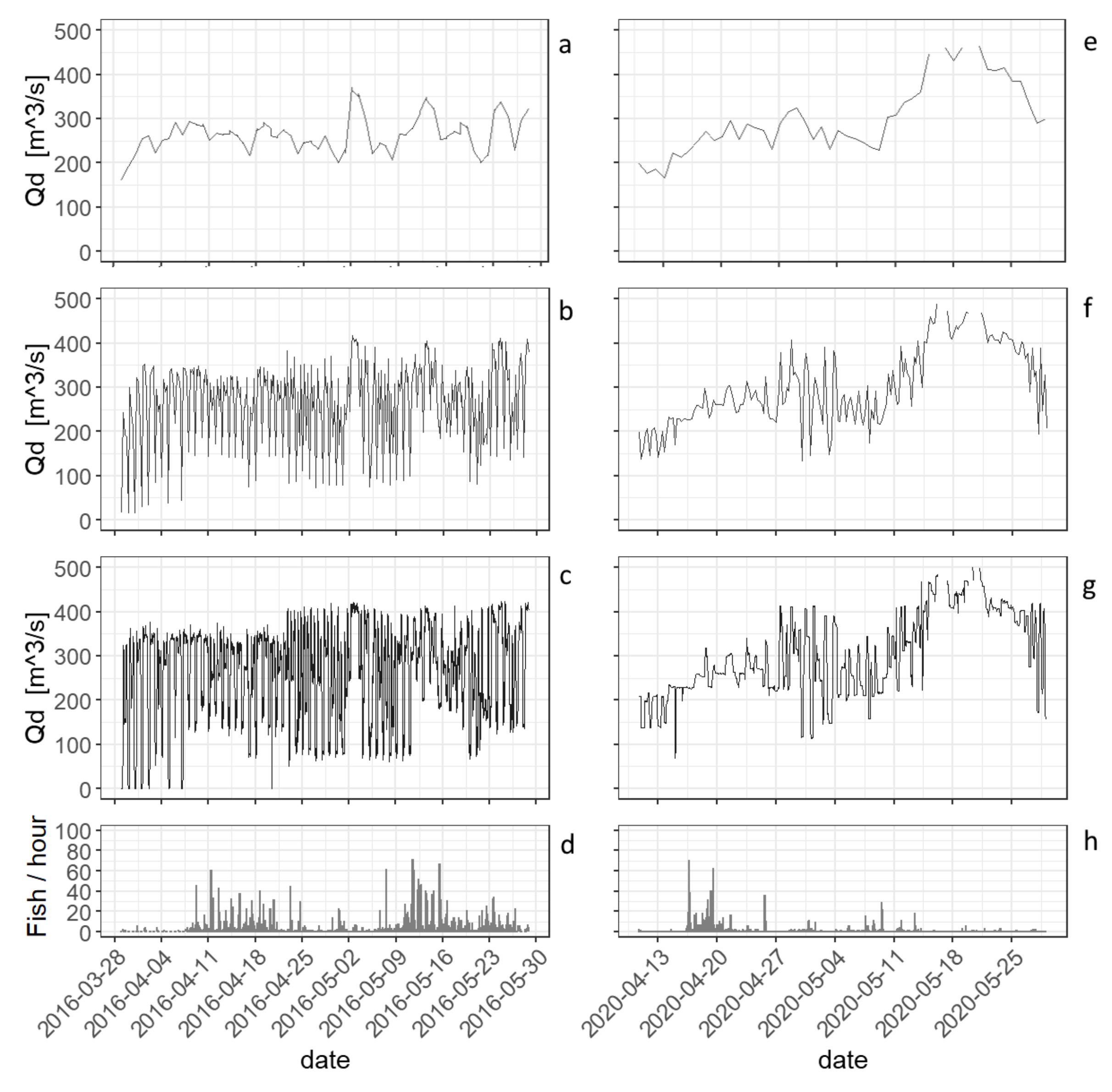
Water 14 01530 g004
Figure 5. Diurnal variation of the discharge of the Drava at the HPP Lavamünd for different time intervals ((a,e): 24-h data; (b,f): 6-h data; (c,g): 1-h data) with ascent rates; ((d,h): 1-h data).
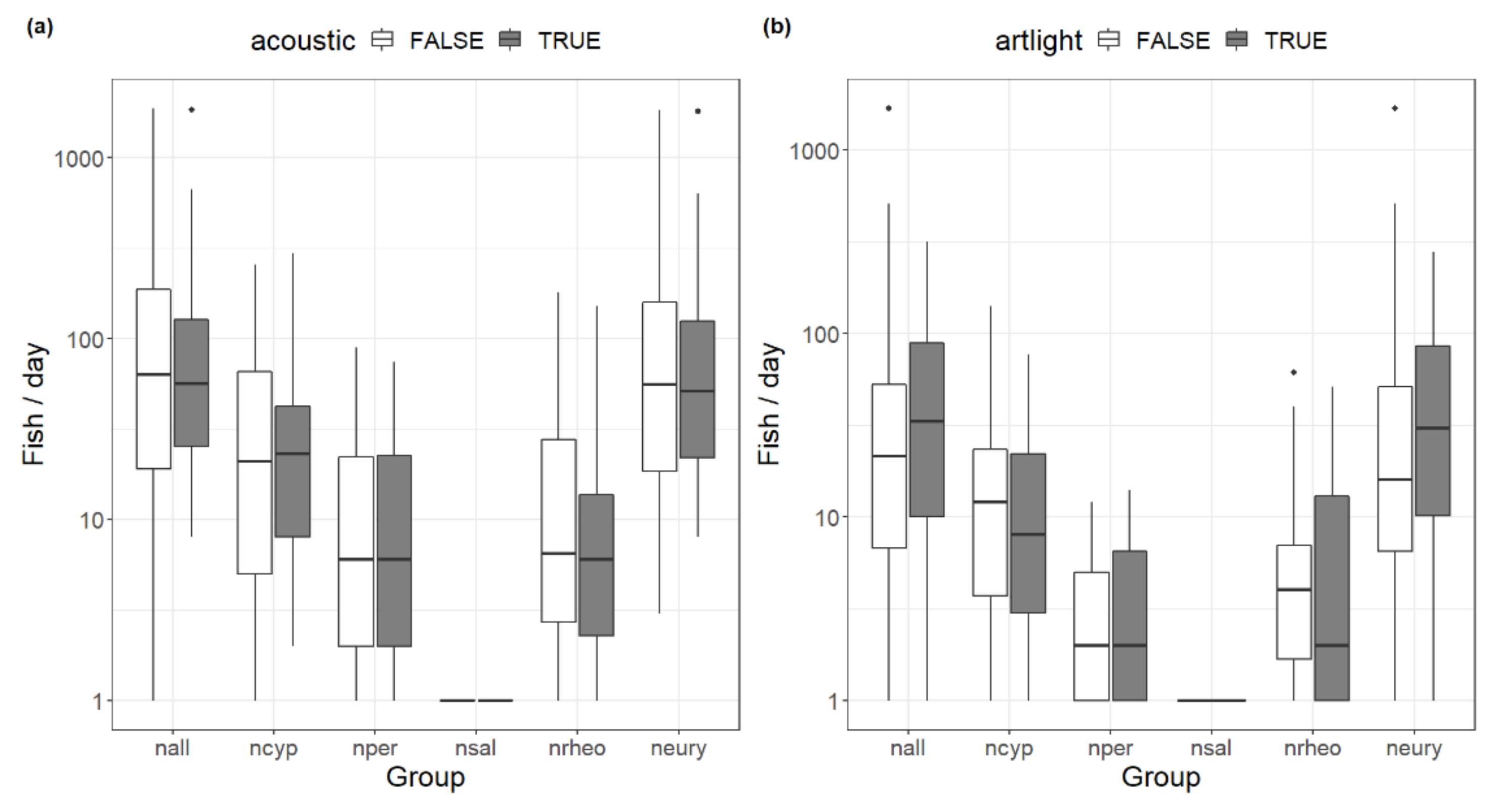
Water 14 01530 g005
Figure 6. Boxplots of artificial stimuli acoustic (a) and light (b), at the fish pass of HPP Edling sorted by investigated groups; boxes indicate the inter-quartile range (IQR), black horizontal line within the boxes show the medians, whiskers show values within 1.5 × IQR and dots indicate outliers.
Water 14 01530 g006
Table 1. Overview of the fish passes at the three study sites, Lavamünd, Schwabeck and Edling, situated at river Drava, Carinthia/Austria.
LavamündSchwabeckEdling
Total drop height10 m20 m22 m
Total no. of pools74158148
No. of resting pools142224
Drop height btw. pools13 cm13 cm13 cm
Pool dimension (l × w)3.0 m × 2.2 m3.0 m × 2.2 m3.0 m × 2.2 m
Slot width40 cm40 cm40 cm
Total length300 m550 m650 m
Distance to obstacle110 m120 m150 m
Table 2. Monitoring periods at the study sites Lavamünd, Schwabeck and Edling.
LavamündSchwabeckEdling
Period 126 August–5 December 20158 April–26 May 20169 April–18 June 2019
Period 229 March–8 November 20165 July–9 September 201617 September–4 November 2019
Period 3 3 October–6 December 201610 April–23 June 2020
Period 4 21 March–9 June 2017
Table 3. Specification of the temperature sensors for recording the water temperature at all three study sites.
HOBO U22 Specifications
Operation range−40 °C to 50 °C in water
Accuracy±0.21 °C from 0 °C to 50 °C
Resolution0.02 °C at 25 °C
Response time 5 min in water
WaterproofTo 120 m
Table 4. Weekly pattern of the artificial key stimuli of light and acoustics at the fish pass at HPP Edling.
Day of WeekStimulusDay of WeekStimulus
MondayAcousticsThursdayAcoustics
TuesdayLightFridayLight
Wednesday-Saturday/Sunday-
Table 5. Observed numbers of fish species from FishCam recording (count and percent of total) and their occurrence according to the Natural guideline and electrofishing downstream from the study area. [27].
SpeciesFishCamGuidelineDownstreamPercentSpeciesFishCamGuidelineDownstreamPercent
Alburnus alburnus23,095tt57.46Leuciscus aspius3 0.01
Alburnoides bipunctatus4918tt12.24Salvelinus fontinalis2 0
Rutilus rutilus3299tt8.21Barbatula barbatula2r 0
Perca fluviatilis3018tt7.51Leuciscus idus2 0
Chondrostoma nasus1414ll3.52Gymnocephalus schraetser2 0
Abramis brama1065tt2.65Lepomis gibbosus2 0
Squalius cephalus816ll2.03Anguilla anguilla1 0
Blicca bjoerkna599 1.49Rutilus pigus1 0
Unknown356 0.89Carassius carassius1r 0
Cyprinidae unknown286 0.71Sander lucioperca1 0
Gobio gobio211tt0.52Ballerus sapa1 0
Leuciscus leuciscus193t 0.48Hucho hucho0l -
Oncorhynchus mykiss185 0.46Telestes souffia0t -
Salmonidae unknown179 0.45Romanogobio kesslerii0r -
Scardinius erythroph.168r 0.42Vimba vimba0r -
Barbus barbus67ll0.17Alburnus mento0r -
Salmo trutta fario57rr0.14Barbus balcanicus0r -
Thymallus thymallus47t 0.12Cobitis elongatoides0r -
Esox lucius45tt0.11Acipenser ruthenus0r -
Salmo trutta lacustris42 0.1Zingel streber0r -
Gymnocephalus cernua30 0.07Romanogobio vladykovi0r -
Cottus gobio28r 0.07Zingel zingel0r -
Silurus glanis13t 0.03TOTAL no. observed40,194
Carassius gibelio12 0.03
Tinca tinca11r 0.03Lead species (l)343
Lota lota10tt0.02Typical species (t)12138
Eudontomyzon mariae8t 0.02Rare species (r)7161
Cyprinus carpio4r 0.01Not mentioned (-)14--
Table 6. Predictor variables for the statistical analyses with survey intervals and study site.
VariableSurvey IntervalHPP Site
Drava discharge (Qd)15 minAll sites
Fishpass discharge (Qf)15 minAll sites
Guiding flow (Qa)15 minAll sites
Season-adjusted watertemp. (tres)1 hAll sites
Watertemperature difference fish pass/Drava (tdiff)1 hAll sites
Season (seas.)-All sites
Study location (Site)-All sites
Year-All sites
Artificial light1 dayEdling
Acoustic1 dayEdling
Table 7. Statistical summary over the independent variable discharges fish passes (Qf), discharge Drava (Qd), attraction flow (Qa), residuals of the water temperature Drava (tres), difference in water temperature fish passes–Drava (tdiff) and ascent rate of all observed fish (nall)—1-h data.
Qf [m3/s]Qd [m3/s]Qa [%]tres [°C]tdiff [°C]nall [-]
Min.0.080.10.025−5.32−2.380
Mean0.38274.24.660.160.0962.18
Median0.40278.50.140.380.0010
Max.0.49932.84415.083.64981
SD0.059140.43324.9841.7680.41015.51
Table 8. Regression models for the group of all individuals, 1-h data and 24-h data with incident rate ratios (IRR), confidence intervals (CI) for the frequentist models and credibility intervals (CI) for the Bayesian models. Glmm = frequentist approach, brm = Bayesian approach, Qd = discharge Drava, Qf = discharge fish pass, Qa = attraction flow, tres = residuals of the water temperature and tdiff = difference in water temperature btw. Fish pass and Drava, SB = Schwabeck and ED = Edling; p-values < 0.05 indicating significant parameters.
All Fish1-h Glmm1-h Brm24-h Glmm24-h Brm
PredictorsIRRCI (95%)p-ValueIRRCI (95%)IRRCI (95%)p-ValueIRRCI (95%)
(Intercept)0.360.09–1.390.1370.290.03–2.3930.933.96–241.850.00119.030.41–294.58
Qd0.990.97–1.000.0550.990.97–1.000.850.80–0.91<0.0010.850.80–0.91
Qf0.940.90–0.980.0030.940.90–0.980.930.80–1.090.3710.920.79–1.08
Qa10.99–1.00<0.00110.99–1.000.580.01–26.480.7810.740.02–40.05
tres1.631.57–1.69<0.0011.631.57–1.691.481.34–1.63<0.0011.491.35–1.65
tdiff2.972.61–3.39<0.0012.962.60–3.391.691.03–2.780.041.651.01–2.66
Site: SB1.891.61–2.23<0.0011.91.62–2.241.81.12–2.890.0141.811.14–2.93
Site: ED3.880.51–29.180.1884.170.07–218.606.470.80–52.460.088.430.15–980.87
Seas.: Spring3.593.07–4.19<0.0013.593.09–4.215.123.38–7.77<0.0015.323.52–8.13
Seas.: Summer1.941.65–2.29<0.0011.941.65–2.303.922.52–6.09<0.0014.022.58–6.32
Seas.: Winter0.040.01–0.09<0.0010.030.01–0.080.040.01–0.16<0.0010.040.01–0.18
Ran. Eff.
SD Intercept1.26 1.94 1.30 2.04
Observations18,45618,456775775
Table 9. Regression models for the flow preference guilds rheophilic (rheo.) and eurytopic w/o Bream (eury.). Side by side, 1-h data and 24-h data, frequentist models and all study sites.
Rheo. 1-h GlmmEury. 1-h GlmmRheo. 24-h GlmmEury. 24-h Glmm
PredictorsIRRCI (95%)p-ValueIRRCI (95%)p-ValueIRRCI (95%)p-ValueIRRCI (95%)p-Value
(Intercept)0.390.10–1.620.1950.090.03–0.30<0.00120.51.66–253.380.0195.710.88–36.850.067
Qd0.950.93–0.97<0.0010.980.97–1.000.0260.820.76–0.89<0.0010.850.80–0.90<0.001
Qf0.970.91–1.040.4240.910.87–0.95<0.00110.81–1.230.9790.980.85–1.120.72
Qa0.980.97–0.98<0.00111.00–1.000.0430.990.01–68.330.9960.020.00–0.690.03
tres1.381.29–1.47<0.0011.821.75–1.89<0.0011.21.06–1.370.0051.771.63–1.92<0.001
tdiff1.41.15–1.700.0012.492.19–2.84<0.0010.790.46–1.330.372.31.47–3.59<0.001
Site: SB0.710.53–0.950.021.431.19–1.71<0.0010.690.36–1.300.2451.490.94–2.340.088
Site: ED0.890.14–5.490.99.121.48–56.120.0171.770.36–8.570.48110.721.58–72.600.015
Seas.: Spring2.852.24–3.63<0.0011.881.63–2.17<0.0013.352.17–5.17<0.0012.972.08–4.23<0.001
Seas.: Summer0.650.50–0.830.0011.771.49–2.10<0.0011.120.70–1.790.6443.292.18–4.96<0.001
Seas.: Winter0.080.03–0.23<0.0010.030.00–0.21<0.0010.060.01–0.27<0.0010.030.00–0.280.002
Ran. Eff.
SD Intercept1.01 1.020.67 1.09
Observations18,45618,456775775
Table 10. Regression models for the families Salmonidae (sal.), Cyprinidae (cyp.) and Percidae (perc.); 1-h data and all study sites.
Sal. 1-h GlmmCyp. 1-h GlmmPerc. 1-h Glmm
PredictorsIRRCI (95%)p-ValueIRRCI (95%)p-ValueIRRCI (95%)p-Value
(Intercept)00.00–0.01<0.0010.360.11–1.170.090.050.01–0.310.001
Qd0.990.97–1.020.5770.960.94–0.98<0.0011.010.99–1.040.165
Qf1.081.00–1.170.0590.950.90–1.000.060.880.83–0.93<0.001
Qa0.980.97–0.99<0.0010.990.99–0.99<0.00110.99–1.000.044
tres1.311.21–1.43<0.0011.471.41–1.54<0.0012.192.04–2.35<0.001
tdiff0.870.61–1.250.4651.531.32–1.78<0.0012.582.13–3.13<0.001
Site: SB6.84.71–9.81<0.0010.670.54–0.84<0.0011.561.21–2.020.001
Site: ED1.260.53–3.020.6023.020.61–15.040.1785.270.41–68.270.204
Seas.: Spring1.090.79–1.510.6063.743.13–4.46<0.0010.390.32–0.49<0.001
Seas.: Summer1.551.12–2.150.0080.870.72–1.070.1841.51.18–1.910.001
Seas.: Winter0.290.07–1.250.0960.040.01–0.14<0.00100.00–Inf0.988
Ran. Eff.
SD Intercept0.170.792.02
Observations18,45618,45618,456
Table 11. Regression models for the families Salmonidae (sal.), Cyprinidae (cyp.) and Percidae (per.); 24-h data and all study sites.
Sal. 24-h GlmmCyp. 24-h GlmmPerc. 24-h Glmm
PredictorsIRRCI (95%)p-ValueIRRCI (95%)p-ValueIRRCI (95%)p-Value
(Intercept)1.360.24–7.840.7275.060.52–48.910.1624.60.38–55.150.229
Qd0.840.77–0.92<0.0010.820.76–0.89<0.0010.90.83–0.970.008
Qf1.040.88–1.220.6561.10.91–1.330.3180.870.74–1.040.128
Qa00.00–0.100.0020.760.01–51.620.8990.080.00–4.840.226
tres1.331.20–1.48<0.0011.331.19–1.48<0.0012.121.88–2.39<0.001
tdiff1.460.72–2.970.2990.660.40–1.080.0953.611.87–6.95<0.001
Site: SB4.882.90–8.20<0.0010.870.49–1.540.631.670.94–2.970.079
Site: ED0.970.43–2.210.9467.961.51–41.970.0144.950.38–65.040.224
Seas.: Spring1.30.88–1.900.1855.233.45–7.90<0.0010.550.35–0.880.012
Seas.: Summer2.261.46–3.49<0.0011.470.92–2.330.1032.761.71–4.47<0.001
Seas.: Winter0.270.05–1.360.1130.030.01–0.17<0.00100.00–Inf0.995
Ran. Eff.
SD Intercept0.080.771.95
Observations775775775
Table 12. Regression models for the species Bleak (Alburnus alburnus), Nase (Chondrostoma nasus), Bream (Abramis brama) and Chub (Squalius cephalus); 1-h data and all study sites.
Bleak 1-h GlmmNase 1-h GlmmBream1-h GlmmChub 1-h Glmm
PredictorsIRRCIp-ValueIRRCIp-ValueIRRCIp-ValueIRRCIp-Value
(Intercept)0.110.02–0.670.0160.640.01–52.160.84200.00–0.03<0.0010.020.01–0.09<0.001
Qd0.990.97–1.020.5390.620.53–0.74<0.0010.930.90–0.96<0.0010.950.92–0.990.004
Qf0.880.82–0.93<0.0011.190.90–1.570.2280.930.85–1.030.1490.940.84–1.050.245
Qa11.00–1.010.49200.00–0.00<0.00110.99–1.000.410.980.97–0.990.002
tres1.761.65–1.87<0.0011.741.34–2.26<0.0011.351.23–1.48<0.0011.381.25–1.52<0.001
tdiff4.763.74–6.06<0.0017.223.25–16.05<0.0013.592.73–4.72<0.0012.071.51–2.84<0.001
Site: SB2.662.05–3.44<0.0010.050.02–0.14<0.0012.911.84–4.61<0.0011.050.64–1.730.845
Site: ED7.120.54–93.320.1350.010.00–1.550.07127.41.37–5490.031.850.75–4.550.181
Seas.: Spring6.194.65–8.23<0.00133.4213.88–80.46<0.0014.243.02–5.95<0.0015.493.76–8.02<0.001
Seas.: Summer4.43.28–5.90<0.0011.280.45–3.590.6452.341.46–3.76<0.0012.431.50–3.93<0.001
Seas.: Winter00.00–Inf0.98511.271.21–104.880.03300.00–Inf0.99300.00–Inf0.993
Ran. Eff.
SD Intercept2.04 7.38 2.70 0.20
Observations18,45618,45618,45618,456
Table 13. Regression models for the species Bleak (Alburnus alburnus), Nase (Chondrostoma nasus), Bream (Abramis brama) and Chub (Squalius cephalus); 24-h data and all study sites.
Bleak 24-h GlmmNase 24-h GlmmBream 24-h GlmmChub 24-h Glmm
PredictorsIRRCIp-ValueIRRCIp-ValueIRRCIp-ValueIRRCIp-Value
(Intercept)33.881.72–667.090.0212513.70.20–3×1060.1030.330.01–17.040.580.570.08–4.320.588
Qd0.860.78–0.960.0070.440.25–0.790.0050.750.66–0.87<0.0011.020.95–1.100.567
Qf0.760.59–0.980.0341.090.58–2.060.791.040.77–1.390.8180.880.74–1.050.168
Qa0.980.00–5190.99400.00–0.470.04400.00–2.290.0839.650.15–6130.285
tres1.591.35–1.86<0.0011.660.97–2.840.0661.331.14–1.55<0.0011.191.07–1.330.001
tdiff2.651.14–6.200.024505.696.90–3×1030.0043.311.62–6.780.0011.340.90–1.980.146
Site: SB1.990.95–4.160.0680.040.01–0.23<0.0012.841.10–7.370.0320.960.51–1.800.905
Site: ED11.170.81–1530.07100.00–0.130.00933.911.31–8810.0342.641.23–5.660.013
Seas.: Spring9.274.46–19.25<0.00159.019.76–356.75<0.0017.453.95–14.03<0.0013.492.26–5.42<0.001
Seas.: Summer9.44.38–20.21<0.0016.410.65–62.910.1116.52.91–14.50<0.0011.770.99–3.150.053
Seas.: Winter00.00–Inf0.99315.40.39–605.600.14400.00–Inf0.99600.00–Inf0.996
Ran. Eff.
SD Intercept1.975.133.090.11
Observations775775775775
Publisher’s Note: MDPI stays neutral with regard to jurisdictional claims in published maps and institutional affiliations.

