Article

An Approach for Monitoring and Classifying Marshlands Using Multispectral Remote Sensing Imagery in Arid and Semi-Arid Regions

1
Institute of Environmental Sciences, Hungarian University of Agriculture and Life Sciences, Páter Károly u. 1., 2100 Gödöllő, Hungary
2
Collage of Engineering, University of Thi-Qar, Thi-Qar City 00964, Iraq
3
Faculty of Geo-Information Science and Earth Observation, University of Twente, Hengelosestraat 99, 7514 AE Enschede, The Netherlands
*
Author to whom correspondence should be addressed.
Water 2022, 14(10), 1523; https://doi.org/10.3390/w14101523
Submission received: 2 April 2022 / Revised: 30 April 2022 / Accepted: 4 May 2022 / Published: 10 May 2022

Abstract

:
Marshlands in arid and semi-arid areas are considered constantly changing environments due to unsecured water supplies as a result of high evapotranspiration and limited and highly variable rainfall. Classification of marshlands in these regions and mapping of their land cover is not an easy task and maps need to be upgraded frequently. Satellites provide enormous amounts of information and data for the continuous monitoring of changes. The aim of this paper is to introduce an approach using multispectral satellite imagery that was adopted to classify and monitor the Al Hammar Marsh (Iraq) over several years and to suggest a relationship between the Normalized Difference Vegetation Index (NDVI), the Normalized Difference Moisture Index (NDMI), and the Normalized Difference Water Index (NDWI), using Landsat 8 data with a resolution of 30 m × 30 m, validated with Sentinel-2 datasets at 10 m × 10 m. Six land cover classes were used: (1) open water, (2) dry area, (3) dense vegetation, (4) medium-density vegetation, (5) sparse vegetation, and (6) wet soil. Three indices, NDWI, NDMI, and NDVI, were chosen for the automatic classification of each pixel and the creation of a time series of land cover maps. The proposed method can efficiently classify and monitor marshlands and can be used to study different marshlands by adjusting the thresholds for NDVI, NDMI, and NDWI. Overall, the correlation for all classes (R) between Landsat 8 and Sentinel-2 is about 0.78. Thus, this approach will help to preserve marshes through improved water management.

1. Introduction

Large changes in land cover occur all around the world. These changes cause, among other things, many environmental problems, such as erosion and increased surface runoff, and are part of complex interactions with drought, climate, and biodiversity [1]. Information on land cover/land use (LCLU) is important on both large and small scales for understanding the influences of many environmental factors, such as climate change, desertification, and others [2].
Wetlands play an essential role in local and regional water cycles, especially in arid and semi-arid regions. They are considered to be natural water reservoirs, habitats for a large number of plants and animals, as well as carbon stores, and thus play a major role in reducing global warming [3]. Marshlands are some of the most complex ecosystems and include a large number of different habitat types (e.g., grasslands, aquatic and agricultural lands).
Due to major anthropogenic interventions within their catchments, many rivers that feed marshes in these areas undergo major changes in relation to land cover and land use over time. Many interventions are focused on controlling and altering the natural hydrology of these rivers and ultimately modifying the flooding regimes. The changes have negatively impacted marshlands both in terms of water availability and water quality. In efforts to capture the impact of the interventions on the marshes, the use of remote sensing data collected through the Landsat programme has become essential. Remote sensing data are optimal for covering the spatial extents of large marshlands [4] and monitoring their complex ecosystems. Regular mapping of land cover/land use systems is an ideal way to monitor the dynamics of wetland ecosystems [5].
During the past decades, remote sensing has become an effective tool for monitoring land cover changes. Remote sensing detects changes in land cover by detecting changes in the amount of radiation reflected from the surface. These changes in radiation are only partially caused by changes in land cover, as many other factors affect radiation, such as weather, soil moisture, and sun angles. The signals are mixed, so there is a continuous need to develop increasingly sensitive methods to monitor land cover changes [6].
A recent review conducted by Guo et al. [4] found that remote sensing is extensively used to assess wetlands across the globe, between 300 to 500 peer-reviewed articles being published annually over the past five years. Their results also highlighted the Landsat programme’s importance: out of the 5719 wetland research papers published globally, 1259 papers used Landsat data. In their study, satellite images taken by the Landsat 4, 5, 7, and 8 sensors provided a rich time series of their study area that spans over 31 years (1986–2017) [4].
Analysis of satellite imagery of a marsh environment is one of the established methodologies and is widely used in environmental planning processes in marsh areas that are at risk from local changes and changes in the sources of rivers [7]. Furthermore, Tucker and Compton [8] suggested a technique for deriving green biomass data from the Normalized Difference Vegetation Index (NDVI) [8]. Further analysis methods are Selective Principal Components Analysis and methods based on variance–covariance matrices [9]. According to Singh [6], direct multi-date classification is built upon linking a single test dataset with different dates to monitor land cover change. Post-classification analysis is applied to time series of classified spectral imagery to compare different time steps independently [6,10]. Lu, Mausel, and Batistella [10] applied a combination of image enhancement and post-classification for enhancing changes using a binary mask to indicate where change has occurred in different periods.
The above studies classified wetlands into basic classes: open water, vegetation, and bare soil. With more elaborate techniques, significantly more details can be extracted from the imagery [11]. In wetland monitoring, band ratio indices are favoured over single bands as predictor variables because band ratios eliminate noise [12,13].
A series of spectral indices were developed to assess the temporal variability of marshes’ inundated areas and the health of vegetation covers. The indices included the NDVI [14], which is based on the difference between the reflectance of the visible red (R) and near-infrared (NIR) bands. It is an indicator that can be used to analyse the strong chlorophyll absorption region of R and the high reflectance plateau of vegetation canopies in NIR. Healthy vegetation is indicated by high values, whereas bare soil has values near to zero and open water has values well below zero. This discrimination method allows the cover classification to be reduced to a level or density slicing operation [15] where threshold values are used to separate classes.
On the one hand, the traditional survey of wetlands is a fieldwork-intensive task, which is time-consuming and expensive; thus, it is usually suitable only for small areas [16]. On the other hand, remote sensing provides coverage at various scales and can be repeated over time; the monitoring is low-cost and high-efficiency [17]. Typically, the boundaries between wetland types are fuzzy since they change gradually from bare soil to wet soil to different vegetation covers or open water. Within vegetated areas, there are many different types with different densities of vegetation; therefore, the image parameters used for the monitoring have to be selected to fit the characteristics of the wetlands, and the analysis methods should also be chosen accordingly [18].
The Normalized Difference Moisture Index (NDMI) is derived from two infrared bands. It is sensitive to the moisture content of the vegetation, but it can also be used for separating the basic land cover classes of wetlands. The NDMI is the normalized difference between near-infrared (NIR) and short-wave infrared (SWIR) bands [19]. In the original publication, this index was referred to as NDWI. However, for the sake of differentiating it from the identically named index of McFeeters [20], in what follows, the widely accepted name Normalised Difference Moisture Index (NDMI) will be used.
Several techniques used wetness indices to group different vegetation classes and separate flooded and non-flooded pixels by monitoring dynamically changing inundation extents [21,22]. However, due to the complexity and variety of surface characteristics of wetlands, there is no single foolproof method for calculating evapotranspiration and these methods can only be successfully applied to wetlands with uniform vegetation cover [23].
The lack of availability of unsecured water in arid and semi-arid areas threatens the preservation of marshlands due to high levels of evapotranspiration and limited rainfall, dramatic changes making the classification and creation of land cover maps of wetlands a difficult task, yet one that is needed for continuous renewal. This paper introduces a fast and low-cost method for classifying and monitoring marshlands in these regions. The analysis is based on analysing water coverage with the NDWI and characterising vegetation with NDMI and NDVI indices. It is a modification of the UNEP methodology. The results can support wetland modelling, such as hydrodynamic models for the optimization of the distribution of available water to preserve marshes, and link this approach to wetland mapping for the calculation of spatial evaporation and transpiration.
The study area (the Al Hammar marsh in the southern part of Iraq) was chosen because this marsh was exposed to extreme desiccation in the 1990s. The availability and regime of water inflow have changed due to major anthropogenic interventions in the last several decades. Further, they have become targets of upstream water management policy inside and outside Iraq. Using this approach will help to improve water management and preservation of the wetlands in these regions due to the lack of inflow and the high evapotranspiration.

2. Materials and Methods
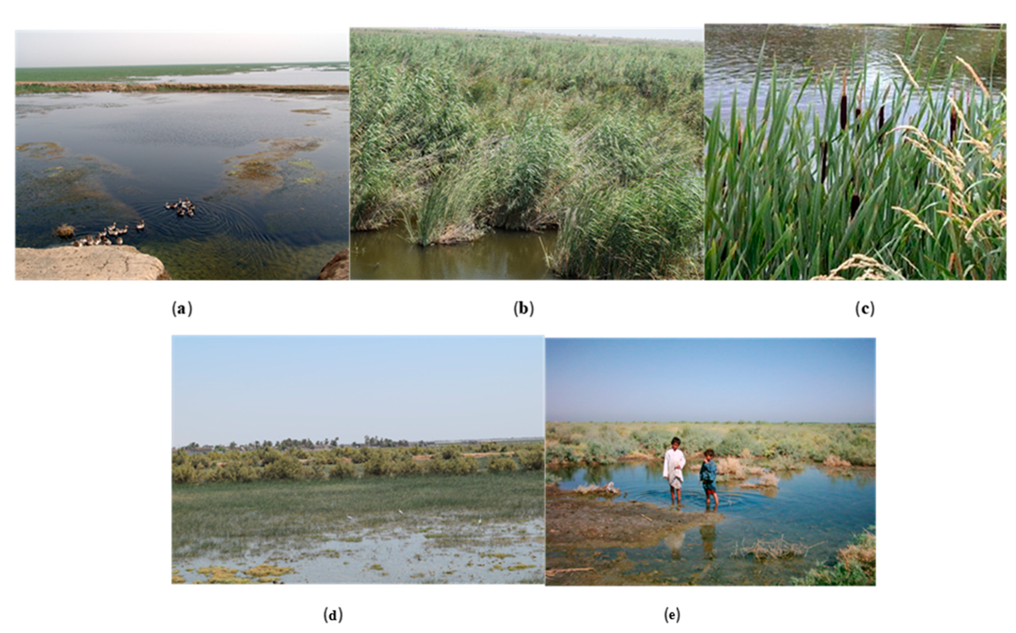
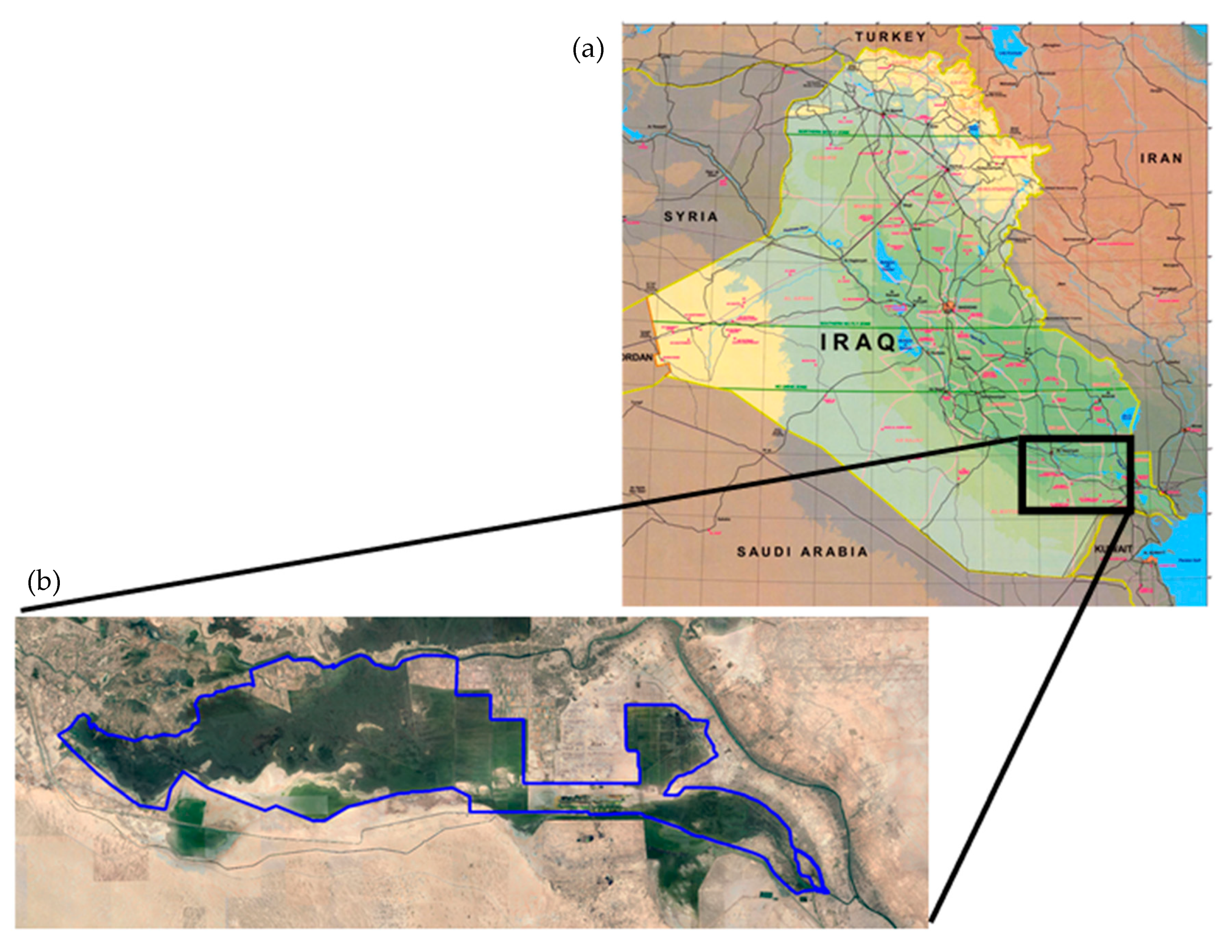
2.1. Study Area

The Iraqi Marshlands form the largest wetland system in Southwest Asia, covering more than 20,000 km2 around the confluence of the Tigris and Euphrates Rivers in southern Iraq and southwestern Iran.
In the past, the marshes served as a flood retention basin. The Al Hammar marsh is a sub-system of the Iraqi Marshlands, with an area reaching 4500 km2. Between 1991 and 1997, six canals with a total length of 5000 km were built to drain the marshes for political reasons; by 1999, the marshes became nearly dry [24,25]. Munro and Touron [11] also observed that the wetlands’ fast decline began in the early 1990s. However, nothing is known about the wetland’s health prior to the first Gulf War in the early 1980s. The UNEP estimated in 2001 that just 10% of the natural marshlands survived. By 2003, just 6% of the Al Hammar marsh was marshland [24]. The Iraqi Marshes Restoration Center (CRIM) began re-flooding it in 2004. Due to the expansion of farmlands, urban areas, and oil exploitation, the viable restoration area is now about 1600–1700 km2 [26,27,28]. It is one of the three Mesopotamian marshlands, which have been designated as Ramsar Sites under international conservation management [29]. The marsh lies south of the reach of the Euphrates River before joining the Tigris River at Al Qurna City. This reach of the river runs from Al Nasiriyah City in Al Nasiriyah Governorate to Al Chibaeich City, in the northern part of the Al Basrah Governorate. The marsh is located between latitudes 46° and 47° and longitude 30° and 30.5° and is bounded by the Euphrates River as the northern boundary, the Shatt Al Arab River as the eastern boundary, the main supply channel of the Al Basrah Water Supply Project and the Main Outfall Drain (MOD) as the southern boundary, and Suq AshShuyukh City as the western boundary (Figure 1).
The Al Hammar marsh lies within a region of high evapotranspiration. Daily data from the Al Chibaeich Meterological station located at E: 47.07, N: 30.94 (maximum and minimum temperature and relative humidity, maximum and average wind speed and the sum of solar radiation, rainfall) between 2015 and 2018 and ETo calculator software from FAO (Food and Agriculture Organisation of the United Nations) version 3.2 were used to obtain average monthly reference evapotranspiration (ETo) rates [30]; the results are shown in Figure 2. ETo reaches 300 mm per month during the summer, and a rapid approach is required for classification and monitoring in order to achieve optimum integrated water management.
One of the largest drivers which affects water cover and vegetation cover, i.e., the water balance of marshes in arid and semi-arid areas, is evapotranspiration. It is very intensive under these conditions due to high air temperatures and low atmospheric moisture content. Figure 2 shows the temperature and the reference evapotranspiration for the years 2015 to 2018. High ETo concentrated in May until October due to high temperatures, but the flow into marshland in these months is due to agriculture activities upstream. Thus, a rapid approach is required for classification and monitoring to obtain optimum water management in this area.
According to the Ramsar wetland classification system [31], the territory of the Al Hammar marsh is mainly covered with seasonal saline or brackish marshes and pools (code: Ss) and permanent saline or brackish marshes and pools (code: Sp) [29]. The local name for these seasonal brackish marshes or pools is ‘Ahwar’. There are some permanent rivers (code: M) in the area. Additionally, there are seasonal saline or brackish lakes and flats (Code: R) and permanent saline or brackish lakes (code: R). Artificial wetlands are also common in the marsh, e.g., irrigated lands (code: 3), canals, drainage channels, and ditches (code: 9).
Al-Hilli [32] described three major groups of plants in the Al Hammar: xerophyte, halophyte, and hydrophyte communities. Each of these habitats is associated with defined topographic, edaphic, and climatic conditions. Xerophytic plant communities cover the elevated semi-desert plateau around the marshes, where the soil is mostly non-saline to slightly saline. Halophytic plant communities are restricted to the lowlands with shallow water tables around areas subject to flooding. Hydrophyte communities consist of permanently submerged, partly submerged, and floating leaf plants [32].
The Al Hammar marsh comprises a system of deep and shallow lakes depending on the hydrological regime and water availability [33]. It is covered by the southern cattail (Typha domigensis), club-rush (Schoenoplectus litoralis) in the permanent marsh, and common reed (Phragmites australis) in the peripheral marsh [34,35]. In shallow lakes, pondweed vegetation is typical, such as shining pondweed (Potamogeton lucens). According to Hussain and Alwan [36], the emergent plant cover is dominated by Schoenoplectus litoralis (49.46%), Typha domingensis (36%), and Phragmites australis (22.5%), while rigid hornwort (Ceratophyllum demersum), spiny naiad (Najas marina), and sago pondweed (Potamogeton pectinatus) constituted the highest cover for submerged hydrophytes. The vegetation zonation in the Al Hammar marsh is determined by the water regime, salinity, and physical and chemical properties of the water [32].
The study reported in [36] on plant biomass of the Al Hammar marsh is particularly relevant for the present study, providing good reference data for vegetation analysis with remote sensing. The emerged plant biomass in Phragmites australis-dominated communities in the East Al Hammar marsh was 1238 g m−2 dry weight during summer. The Typha domigensis-dominated communities attained an even more moderate biomass of 111 g m−2. The Schoenoplectus litoralis communities had a biomass reaching 91 g m−2. The submerged hydrophyte biomass was dominated by Ceratophyllum demersum, at 236 g m−2. These significant differences in biomass are not surprising, as Phragmites australis forms dense communities that can reach a height of 4–6 m during the summer [37].

2.2. Analysis Methods

Characterisation of wetlands is typically achieved by analyzing the key land cover units’ spectral characteristics based on their visible and infrared reflectance. The separation of open water, vegetation, and soils is best achieved using the red (0.60–0.69 μm) and near-infrared (0.70–1.30 μm) wavelength ranges. Water shows relatively low or no reflectance in near-infrared and maximum reflectance in the blue wavelength range. Chlorophyll in healthy vegetation is a good absorber of electromagnetic energy in the visible range, especially in red, and strongly reflects in the near infrared. The different vegetation types show well detectable differences in these characteristics. Bare soil has a gradually increasing reflectance from the visible range through the near infrared to the middle infrared, depending on soil characteristics (texture, moisture content, and organic content). Historically, a combination of analog panchromatic and infrared photography has been used for such analysis, although now digital multiband scanners have become the preferred medium. A wide range of aerial and space-borne satellite imaging systems provide data over this spectral range but differ substantially in their temporal imaging frequency (overpasses per year), swath diameter, spatial resolution, and cost. The selection of imaging systems is enforced by a trade-off between these variables and must be attuned to the study’s objectives and not vice versa.
In 2010, UNEP, UNDP, and CRIM suggested a method based on NDVI to classify marshlands, and thresholds have been developed to describe the status of marsh vegetation. The UNEP study [38] showed that NDVI values greater than 0.125 represented vegetation cover. Sparse vegetation was found to correspond to NDVI values between 0.125 and 0.25, while medium-density vegetation was associated with NDVI values between 0.25 and 0.5. Dense vegetation was found to occur in areas with NDVI values above 0.5. Unfortunately, areas with NDVI values between 0.125 and 0.25 (sparse marshland vegetation) showed large commission errors, artificially expanding marshland areas. The errors resulted largely from the inability of the NDVI to differentiate between submerged sparse water vegetation and sparse terrestrial vegetation. As such, there was a need to initially delineate the marshland areas as a function of their wetness before classifying the vegetative cover status in Figure 3. Thresholding of NDMI was used for the delineation of areas with high levels of soil moisture [39]. NDMI values greater than zero were identified as wet regions [40]. Regions covered with open water were identified by their NDWI values: regions with an NDWI value greater than zero were defined as open water [41,42,43].
Three spectral indices were generated from the Landsat images to assess the temporal variability of the land cover in the marshes and the health of the vegetation cover (Table 1).
Variations in the spatial extent of the marshlands over time was assessed by the method presented in Figure 4. In the first step, open water regions were identified as the pixels with NDWI values greater than zero. Non-water cells were then separated into dry areas and wet soils or vegetated areas: if NDMI > 0, then the area is considered a vegetated area or wet but non-vegetated area. Then we used the category and thresholds defined by UNEP [38] (see above) to identify the habitat types and the dominant plants, and the land cover categories were compared with the in situ data of [32,38,44] (Table 2). The method was implemented as a model in Arc GIS 9.2. The raster layer was converted to the vector layer to calculate each class area; the areas are shown in Table A2 (Appendix A).

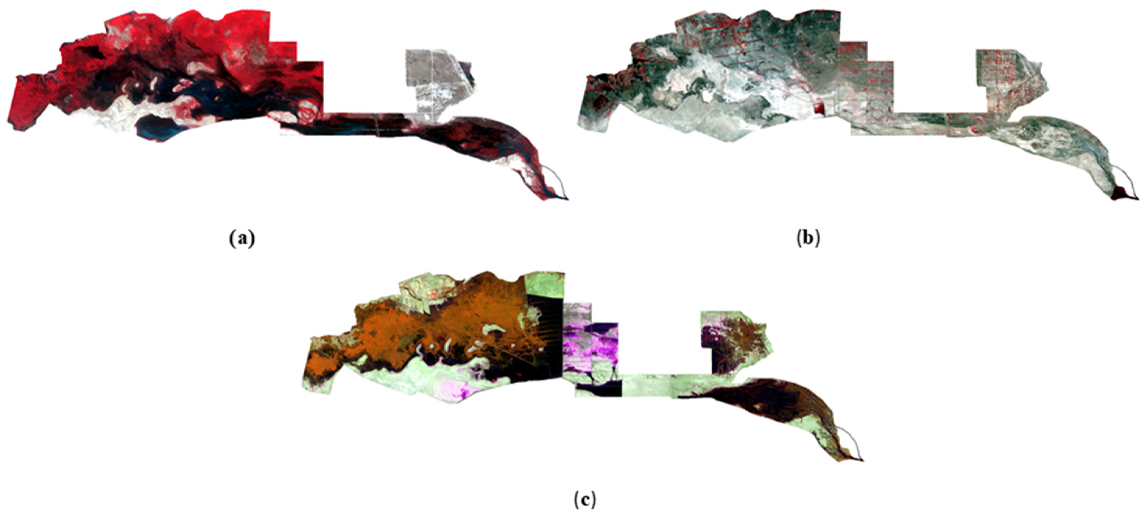
2.3. Data Download and Pre-Processing

Images from three Landsat sensors (TM, ETM, and OLI; Table A1), were used to create the time series of landcover maps of the Al Hammar marsh.
One scene was selected (path166/row 039) for each month, with cloud cover less than 10% for six years: 1991 (before degradation), 2002 (after degradation), and 2015; 2016, 2017, and 2018 for the analysis. A full breakdown of the data acquired is presented in Appendix A, Table A1. A total of 58 Landsat images were collected for the Al Hammar marsh. The available Landsat dataset for the Al Hammar marsh is non-uniform over the analysis period (some months were not represented due to cloud cover); there is a more complete record after 2013, when the data from Landsat 8 became available.

3. Results and Discussion

Rectified and enhanced false-colour composites of the marshes in July 1991, 2002, and 2017 are shown in Figure 5. Based on the methodology, the spatial extent of the marshlands was assessed in each satellite image. A visual inspection reveals the extraordinary degree of spatial changes in its extent as well as vegetative cover over the years during the study period. After a strong presence of vegetation in 1991, the 2002 image shows a near-complete lack of vegetation in the Al Hammar marsh, while there is again vegetation cover in 2017.
The spectral indices-based classification results (Figure 6, Figure 7 and Figure 8) provided the basis for the quantitative analysis shown in Figure 9. In comparison to the baseline (1991), the marsh lost a large portion of its vegetation cover up to the year 2002. This is the result of the drainage and desiccation activities carried out by the Iraqi regime during that period. The average monthly area covered with water dropped from more than 800 km2 in 1991 (Figure 6) to less than 20 km2 in 2002, as shown in Figure 7. Fortunately, recent restoration efforts have recovered some of these losses. In the past four years (2015–2018), the vegetated area has been above the 500 km2 mark 75% of the time (Figure 8 and Figure 9). However, in 2018 the vegetation and water covers are still lower than in 1991 (Figure 9). In the baseline year between April and September, vegetation and water (these two land cover classes indicate the actual extent of the wetland) covered between 1150 and 1430 km2. These land cover classes did not grow beyond 1150 km2 in 2018 (Table A2). A closer look was taken at the changes in vegetative cover over the past four years (2015–2018). The results showed the sensitivity of the marshland to droughts, the vegetation cover in 2015 (a dry year) appearing to be much lower than the levels seen in 2016, 2017, and 2018, especially in the months of August through November.
Between April and September 1991, vegetation covered between 400 and 570 km2 in the marshland. Its extent was reduced to less than 50 km2 in 2002, and 170–490 km2 in 2018. Moreover, the vegetation composition changed: the relative areas of high- and medium-density vegetation dropped in comparison to those of sparse vegetation. This shows that the recovery of the marshland has been able to reverse the dramatic degradation seen in 2002.

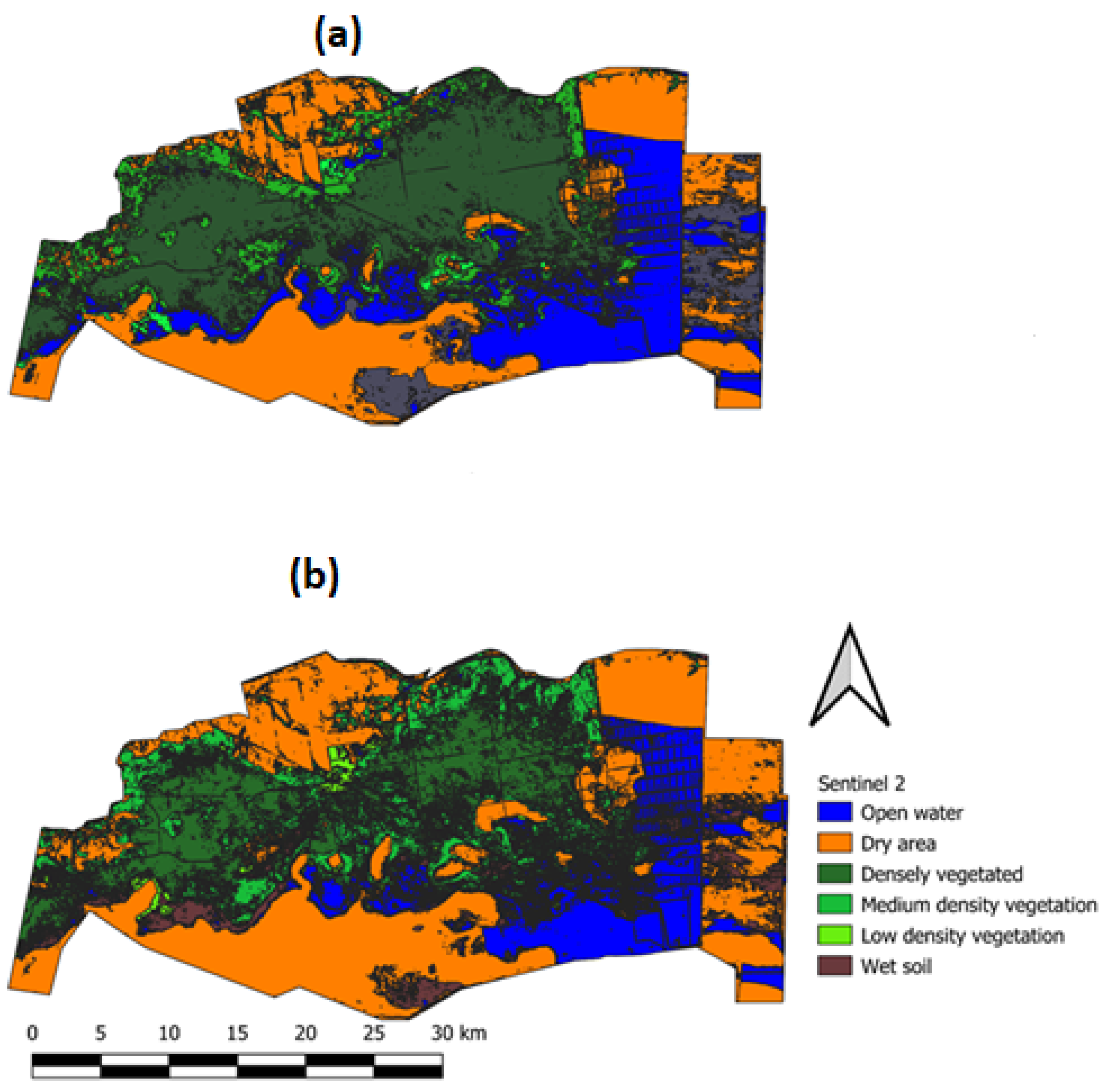
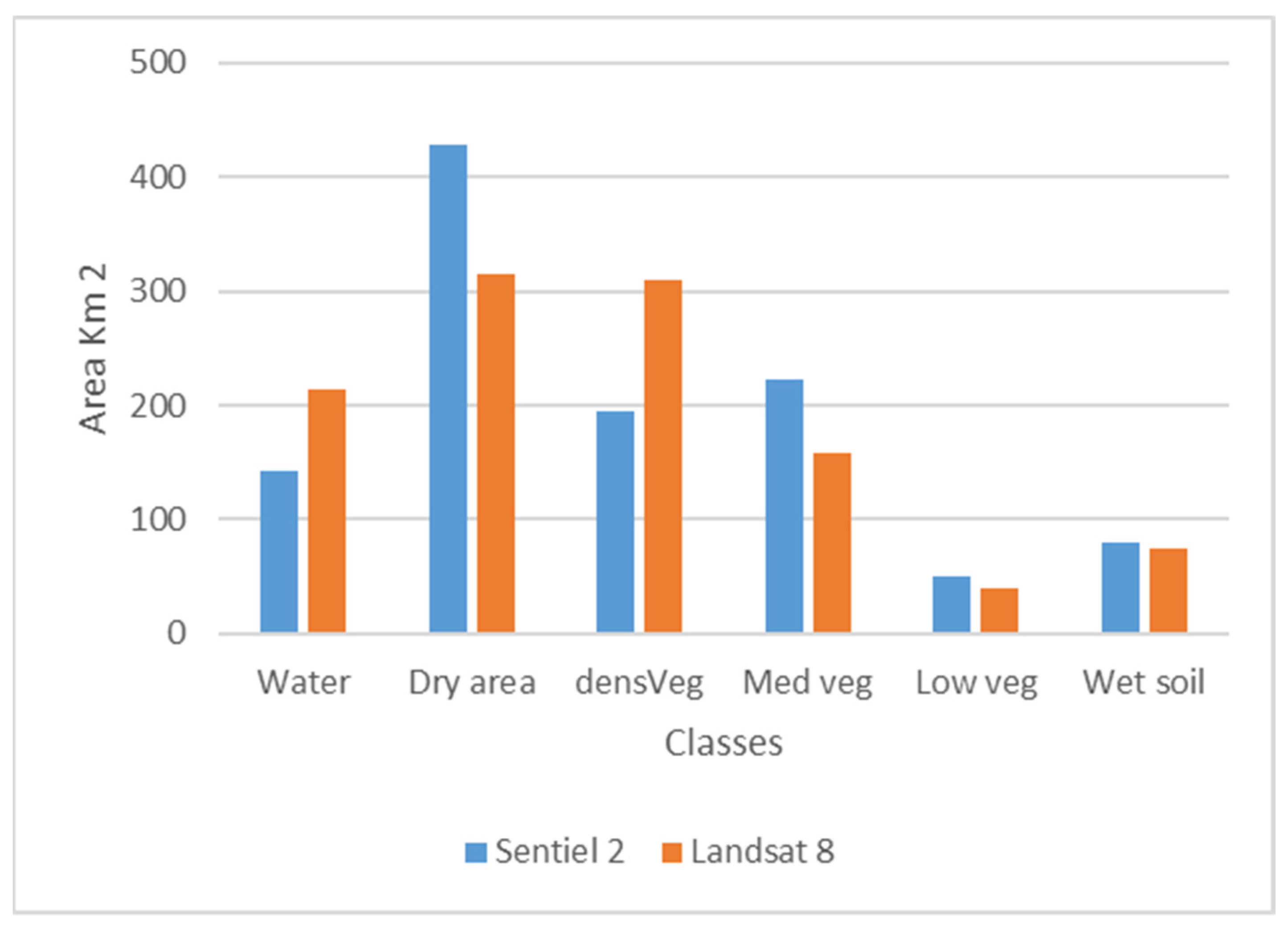
3.1. Sensitivity to Spatial Resolution

To analyse the effects of spatial resolution and using different sensors, two images from different sensors (Sentinel-2 with 10 m resolution and Landsat 8 with 30 m resolution) taken on the same day—24 August 2017—were compared. We analysed the western part of the study area, where the two images overlapped, and used the same method to classify the marshland. The results are shown in Figure 10 and Figure 11. The two resulting maps, resampled to 10 m spatial resolution, were compared in a confusion (error) matrix. The overall accuracy of the two maps was 0.78, which can be considered a good match. The complex patchy pattern of the wetland results in relatively more mixed pixels in the Landsat image, with the coarser resolution, than in the Sentinel image, leading to more mismatch of spectrally different classes (e.g., water vs. dry soil).

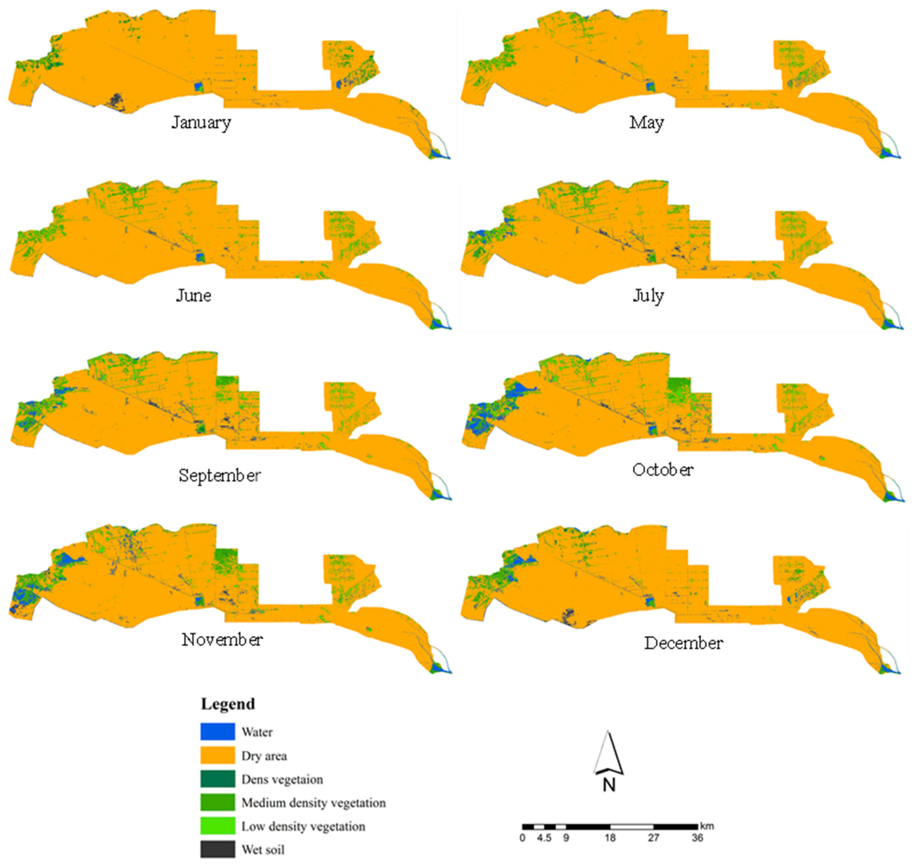
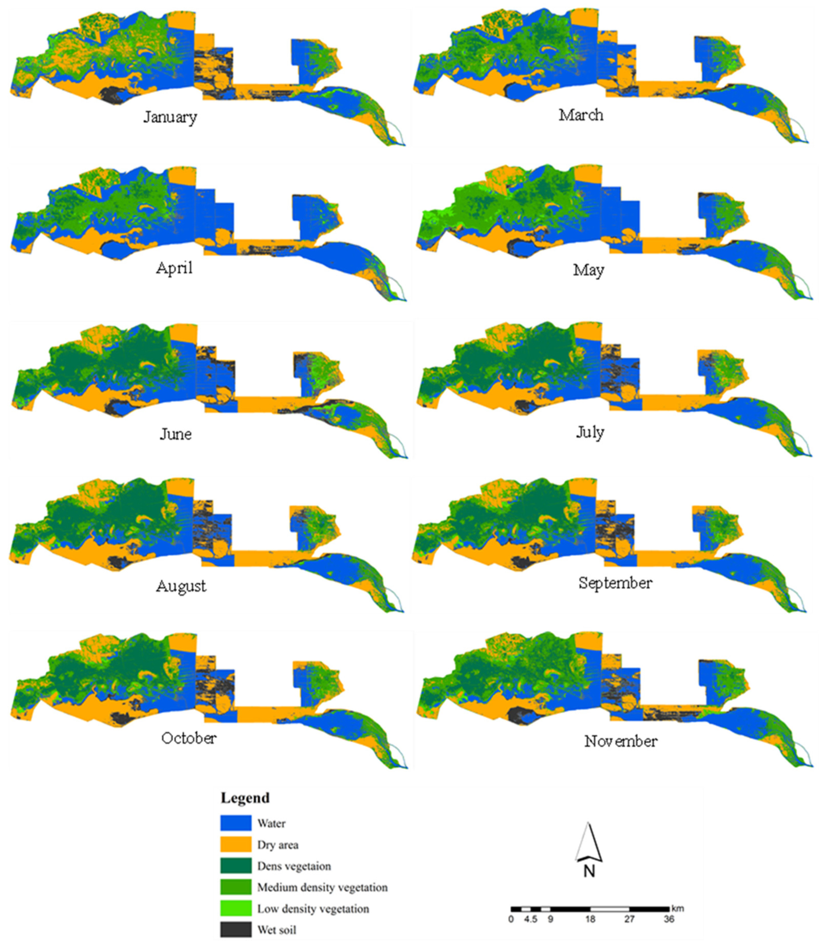
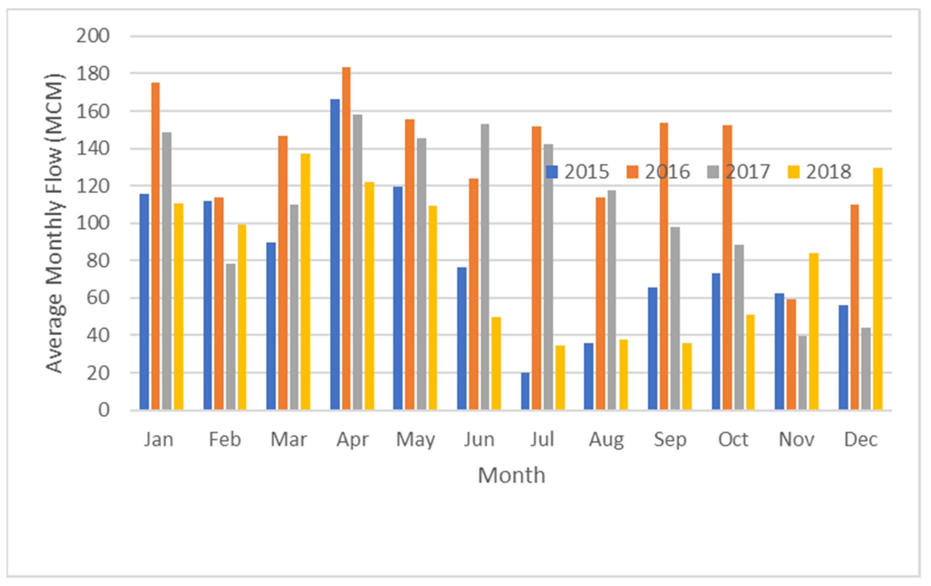
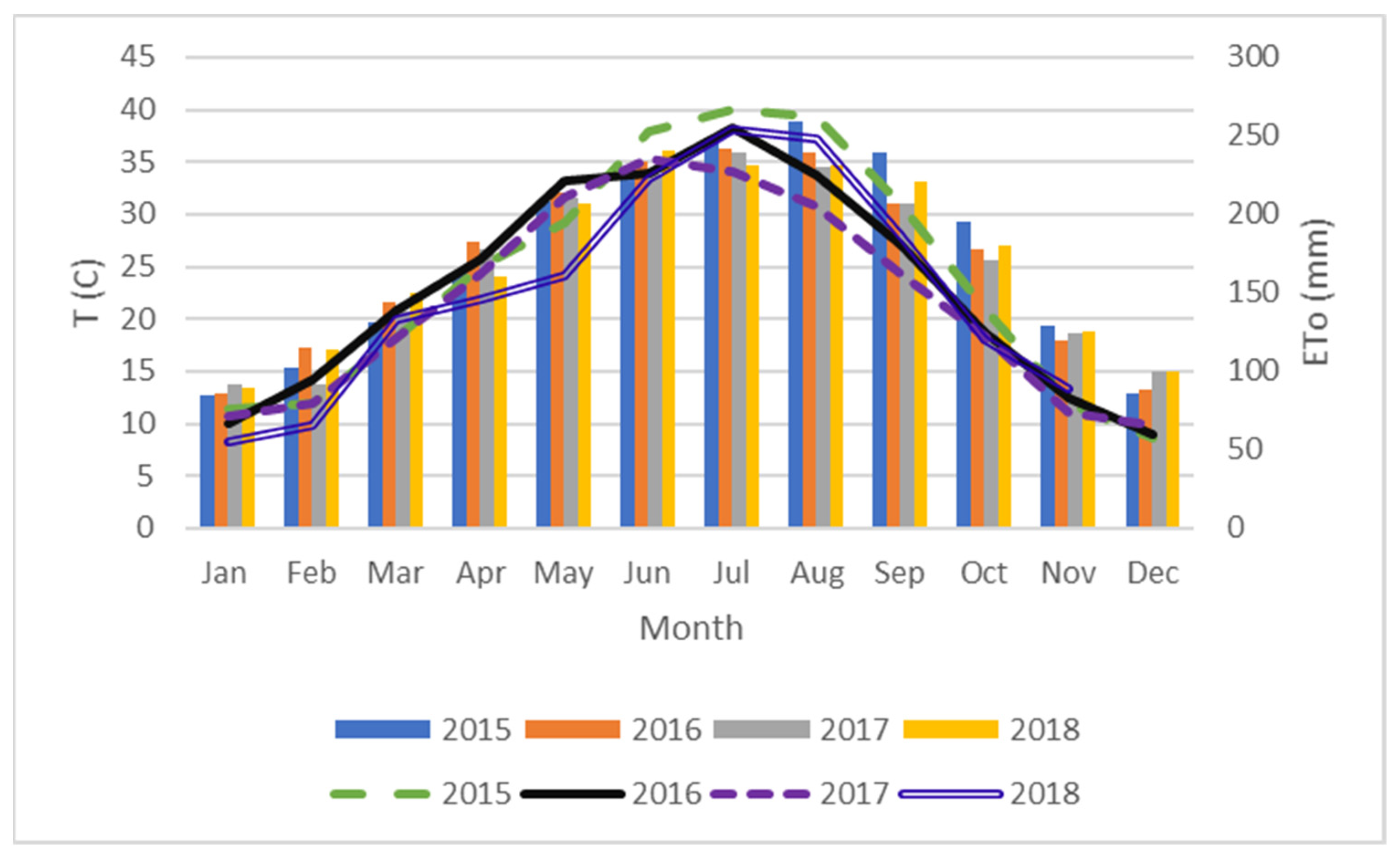
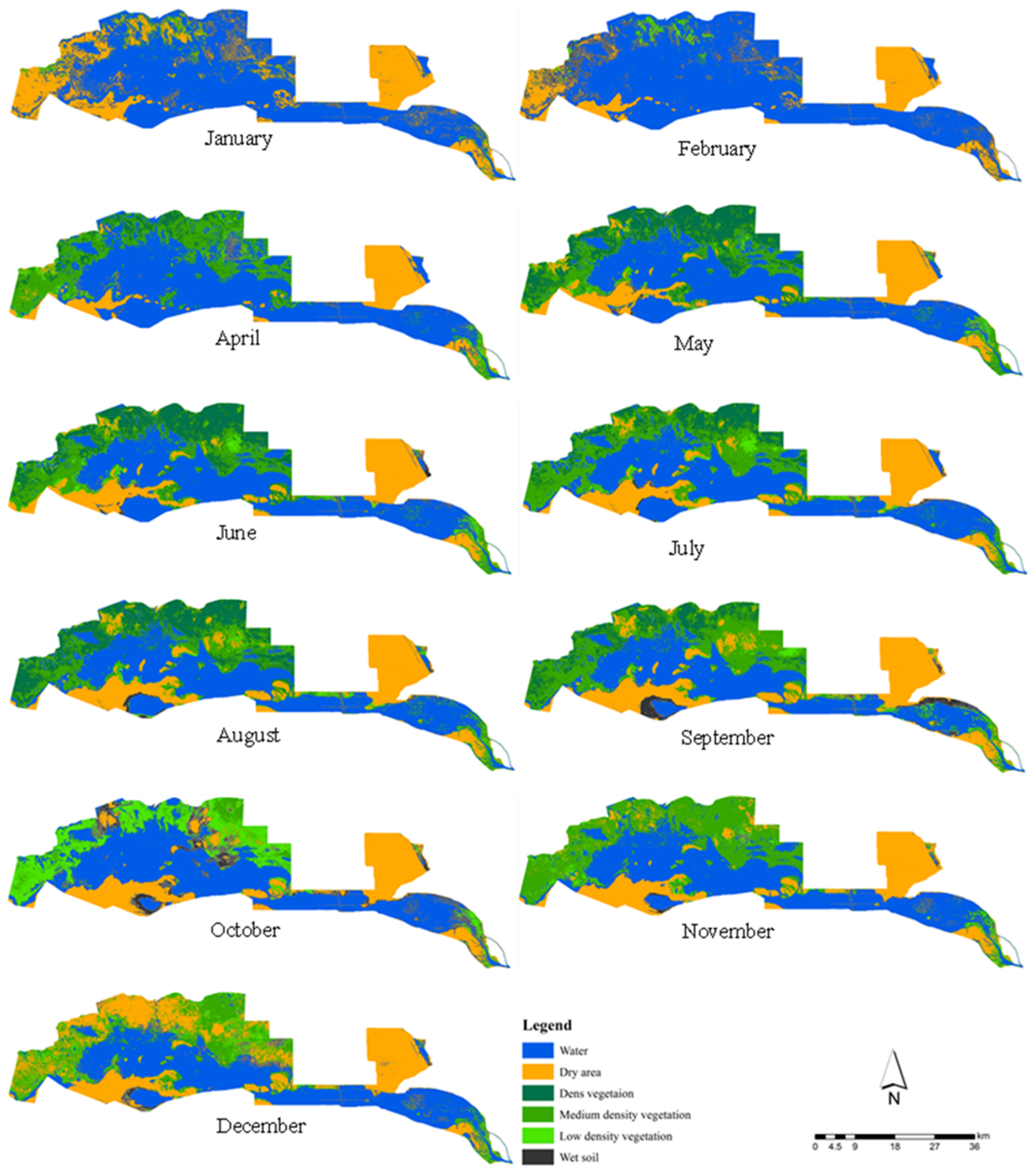
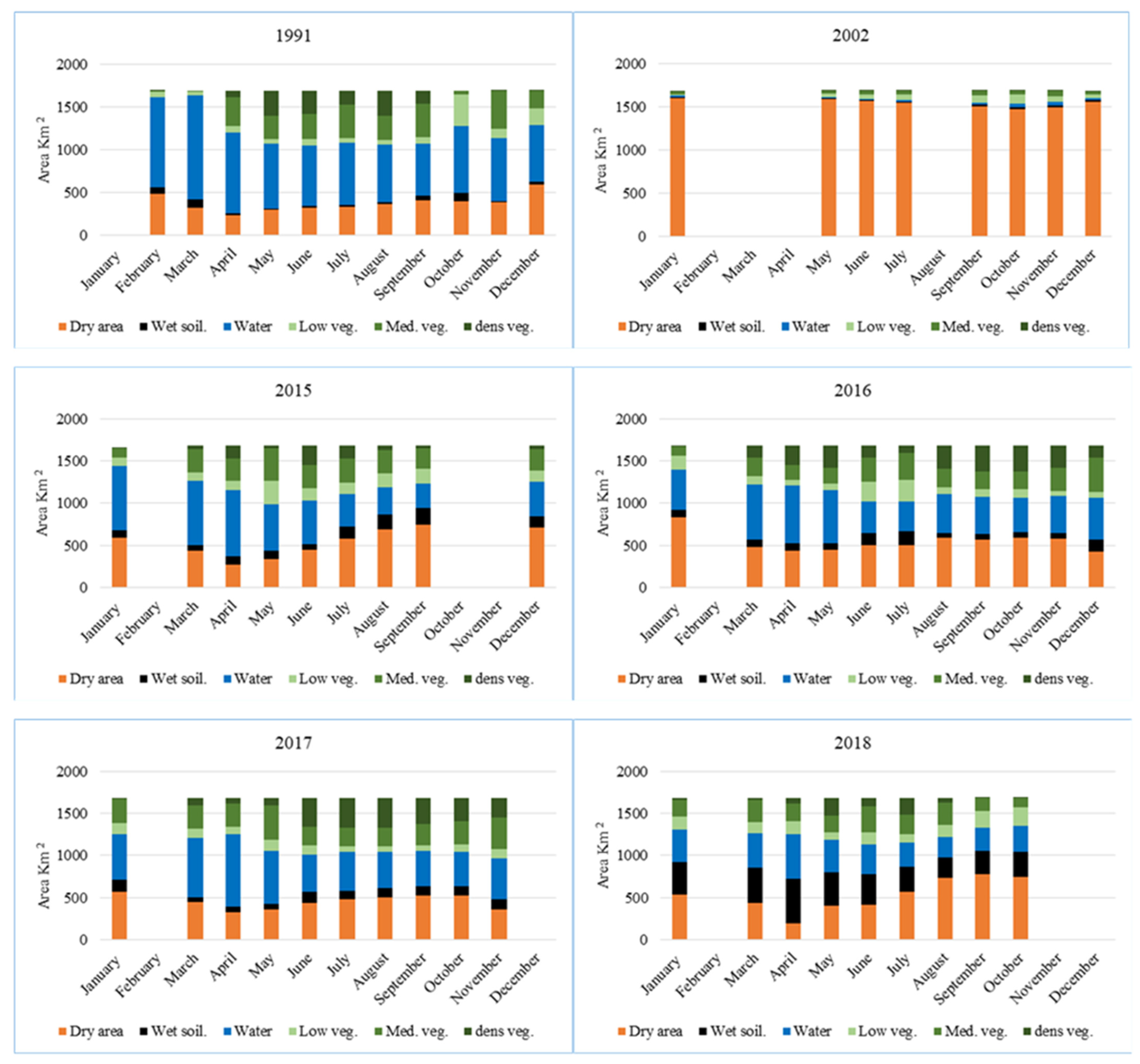
3.2. Effects of Water Availability on Land Cover

CRIW carried out monthly discharge measurements at the inlets of the main feeder canals of the marsh during the period 2015–2018 (Figure 12).
A statistical analysis was carried out to understand the relationships between the different elements of the water budget and land cover using the Statistical Package for the Social Sciences (SPSS) software. In a multivariate regression analysis, the land cover categories were tested against three predictors; the total monthly flow of the feeder canals, monthly mean air temperature, and ETo had no impact on wet soil, low vegetation, and medium vegetation. A significant positive impact of total flow on open water cover was observed, as well as negative impacts of air temperature and evapotranspiration (Table 3).

4. Conclusions

Surface reflectance image products were obtained from the USGS Earth Explorer website: http://earthexplorer.usgs.gov. accessed on 15 October 2020.
Results generated using this methodology will be critical to forecast the future state of marshlands. The revival of marshlands is based on the incoming flows affected by upstream agricultural and hydrological conditions. This approach can support the examination of existing management and restoration plans for marshlands/wetlands.
Extreme meteorological and flooding conditions in arid and semi-arid regions result in rapid and dramatic changes in the water and vegetation cover in wetlands. To understand these systems and support their management, a robust classification and monitoring method is required.
A classification approach was presented for monitoring marshlands by a hierarchical application of NDVI, NDMI, and NDWI indices calculated on the basis of optical satellite images. The proposed automatic classification results in six land cover classes, namely, (1) open water, (2) dry area, (3) dense vegetation, (4) medium-density vegetation, (5) low-density vegetation, and (6) wet soil. The proposed method uses optical indices calculated from level-2 data, allowing the use of generic thresholds.
Optical indices have been used for wetland mapping by several authors already (e.g., [45,46,47,48,49]). The approach that is proposed here uses a combination of the indices, exploiting the strength of each of them in optimally separating different land cover types. The advantage of the method is the use of fine-tuned, time-independent thresholds for a systematic and automated mapping.
For long-term monitoring, time series of Landsat images were exploited for classifying and monitoring the Al Hammar marsh (Iraq) over a time span of 29 years. To estimate the sensitivity of the method to the spatial resolution of the images, a comparison was made with the classification result of a Sentinel-2 image. Spectral differences did not affect the comparison, since the Landsat data can be combined into a systematic time series with Sentinel-2 images [45,46] Compared to the higher-resolution Sentinel-2 data, the classification showed a good overall accuracy of 0.78. Differences can be attributed to the patchy land cover pattern of the Al Hammar marsh, resulting in more mixed pixels at the 30 m resolution of the Landsat 8 images. In general, it can be concluded that the coarser resolution of the Landsat images provides sufficient accuracy for defining the land cover categories, but the much longer time series of the Landsat sensor is superior in monitoring long-term changes.
A statistical analysis was carried out to identify the direct relationships between selected variables affecting the water balance (total monthly inflow discharge, monthly air temperature, and ET) and the formation of land cover classes. A significant positive correlation between total inflow and open water cover was found. This shows that the flooding process is fast; open water cover is formed in the same month as the inflow. There was no direct effect of inflow on vegetation cover detected, since the emergence of vegetation after flooding occurs with a time delay. The reaction of vegetation cover to flooding dynamics will be a topic for further analysis.
Significant negative correlations between water cover and air temperature and evapotranspiration were also observed. This proves that these climatic factors affect water cover with high intensity due to the shallowness of the water. For maintaining stable wetland conditions, a sufficient water depth has to be achieved and maintained.
The implemented monitoring approach allowed the analysis of the flooding dynamics for a longer period, i.e., from 1991 to 2018.
The results demonstrated the changes within the marshes over the last 28 years. This analysis sheds light on the timing of major changes and allows the identification of the primary forcing variables. It was demonstrated that up until 2002 the total area covered by water and vegetation decreased to 90% of the area in 1991. As a result of the re-wetting efforts after 2002, recovery was observed, but the wetland extent did not reach the area of the baseline year of 1991.
The demonstrated method uses empirically defined and validated thresholds which might be fine-tuned with machine learning techniques. Recent research results for the classification of land cover using machine learning are promising [47,48]. Optical indices-based classification accuracies can be improved significantly [49].
Additionally, to observe the temporal and spatial patterns of land cover change using this methodology, empirical orthogonal function (EOF) analysis might be used. EOF can be used to track the temporal and spatial distributions of biomass [50,51].
The results presented here prove that this approach is suitable for classifying marshlands with land cover types of water, dry soil, wet soil, and different densities of vegetation. It can also be recommended to combine the long time series of Landsat images with new satellite data to provide more accurate classifications and increase revisiting times.
There is potential to develop our methodology to include other indices and other landcover groups. The proposed method could be adopted to efficiently classify and monitor marshlands and be used in different marshlands by changing the thresholds for NDVI, NDMI, and NDWI.

Author Contributions

Conceptualization, S.A.-M. and T.I.M.I.; methodology, S.A.-M.; software, M.M.; validation, Z.V. and G.J.; formal analysis, Z.V.; investigation, J.S.M.; data curation, S.A.-M. and T.I.M.I.; writing—original draft preparation, S.A.-M. and T.I.M.I.; writing—review and editing, Z.V. and G.J.; visualization, S.A.-M.; supervision Z.V. and G.J. All authors have read and agreed to the published version of the manuscript.

Funding

This research received no external funding.

Data Availability Statement

The datasets used in this study are available from the corresponding author on reasonable request. All data and materials are available for publication.

Acknowledgments

We acknowledge support from the Tempus Public Foundation (TPF)/Stipendium Hungaricum Scholarships Programme, Hungarian University of Agriculture and Life Sciences/Doctoral School of Environmental Sciences, Gödöllő, Hungary, and the Ministry of Water Resources, Baghdad, Iraq.

Conflicts of Interest

The authors declare no conflict of interest. The funders had no role in the design of the study; in the collection, analyses, or interpretation of data; in the writing of the manuscript, or in the decision to publish the results.

Appendix A

Table A1. Landsat data types and acquisition dates.
Date of AcquisitionSensor TypeDate of AcquisitionSensor TypeDate of AcquisitionSensor Type
22 Feberuary 1991TM12 March 2015OLI17 March 2017OLI
10 March 1991TM13 April 2015OLI02 April 2017OLI
11 April 1991TM31 May 2015OLI20 May 2017OLI
29 May 1991TM16 June 2015OLI21 June 2017OLI
14 June 1991TM18 July 2015OLI23 July 2017OLI
16 July 1991TM19 August 2015OLI08 August 2017OLI
17 August 1991TM20 September 2015OLI09 September 2017OLI
18 September 1991TM09 December 2015OLI11 October 2017OLI
20 October 1991TM10 January 2016OLI28 November 2017OLI
21 November 1991TM30 March 2016OLI15 January 2018OLI
23 December 1991TM15 April 2016OLI20 March 2018OLI
27 January 2002ETM17 May 2016OLI05 April 2018OLI
03 May 2002ETM18 June 2016OLI23 May 2018OLI
12 June 2002ETM04 July 2016OLI08 June 2018OLI
14 July 2002ETM05 August 2016OLI10 July 2018OLI
08 September 2002ETM22 September 2016OLI11 August 2018OLI
26 October 2002ETM08 October 2016OLI12 September 2018OLI
11 November 2002ETM09 November 2016OLI14 October 2018OLI
29 December 2002ETM11 December 2016OLI
23 January 2015OLI12 January 2017OLI
Table A2. Monthly land cover classification area for each class (in km2) for the years 1991, 2002, 2015, 2016, 2017, and 2018.
1991
Marsh Land CoverJanuaryFebruaryMarchAprilMayJuneJulyAugustSeptemberOctoberNovemberDecember
Dry area-486323235298322337366412394380587
Wet soil-74911815161617521061838
Water-10541225947755712724676611773742666
Low-density vegetation-6344785872615773372102195
Medium-density vegetation-7233726929438428139339442197
Densely vegetated-0069288267161287143 00
2002
Dry area1598 --159215701543-1506146914901559
Wet soil14 8615.2 19.9821.552317.7
Water14 --11915-20484125
Low-density vegetation12 --395769-89986636
Medium-density vegetation32 --344141-47466242
Densely vegetated13 --001-2125
2015
Dry area595-435268340443577688745--712
Wet soil84-67999574143184195--135
Water760-766788554520388314287--408
Low-density vegetation104-99113274143138168176--126
Medium-density vegetation112-273264388273285270244--255
Densely vegetated11-43153312311545936--48
2016
Dry area833-476433446504498595566591585428
Wet soil89-98937613916750697256141
Water474-647684631376354470441405444500
Low-density vegetation162-9970772302567686965868
Medium-density vegetation109-217172192292324213211211276407
Densely vegetated16-14723226213885279310310265140
2017
Dry area565-443331355439482504522525364-
Wet soil142-61627413597113111115119-
Water542-702865624440461427417405486-
Low-density vegetation138-1088713010465667687105-
Medium-density vegetation283-280276410221221221249272381-
Densely vegetated13-896290345356353309279228-
2018
Dry area532-436196405419573738775740--
Wet soil386-416528390355290242275308--
Water386-416528390355290242275308--
Low-density vegetation155-12715386143104138201218--
Medium-density vegetation206-267217200318224266156108--
Densely vegetated18-2363212962035911--

References

  1. Mas, J.-F. Monitoring land-cover changes: A comparison of change detection techniques. Int. J. Remote Sens. 1999, 20, 139–152. [Google Scholar] [CrossRef]
  2. Yesuph, A.Y.; Dagnew, A.B. Land use/cover spatiotemporal dynamics, driving forces and implications at the Beshillo catchment of the Blue Nile Basin, North Eastern Highlands of Ethiopia. Environ. Syst. Res. 2019, 8, 21. [Google Scholar] [CrossRef] [Green Version]
  3. Tiner, R.W.; Lang, M.W.; Klemas, V.V. Remote Sensing of Wetlands: Applications and Advances; CRC Press: Boca Raton, FL, USA, 2015; ISBN 1482237385. [Google Scholar]
  4. Guo, M.; Li, J.; Sheng, C.; Xu, J.; Wu, L. A review of wetland remote sensing. Sensors 2017, 17, 777. [Google Scholar] [CrossRef] [Green Version]
  5. Shelestov, A.; Lavreniuk, M.; Kussul, N.; Novikov, A.; Skakun, S. Exploring google earth engine platform for big data processing: Classification of multi-temporal satellite imagery for crop mapping. Front. Earth Sci. 2017, 5, 17. [Google Scholar] [CrossRef] [Green Version]
  6. Singh, A. Digital change detection techniques using remotely-sensed data. Int. J. Remote Sens. 1989, 10, 989–1003. [Google Scholar] [CrossRef] [Green Version]
  7. Dunkle, F.; Hanmer, R.; Page, R.W.; Scaling, W. Federal Manual for Identifying and Delineating Jurisdictional Wetlands; Interagency Cooperative Publication, National Service Center for Environmental Publications (NSCEP): Cincinnati, OH, USA, 1989. [Google Scholar]
  8. Tucker, C.J. Red and photographic infrared linear combinations for monitoring vegetation. Remote Sens. Environ. 1979, 8, 127–150. [Google Scholar] [CrossRef] [Green Version]
  9. Singh, A.; Harrison, A. Standardized principal components. Int. J. Remote Sens. 1985, 6, 883–896. [Google Scholar] [CrossRef]
  10. Lu, D.; Mausel, P.; Batistella, M. Land-cover binary change detection methods for use in the moist tropical region of the Amazon: A comparative study. Int. J. Remote Sens. 2005, 1, 101–114. [Google Scholar] [CrossRef]
  11. Munro, D.C.; Touron, H. The estimation of marshland degradation in southern Iraq using multitemporal Landsat TM images. Int. J. Remote Sens. 1997, 18, 1597–1606. [Google Scholar] [CrossRef]
  12. Lee, Z. Remote sensing of inherent optical properties: Fundamentals, tests of algorithms, and applications. Int. Dairy J. 2006, 1, 67–75. [Google Scholar] [CrossRef]
  13. O’Reilly, J.E.; Maritorena, S.; Siegel, D.A.; O’Brien, M.C.; Toole, D.; Mitchell, B.G.; Kahru, M.; Chavez, F.P.; Strutton, P.; Cota, G.F. Ocean color chlorophyll a algorithms for SeaWiFS, OC2, and OC4: Version 4. In SeaWiFS Postlaunch Calibration and Validation Analyses, Part 3; Academia: San Francisco, CA, USA, 2000; Volume 3, pp. 9–23. [Google Scholar]
  14. Rouse, J.W.; Haas, R.H.; Schell, J.A.; Deering, D.W. Monitoring vegetation systems in the great plains with ERTS-1. In Proceedings of the Third Earth Resources Technology Satellite-1 Symposium; Goddard Space Flight Centre, NASA: Washington, DC, USA, 1973; p. 309. [Google Scholar]
  15. Lillesand, T.M.; Keifer, R. Remote Sensing and Image Interpretation, 4th ed.; Wiley: Chichester, UK, 1999. [Google Scholar]
  16. Ozesmi, S.L.; Bauer, M.E. Satellite remote sensing of wetlands. Wetl. Ecol. Manag. 2002, 10, 381–402. [Google Scholar] [CrossRef]
  17. Schmitt, A.; Brisco, B. Wetland monitoring using the curvelet-based change detection method on polarimetric SAR imagery. Water 2013, 5, 1036–1051. [Google Scholar] [CrossRef]
  18. Dronova, I. Object-based image analysis in wetland research: A review. Remote Sens. 2015, 7, 6380–6413. [Google Scholar] [CrossRef] [Green Version]
  19. Gao, B.-C. NDWI—A normalized difference water index for remote sensing of vegetation liquid water from space. Remote Sens. Environ. 1996, 58, 257–266. [Google Scholar] [CrossRef]
  20. McFeeters, S.K. The use of the normalized difference water index (NDWI) in the delineation of open water features. Int. J. Remote Sens. 1996, 17, 1425–1432. [Google Scholar] [CrossRef]
  21. Di Vittorio, C.A.; Georgakakos, A.P. Land cover classification and wetland inundation mapping using MODIS. Remote Sens. Environ. 2018, 204, 1–17. [Google Scholar] [CrossRef]
  22. Liu, J.; Feng, Q.; Gong, J.; Zhou, J.; Li, Y. Land-cover classification of the Yellow River Delta wetland based on multiple end-member spectral mixture analysis and a Random Forest classifier. Int. J. Remote Sens. 2016, 37, 1845–1867. [Google Scholar] [CrossRef]
  23. Drexler, J.Z.; Snyder, R.L.; Spano, D.; Paw U, K.T. A review of models and micrometeorological methods used to estimate wetland evapotranspiration. Hydrol. Process. 2004, 18, 2071–2101. [Google Scholar] [CrossRef]
  24. Vinez, M.; Leonard, S. The Iraq marshlands: The loss of the garden of Eden and its people. In Proceedings of the Annual Illinois State University Conference for Students of Political Science, Chicago, IL, USA, Fall, 2010. [Google Scholar]
  25. Becker, R.H. The stalled recovery of the Iraqi marshes. Remote Sens. 2014, 6, 1260–1274. [Google Scholar] [CrossRef] [Green Version]
  26. Aoki, C.; Kugaprasatham, S. Support for Environmental Management of the Iraqi Marshlands; UNEP Publication DTI/1171/JP; United Nations Environment Programme: Nairobi, Kenya, 2009. [Google Scholar]
  27. Guarasci, B.L. Biodiversity and ecosystem management in the Iraqi Marshlands–screening study on potential world heritage nomination. J. Chem. Inf. Modeling 2011, 53, 1689–1699. [Google Scholar] [CrossRef]
  28. Center for Restoration of Iraqi Marshes. CRIMW; Annual Report; Ministry of Water Resources: Baghdad, Iraq, 2017. [Google Scholar]
  29. Ramsar Sites Information Service (RSIS) Hammar Marsh. Available online: https://rsis.ramsar.org/ris/2242 (accessed on 27 August 2021).
  30. FAO ETo Calculator. Land and Water Digital Media Series No. 36; FAO: Rome, Italy, 2009. [Google Scholar]
  31. Davis, T.J. The Ramsar Convention Manual: A Guide to the Convention on Wetlands of International Importance Especially as Waterfowl Habitat; Ramsar Convention Bureau: Gland, Switzerland, 1994. [Google Scholar]
  32. Al-Hilli, M.R. Studies on the Plant Ecology of the Ahwar Region in Southern Iraq. Ph.D. Thesis, University of Cairo, Giza, Egypt, 1977. [Google Scholar]
  33. Salim, Š.M. Marsh dwellers of the Euphrates delta. Monogr. Soc. Anthropol. 1962, 23, 157. [Google Scholar]
  34. Aqrawi, A.A.M.; Evans, G. Sedimentation in the lakes and marshes (Ahwar) of the Tigris-Euphrates Delta, southern Mesopotamia. Sedimentology 1994, 41, 755–776. [Google Scholar] [CrossRef]
  35. Evans, M.I. The Iraqi marshlands: A human and environmental study: The ecosystem; Amar International Charitable Foundation: London, UK, 2002; pp. 201–219. [Google Scholar]
  36. Hussain, D.A.; Alwan, A.A. Evaluation of Aquatic macrophytes vegetation after restoration in East Hammar marsh, Iraq. Marsh Bull. 2008, 3, 32–44. [Google Scholar]
  37. Al-Hilli, M.R.A.; Warner, B.G.; Asada, T.; Douabul, A. An assessment of vegetation and environmental controls in the 1970s of the Mesopotamian wetlands of southern Iraq. Wetl. Ecol. Manag. 2009, 17, 207–223. [Google Scholar] [CrossRef]
  38. UNDP. UNDP Technical Report. In Iraqi Marshlands Observation System; United Nations Environment Programme: Nairobi, Kenya, 2010. [Google Scholar]
  39. Hunt, E.R.; Rock, B.N. Detection of changes in leaf water content using Near- and Middle-Infrared reflectances. Remote Sens. Environ. 1989, 30, 43–54. [Google Scholar] [CrossRef]
  40. Rokni, K.; Ahmad, A.; Selamat, A.; Hazini, S. Water feature extraction and change detection using multitemporal landsat imagery. Remote Sens. 2014, 6, 4173–4189. [Google Scholar] [CrossRef] [Green Version]
  41. Fisher, A.; Flood, N.; Danaher, T. Comparing Landsat water index methods for automated water classification in eastern Australia. Remote Sens. Environ. 2016, 175, 167–182. [Google Scholar] [CrossRef]
  42. Ji, L.; Zhang, L.; Wylie, B. Analysis of dynamic thresholds for the normalized difference water index. Photogramm. Eng. Remote Sens. 2009, 75, 1307–1317. [Google Scholar] [CrossRef]
  43. Xu, C.Y.; Gong, L.; Jiang, T.; Chen, D.; Singh, V.P. Analysis of spatial distribution and temporal trend of reference evapotranspiration and pan evaporation in Changjiang (Yangtze River) catchment. J. Hydrol. 2006, 327, 81–93. [Google Scholar] [CrossRef]
  44. Salim, M.; Abd, I.; Abdulhassan, N.; Minjal, M. Key Biodiversity Survey of Southern Iraq; Nature Iraq: Sulaimani, Iraq, 2009. [Google Scholar]
  45. Kääb, A.; Winsvold, S.H.; Altena, B.; Nuth, C.; Nagler, T.; Wuite, J. Glacier remote sensing using sentinel-2. part I: Radiometric and geometric performance, and application to ice velocity. Remote Sens. 2016, 8, 598. [Google Scholar] [CrossRef] [Green Version]
  46. Mandanici, E.; Bitelli, G. Preliminary comparison of sentinel-2 and landsat 8 imagery for a combined use. Remote Sens. 2016, 8, 1014. [Google Scholar] [CrossRef] [Green Version]
  47. Varga, O.G.; Kovács, Z.; Bekő, L.; Burai, P.; Szabó, Z.C.; Holb, I.; Ninsawat, S.; Szabó, S. Validation of visually interpreted corine land cover classes with spectral values of satellite images and machine learning. Remote Sens. 2021, 13, 857. [Google Scholar] [CrossRef]
  48. Al Shehhi, M.R.; Kaya, A. Time series and neural network to forecast water quality parameters using satellite data. Cont. Shelf Res. 2021, 231, 104612. [Google Scholar] [CrossRef]
  49. Jiang, W.; He, G.; Long, T.; Ni, Y.; Liu, H.; Peng, Y.; Lv, K.; Wang, G. Multilayer perceptron neural network for surface water extraction in landsat 8 OLI satellite images. Remote Sens. 2018, 10, 755. [Google Scholar] [CrossRef] [Green Version]
  50. Liew, S.C. Spatio—Temporal Analysis of Biomass Burning In Insular Southeast Asia Using Empirical Orthogonal Function (EOF); Soo Chin Liew Centre for Remote Imaging, Sensing and Processing, National University of Singapore. In Proceedings of the 2016 IEEE International Geoscience and Remote Sensing Symposium (IGARSS), Beijing, China, 10–15 July 2016; pp. 5177–5180. [Google Scholar]
  51. Dwyer, E.; Pereira, J.M.C.; Grégoire, J.M.; Dacamara, C.C. Characterization of the spatio-temporal patterns of global fire activity using satellite imagery for the period April 1992 to March 1993. J. Biogeogr. 2000, 27, 57–69. [Google Scholar] [CrossRef]
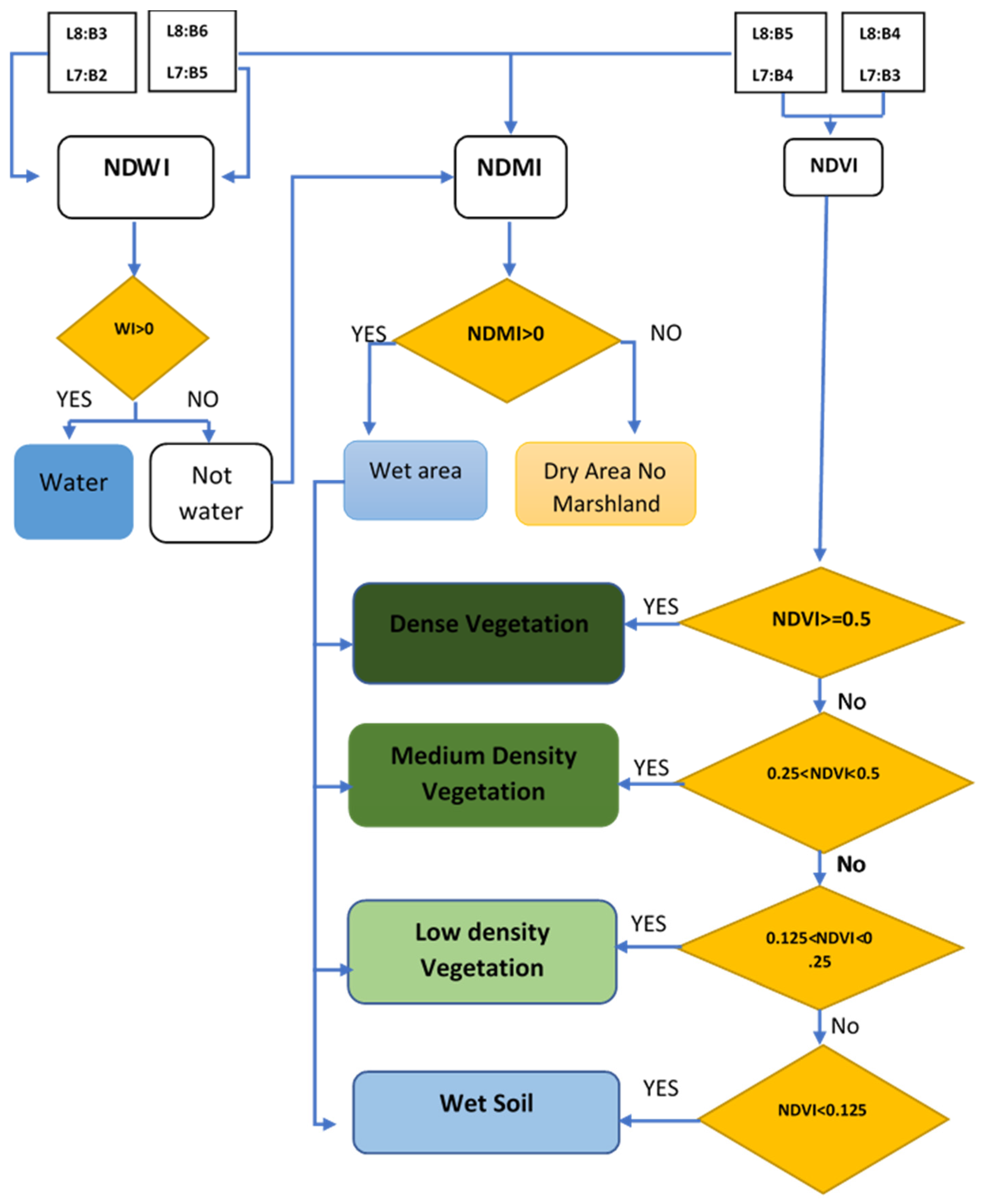
Figure 1. (a) Map of Iraq. (b) Satellite image showing the geographic location of the Al Hammar marsh with the boundary set by CRIM [28].
Water 14 01523 g001
Figure 2. Average monthly reference evapotranspiration (ETo) in the study area (represented by bars) compared with the average monthly temperature (represented by lines and dash lines) between 2015 and 2018.
Water 14 01523 g002
Figure 3. Photographs of land cover for the study area of typical habitats of the Al Hammar marsh (a) Water with pondweeds. (b) Phragmites australis community. (c) Typha domigensis community. (d) Schoenoplectus litoralis community. (e) Vegetation of wet soils. (Photos by Al-Maliki).
Water 14 01523 g003
Figure 4. Method for identifying marshland extents, open waters, and vegetated areas.
Water 14 01523 g004
Figure 5. Rectified and enhanced false-colour composites of the marshland in July of (a) 1991, (b) 2002, and (c) 2017.
Water 14 01523 g005
Figure 6. The extent of the marshland before the drains (1991).
Water 14 01523 g006
Figure 7. The extent of the marshland after the drains (2002).
Water 14 01523 g007
Figure 8. The extent of the marshland after the restoration (2017).
Water 14 01523 g008
Figure 9. Monthly changes in vegetation type and water cover areas in the Al Hammar marshland: comparison between 1991, 2002, 2015, 2016, 2017, and 2018.
Water 14 01523 g009
Figure 10. A comparison between the classification results of two different satellite images: Landsat 8 (a) and Sentinel-2 (b), for the same day.
Water 14 01523 g010
Figure 11. Histograms of the two classification results for Figure 10.
Water 14 01523 g011
Figure 12. Average monthly flow (in MCM) to the marshland between 2015 and 2018; no trend is evident, and the flow depends on the marshland’s upstream water control.
Water 14 01523 g012
Table 1. Spectral indices used to assess the Iraqi marshlands.
IndexEquation
NDVI NDVI = ( NIR R ) ( NIR + R ) [8]
NDMI NDMI = ( NIR SWIR 1 ) ( NIR + SWIR 1 ) [19]
NDWI NDWI = ( Green SWIR 1 ) ( Green + SWIR 1 ) [20]
NIR: Near infrared (Band 4 in Landsat 5 and 7; Band 5 in Landsat 8); R: Red (Band 3 in Landsat 5 and 7; Band 4 in Landsat 8); B: Blue (Band 1 in Landsat 5 and 7; Band 2 in Landsat 8); SWIR1: Shortwave infrared (Band 5 in Landsat 5 and 7; Band 6 in Landsat 8); Green: (Band 2 in Landsat 5 and 7; Band 3 in Landsat 8).
Table 2. Comparison of land cover categories based on remote sensing in this study and the habitat types of the Al Hammar marsh [32,38,44].
RS CategoriesNDVI1Habitat Type 2Dominant Plants 3
Water Rooted, submerged, helophytic and free-floating vegetation, non-vegetated river and canal (pondweed)Ceratophyllum demersum, Myriophyllum verticillatum
Dense vegetation≥0.5Flooded communities (reedbed)Phragmites australis
Medium-density vegetation>0.25, <0.5Flooded communities (reedbed)Typha domigensis
Low-density vegetation>0.125, <0.25Flooded communities (reedbed)Schoenoplectus litoralis
Wet soil Terrestrial vegetation, scrubCarex spp., Juncus spp., Tamarix spp.
Dry area Non-vegetated desertSalsola spp., Bienertia cycloptera, Hammada elegans, etc.
Table 3. Results of correlation (R) between dependent and independent variables for a statistical model.
Dry AreaWet SoilOpen WaterLow VegetationMD VegetationDense VegetationTotal Flow DischargeMonthly Air TemperatureETo (mm) Total
Dry Area1
Wet Soil0.1051
Open Water−0.675 **−0.2211
Low Vegetation0.2490.431 **−0.3161
Medium-Density Vegetation−0.510 **0.0790.0080.1271
Dense Vegetation−0.286−0.311−0.118−0.650 **−0.0831
Total Flow Discharge−0.507 **−0.2690.545 **−0.237−0.1160.2411
Monthly Air Temperature0.088−0.058−0.445 **0.214−0.0070.321 *−0.1031
ETo (mm) Total0.063−0.100−0.343 *0.236−0.0390.230−0.0290.954 **1
** Correlation is significant at the 0.01 level (two-tailed test). * Correlation is significant at the 0.05 level (two-tailed test).
Publisher’s Note: MDPI stays neutral with regard to jurisdictional claims in published maps and institutional affiliations.

