Article

Probabilistic Minimum Night Flow Estimation in Water Distribution Networks and Comparison with the Water Balance Approach: Large-Scale Application to the City Center of Patras in Western Greece

by
Athanasios V. Serafeim
1,
George Kokosalakis
1,2,
Roberto Deidda
3,
Irene Karathanasi
4 and
Andreas Langousis
1,*
1
Department of Civil Engineering, University of Patras, 26504 Patras, Greece
2
American College of Greece, Deree, School of Business and Economics Department of Maritime Transport and Logistics, 15342 Agia Paraskevi, Greece
3
Dipartimento di Ingegneria Civile, Ambientale ed Architettura Università degli Studi di Cagliari, 09123 Cagliari, Italy
4
Municipal Enterprise of Water Supply and Sewerage of the City of Patras, 26333 Patras, Greece
*
Author to whom correspondence should be addressed.
Water 2022, 14(1), 98; https://doi.org/10.3390/w14010098
Submission received: 25 November 2021 / Revised: 23 December 2021 / Accepted: 27 December 2021 / Published: 4 January 2022
(This article belongs to the Section Urban Water Management)

Abstract

:
Quantification of water losses (WL) in water distribution networks (WDNs) is a crucial task towards the development of proper strategies to reduce them. Currently, WL estimation methods rely on semi-empirical assumptions and different implementation strategies that increase the uncertainty of the obtained estimates. In this work, we compare the effectiveness and robustness of two widely applied WL estimation approaches found in the international literature: (a) the water balance, or top-down, approach introduced by the International Water Association (IWA), and (b) the bottom-up or minimum night flow (MNF) approach, based on a recently proposed probabilistic MNF estimation method. In doing so, we use users’ consumption and flow-pressure data from the 4 largest pressure management areas (PMAs) of the WDN of the city of Patras (the third largest city in Greece), which consist of more than 200 km of pipeline, cover the entire city center of Patras, and serve approximately 58,000 consumers. The obtained results show that: (a) when MNF estimation is done in a rigorous statistical setting from high resolution flow-pressure timeseries, and (b) there is sufficient understanding of the consumption types and patterns during day and night hours, the two approaches effectively converge, allowing for more reliable estimation of the individual WL components. In addition, when high resolution flow-pressure timeseries are available at the inlets of PMAs, the suggested version of the bottom-up approach with probabilistic estimation of MNF should be preferred as less sensitive, while allowing for confidence interval estimation of the individual components of water losses and development of proper strategies to reduce them.

1. Introduction

All water distribution networks (WDNs), regardless of their age and construction materials, exhibit water losses (WL). The latter are defined as the difference between the total volume of water entering a WDN in a given period of time (system input volume, SIV), and the authorized consumption (AC), and are divided into apparent and real losses. Apparent losses (AL) occur due to unauthorized consumption (UC) by illegal connections on the main WDN, metering errors at the inlets of district metered areas (DMAs) or pressure management areas (PMAs), and incorrect estimates of billed users’ consumptions. Real losses (RL) correspond to the lost water due to leakage through the pipeline connections, pipe cracks or breaks, as well as overflows in tanks and pressure wells [1,2].
Real losses (RL) are the result of all inherent (e.g., material type and properties, pipe diameters, external pipeline protection, age of the pipeline grid), functional (e.g., corrosion rate, internal pressures, external stresses, etc.) and environmental (e.g., temperature, soil erosivity, infiltration rate) factors, which affect the network from its construction and throughout its operation [3,4,5,6]. The RL volume varies between countries and WDNs, depending mainly on the condition of the network and the maintenance and monitoring capabilities of water authorities [7]. In cases of outdated and poorly maintained WDNs, RL can reach up to 70–80% of the SIV [8,9], while in some well-maintained and monitored networks, only 7% of the SIV is lost [10]. Worldwide, the non-revenue water (NRW) volume, resulting as the sum of water losses (WL) and unbilled authorized consumption (UAC), is estimated to be on the order of 126 billion cubic meters per year, conservatively valued at USD 39 billion annually [11].
Water losses undermine WDNs’ financial viability, as the lost water (which remains unbilled) results in the reduction of the net revenue while increasing the overall operational cost of the water supply agency [4,9,12,13,14]. Moreover, extensive leakages may lead to significant water quality degradation, due to undesired inflows in the case of low pressures [15,16].
Elimination of WL, apart from being not technically possible due to their nature [2,17], is also not cost-effective due to diminishing returns (i.e., the more the investment on WL reduction, the less the additional benefits [18,19,20,21]. Therefore, water supply agencies seek to determine the economic level of WL, below which any further investment is not cost-effective [22,23,24,25].
To effectively reduce WL, water agencies should first estimate them and quantify their components (i.e., RL and AL, see [26,27]). The three most common methods for WL estimation are: the water balance or top-down approach [1], the bursts and background estimates (BABE) approach (also referred to as component analysis [28]), and the minimum night flow (MNF) or bottom-up approach [29,30,31,32].
The water balance approach, which was introduced by the International Water Association (IWA [1,2]) assumes that the difference between the SIV and the legitimate authorized consumption (i.e., the sum of the billed authorized consumption and the unbilled authorized consumption) equals WL. The component of AL is estimated as a percentage of the billed consumption, based on the consumers’ characteristics of each WDN [33,34,35], and is subtracted from the total volume of WL in order to estimate the RL. In an effort to improve the WL estimates produced by the water balance approach, AL-Washali et al. [36] extended the water budget analysis to include also waste water fluxes, under the assumption that there are no leakages at the sewer system and all AL reach the waste water treatment facility. Evidently, the AL-Washali et al. [36] approach is not applicable in regions with combined sewer networks (as is the case of the city of Patras, our study area), as a large portion of the flow measured at the inlet of the waste water treatment plant originates from rainwater and groundwater discharge.
The bursts and background estimates (BABE) approach is used to estimate the RL components (burst losses and background losses), which are quantified in a semi-empirical context [28]. In a later study, Lambert et al. [37] proposed that the largest portion of the RL volume is avoidable, and the remaining part can be assessed using the unavoidable annual real losses (UARL) factor [38], which is defined as the lowest achievable RL for a specific pressure in a well-managed WDN. The application of BABE method requires identification of all repaired bursts (reported or unreported) in the WDN, as well as the time period between their detection and eventual repair [39].
The minimum night flow (MNF) method, which is the most popular approach for RL estimation in WDNs, is commonly applied in district metered areas (DMAs, hydraulic isolated areas/zones of a WDN, see [40]) or pressure management areas (PMAs, i.e., DMAs where pressure management is applied) under the assumption that human activity during the late night and early morning hours is minimal [5,41]. Therefore, MNF estimates can be considered representative of background losses, defined as the sum of small and possibly undetectable leaks, the localization and repair of which is deemed economically unprofitable [42], unless the water loss is gradually increased to the point where it is possible to detect and repair them in a cost-effective setting [43,44].
An important issue in MNF estimation from flow timeseries, is that there are no rigorous methodological specifications for its implementation. For example, depending on the application and the networks’ monitoring characteristics, extraction of night flow minima may start (end) at different night (morning) hours, usually ignoring the resolution of the data and the seasonality of the consumption [5,31,45,46,47,48,49,50,51,52,53]. To bridge this gap, in a recent study, Serafeim et al. [42] developed two conceptually different probabilistic approaches for MNF estimation, which are based on statistical metrics, and are suited to minimize noise effects, allowing for more accurate representation of the low flows during night hours, as well as confidence interval estimation of the observed MNFs, making them more suitable for practical applications.
The purpose of this work is to compare the effectiveness and robustness of WL estimation approaches found in the international literature, based on a large-scale, real-world application in selected PMAs of the WDN of the city of Patras, the third largest city in Greece. Since there are no available burst records for the WDN of the city of Patras (required for effective application of BABE method) and, also, its sewer network is combined, comparison is limited to: (a) the water balance or top-down approach introduced by IWA, and (b) the bottom-up approach based on MNF estimates obtained by applying the probabilistic approach for MNF estimation by Serafeim et al. [42].
The rest of the manuscript is organized as follows: Section 2 provides important information about the area of application and the available data. The applied methodologies are briefly outlined in Section 3, while important comparative results are presented and discussed in Section 4. Conclusions and future research directions are summarized in Section 5.

2. Data

In the analysis that follows, we use consumption (billed and unbilled) and flow-pressure data, which have been collected from the 4 largest pressure management areas (PMAs, namely Boud, Kentro, Panahaiki and Prosfygika, see Figure 1) of the city of Patras in western Greece, with continuous supply.
The selected PMAs consist of more than 200 km of pipeline (mainly HDPE and PVC pipes), cover the entire city center of Patras, and serve approximately 58,000 consumers (based on data from the Hellenic Statistical Authority and the Municipality of Patras), which correspond to more than 44,000 active hydrometers (see Table 1). The 4 PMAs have uniform characteristics regarding population and building densities, land uses (which are mostly commercial and residential) and topography, as they lie along the coastline of the gulf of Patras, with minimal altitude differences.
The 4 selected PMAs are part of the “Integrated System for Pressure Management, Remote Operation and Leakage Control of the Water Distribution Network of the City of Patras”, which is the largest smart water network (SWN) in Greece, with the Municipal Enterprise of Water Supply and Sewerage of the City of Patras (DEYAP) acting as the competent Authority for its operation and management [54,55].
Users’ consumption and flow-pressure data, for each of the 4 PMAs, were acquired by DEYAP, during the 4-month long period from 1 November 2018 to 28 February 2019 (i.e., 119 days), which corresponds to the low-consumption period of the year (i.e., in the case of Greece, this period corresponds to the months from November to February [55,56,57]). It is important to note that all 4 PMAs did not exhibit any prolonged periods of malfunctioning and/or pressure regulation issues. Data were, first, quality assessed in order to remove any errors related to data transmission system malfunctions (i.e., communication glitches of the 3G transmission system [42]).

3. Methodology

In the next two subsections, we briefly describe the water balance (or top-down) approach introduced by IWA, and the bottom-up approach based on MNF estimates obtained by applying the probabilistic approach of Serafeim et al. [42], in order to estimate the water losses (WL) in WDNs and their decomposition into real losses (RL) and apparent losses (AL). A detailed review regarding the steps of the top-down and bottom-up approaches is presented in AL-Washali et al. [40].

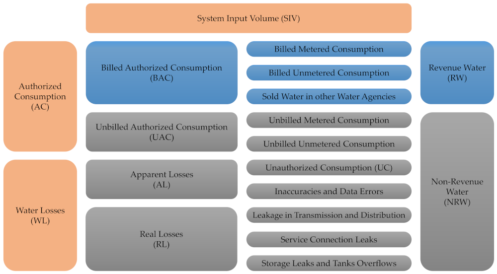
3.1. Water Balance (Top-Down) Approach

The International Water Association, through its Water Loss Task Force, established the concept and developed the necessary methodology to calculate water balances in WDNs [30], which can be applied at both WDN (system-wide [41]) and DMA scales. In order to apply the method, the total system input volume (SIV) should be determined, as well as the authorized consumption (AC), which can be billed or unbilled. It should be noted that the billed authorized consumption (BAC) is the consumption of water by legal users/consumers (also referred to as revenue water, RW), which is billed for the financial benefit of the water agency and can be metered or non-metered. The latter is calculated using mean consumption volumes, which are estimated based on the nature and specific characteristics of each consumer. Billed authorized consumption includes, also, water sold in areas outside the WDN.
The WL volume is estimated by subtracting the unbilled authorized consumption (UAC, metered or unmetered) from the non-revenue water (NRW) (see Equation (1)), with the latter being calculated by subtracting the billed authorized conception (BAC) from the system input volume (SIV) (see Equation (2)).
WL = NRW − UAC
NRW = SIV − BAC
As WL corresponds to the sum of real losses (RL) and actual losses (AL):
WL = RL + AL
In order to estimate RL from Equation (3), one needs to first quantify the AL volume through its components (i.e., unauthorized consumption (UC), systematic metering errors, and inaccurate estimates of billed users’ consumptions) using semi-empirical estimates met in the international literature [34].
For example, in high-income countries, the UC volume is commonly assumed to be on the order of 0.1% [34] or 0.25% [33] of the SIV. In low-income countries, however, the corresponding UC estimates are higher, on the order of 10% of the BAC [35] or 10% of the NRW [58]. Systematic metering errors at the inlets of PMAs and/or DMAs should be estimated using flow tests under the meters’ manufacturers’ guidance [59,60]. Inaccurate estimates of billed users’ consumptions can be identified using historical flow timeseries and the corresponding billing data.
In summary, the assessment of AL is conducted by the water agencies, based on their experience and the technical specifications of the data recording and transmission systems. Figure 2 below presents a schematic illustration of the water balance components considered in WDNs as proposed by IWA [1].

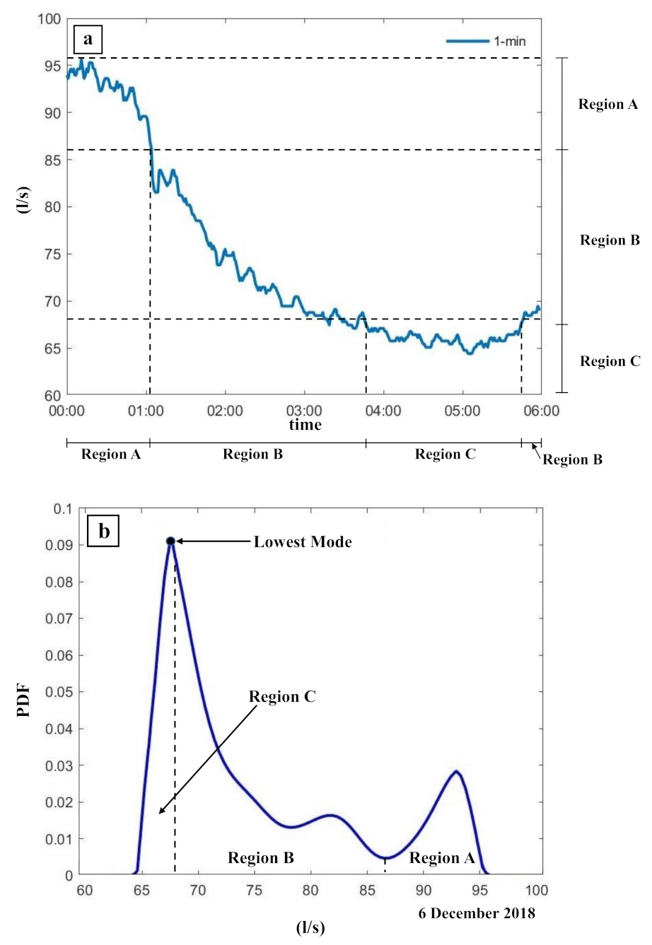
3.2. Minimum Night Flow (Bottom-Up) Approach

Based on the concept that human activity is minimal during late night and early morning hours, the minimum night flow (MNF) method uses flow data at the inlet of a DMA (or PMA) to estimate flow minima, which can be considered representative of the background losses. In cases of intermittent supply WDNs, the minimum flow can occur at any time of the day, but most likely during morning hours [41].
As noted in the Introduction, most MNF estimation approaches are based on extraction of flow minima observed during night hours and ensemble averaging of the results. In a recent study, Serafeim et al. [42] developed two probabilistic approaches for MNF estimation based on statistical metrics, which produce robust estimates based on average night flow conditions during the low-consumption period of the year. In the first approach, a proper scale for temporal averaging of night flows is identified and used to filter out noise effects in the obtained MNF estimates. The second approach is more intuitive, estimating MNF as the ensemble mean of the lowest modal values (i.e., the most probable states of night flows) observed during the night hours of each day in the low-consumption period of the year. Since the second method is simpler to apply and both Serafeim et al. [42] approaches lead to very similar results, in what follows, we use the second approach for MNF estimation.
To illustrate the adopted MNF estimation method, Figure 3a shows the 1-min resolution timeseries of flow measurements in PMA “Kentro” on 6 December 2018, within the time frame from 00:00 am to 06:00 am, and Figure 3b presents its corresponding empirical probability density function (ePDF).
One clearly sees that the empirical distribution is characterized by three distinct Regions: Region A spans from 00:00 am to 01:05 am (late night; see Figure 3a), Region B is composed by flow values observed between 01:05 am–03:50 am (late night) and 05:45 am–06:00 am (early morning), and Region C includes the low flows during the night hours from 03:50 am to 05:45 am. We observe that the lowest modal value (i.e., the lowest most frequent value) of the distribution is observed in Region C, and can be considered representative of the MNF, as the latter is linked to the most probable low-consumption state of the DMA during night hours, when human activity is minimal. For more details regarding the MNF estimation method, the reader is referred to Serafeim et al. [42].
After estimating the MNF for a selected PMA or DMA, one needs to decompose it to net night flow (NNF, which equals the leakage rate during night hours [61]), and users’ night consumption (UNC, which can be both authorized and unauthorized), through the balance equation:
NNF = MNF − UNC
UNC can be estimated based on the assumption that approximately 6% of the domestic population is active during the night hours, with consumption equal to 10 L of water per capita [62]. For non-domestic consumers, the exact night consumption is metered on site.
Since NNF corresponds to the leakage rate during night hours when pressures in the network are generally lower (due to pressure management), to obtain the real losses (RL) occurring during both night and day hours, the NNF should be multiplied by the night-day factor (NDF [63]):
RL = NNF   ×   NDF , NDF = i = 0 24 P i P M N F N 1
where RL is in m3, NNF is in m3/h, Pi is the mean pressure during each hour i of the day, PMNF denotes the mean night pressure during the period of MNF estimation, and N1 is the so called leakage exponent taking values from 0.5 for rigid (i.e., steel, cast iron, plain concrete, reinforced concrete, vitrified clay, and asbestos cement) pipes, to 1.5 for flexible (PE, PVC, HDPE, FRP, etc.) pipes [34,63,64,65], with average value on the order of 1.15 [63,64].
In the next section, we compare the results obtained by applying the water balance or top-down approach presented in Section 3.1, and the bottom-up approach based on Serafeim et al. [42] MNF estimation method presented in Section 3.2, to the 4 largest PMAs of the city of Patras in western Greece (i.e., Boud, Kentro, Panahaiki and Prosfygika; see Figure 1 and Table 1). In doing so, we utilize users’ consumption and flow-pressure data during the 4-month long low consumption period from 1 November 2018 to 28 February 2019 (i.e., 119 days; see Section 2).

4. Application and Results

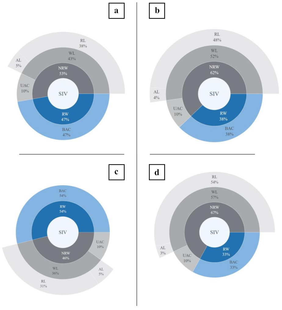
4.1. Water Balance (Top-Down) Approach

Table 2 summarizes the components of the water balance approach for the 4 PMAs of Patras WDN, obtained by applying Equations (1)–(3) to flow timeseries and users’ consumption data provided by DEYAP.
The unbilled authorized consumption (UAC) has been set to 10% of the system input volume (SIV), while apparent losses (AL) have been set to 10% of the billed authorized consumption (BAC), similar to cases of low-income countries [35,58,66]. The aforementioned percentages have emerged from additional studies conducted by DEYAP in the recent past and are considered representative of the entire city center of Patras. The AL component originates mostly from unauthorized consumption (UC) and inaccurate estimation of billed users’ consumptions, as metering errors at the inlets of the 4 selected PMAs, which belong to “Integrated System for Pressure Management, Remote Operation and Leakage Control of the Water Distribution Network of the City of Patras” (see Section 2), can be considered negligible.
To further investigate the water balance equilibrium, Figure 4 illustrates the allocation of the system input volume (SIV) into revenue water (RW, also referred to as billed authorized consumption, BAC) and non-revenue water (NRW) and their sub-components. NRW consists of the unbilled authorized consumption (UAC) and the water losses (WL) component, with the latter being equal to the sum of apparent losses (AL) and real losses (RL). One sees that with the exception of PMA 3 (Panachaiki, see Figure 4c), most of the water entering PMAs 1 (Boud, see Figure 4a), 2 (Kentro, See Figure 4b) and 4 (Prosfygika, see Figure 4d) remains unbilled (NRW, 53%, 62% and 67%, respectively), with real losses (RL) constituting its largest portion (38%, 48% and 54%, respectively), most probably due to excessive leakages and background losses.

4.2. Minimum Night Flow (Bottom-Up) Approach

Table 3 shows the mean values, standard deviations and 95%-confidence intervals of the MNF estimates for the 4 selected PMAs of Patras WDN, obtained using the Serafeim et al. [42] approach, and Table 4 presents the 95%-confidence intervals of the components of the bottom-up (or minimum night flow) approach (i.e., UNC, users’ night consumption; NNF, net night flow; NDF, night-day factor; RL, real losses) using the 95%-confidence intervals in Table 3 and Equations (4) and (5).
The domestic component of UNC has been estimated using the Hamilton and McKenzie [62] assumption (see Section 3.2), while the non-domestic one has been estimated by DEYAP to be on the order of 15% of the MNF for PMAs 1 and 4 (Boud and Prosfygika, respectively), and 30% for PMA 2 (Kentro, which corresponds to the city center with pronounced night activity; i.e., mostly dining areas, bars and night clubs). PMA 3 (Panachaiki) is entirely residential, not exhibiting any non-domestic night consumption.
The night-day factors (NDFs) in Table 4 have been obtained by applying Equation (5) for N1 = 1.15, using the hourly means of the pressure set points acquired from the 1-min resolution timeseries during the 4-month low consumption period (see Section 3.2). Table 5 summarizes the average (over the whole period of MNF estimation) pressure set points during the night (i.e., 00:00 a.m.–6:00 a.m.) and day (i.e., 06:00 a.m.–00:00 a.m.) hours, where one sees that irrespective of the PMA considered, the differences in the applied pressures between day and night hours are minimal.

4.3. Comparison between Approaches

Table 6 summarizes the RL estimates obtained using the water balance (top-down) and minimum night flow (bottom-up) approaches, expressed as fractions of the SIV. One sees that the two approaches lead to very similar results, with absolute relative differences lower than 10% for all 4 PMAs (7.28%–7.99%, 2.30%–4.39%, 1.25%–5.77% and 8.01%–9.54% for PMAs Boud, Kentro, Panachaiki and Prosfygika, respectively). The aforementioned finding indicates that: (a) when the network’s specific characteristics are known and there is sufficient understanding of the consumption types and patterns during day and night hours, and (b) MNF estimation is done in a rigorous statistical setting from high resolution flow-pressure timeseries, the top-down (water balance) and bottom-up (MNF) approaches effectively converge, allowing for more reliable estimation of the individual components of water losses and identification of proper strategies to reduce them.

5. Conclusions

Estimation of water losses (WL) is a crucial task for all water agencies, as they undermine the WDNs’ financial and environmental viability. The most common WL estimation methods are the IWA’s water balance (or top-down) approach, the bursts and background estimates (BABE, or component analysis) approach, and the minimum night flow (MNF, or bottom-up) approach. While widely applied, the aforementioned WL estimation methods are not limitation-free. For example, IWA’s top-down approach relies on semi-empirical assumptions for the estimation of both unbilled authorized consumption (UAC) and apparent losses (AL), with high levels of uncertainty that may create inaccuracies on the order of 200% [41]. On the other hand, the bottom-up approach is affected by MNF estimation uncertainties originating mostly from the quality and resolution of the available flow-pressure timeseries, the estimation method applied to extract flow minima (see Introduction), as well as the representativeness of the assumed users’ night consumption (UNC).
In an effort to improve the accuracy and robustness of the bottom-up approach, Serafeim et al. [42] developed a probabilistic framework for MNF estimation in WDNs, based on statistical metrics, that filters out noise effects, estimating MNF as the average flow of the most probable states during the night hours of the low-consumption period of the year. The strong point of the developed approach for MNF estimation, is that it is easily applicable while allowing for both point and confidence interval estimation of the average MNF and, consequently, of all components of the bottom-up approach (i.e., users’ night consumption, UNC, net night flow, NNF, and real losses, RL). The application of the water balance (or top-down) and bottom-up (with Serafeim et al. [42], probabilistic MNF estimation procedure) approaches to the 4 largest and most studied (by the competent authority, DEYAP) PMAs of the WDN of the city of Patras, showed that: (a) when MNF estimation is done in a rigorous statistical setting from high resolution flow-pressure timeseries (with regard to the bottom-up approach), and (b) there is sufficient understanding of the consumption types and patterns during day and night hours (with regard to the water balance, or top-down approach), the two approaches effectively converge, allowing for more reliable estimation of the individual components of water losses.
Under this setting, when high resolution flow-pressure timeseries are available at the inlets of PMAs, the suggested version of the bottom-up approach with probabilistic estimation of MNF should be preferred as less sensitive, not requiring semi-empirical assumptions for both the unbilled authorized consumption (UAC) and the apparent losses (AL), while allowing for confidence interval estimation of the individual components of water losses and development of proper strategies by the competent authorities in order to reduce them. In the case of intermittent water supply systems, such as those implemented in several developing regions, MNF estimation is still applicable, but in this case, the analysis should not be limited solely to night hours, but be extended so that it encompasses the entire daily water supply schedule. Future communications will focus on advancing the developed framework to allow for parameterization of WL components as a function of PMA specific characteristics (i.e., pipe diameters, length of the pipeline grid, operating pressures, etc.).

Author Contributions

Conceptualization, methodology, investigation, A.V.S. and A.L.; data curation, formal analysis, validation, visualization, writing—original draft preparation, A.V.S.; writing—review and editing, G.K., R.D., I.K. and A.L.; supervision, project administration, funding acquisition, A.L. All authors have read and agreed to the published version of the manuscript.

Funding

The research project was supported by the Hellenic Foundation for Research and Innovation (H.F.R.I.) under the “1st Call for H.F.R.I. Research Projects to support Faculty Members & Researchers and the procurement of high-cost research equipment grant” (Project Number: 1162).

Institutional Review Board Statement

Not applicable.

Informed Consent Statement

Not applicable.

Data Availability Statement

The flow-pressure data used in the present study are protected under a nondisclosure agreement. Interested parties can ask for access directly from the Municipal Enterprise of Water Supply and Sewerage of Patras (DEYAP; https://www.deyap.gr; last accessed on 2 November 2020).

Acknowledgments

The authors would like to acknowledge the useful comments and suggestions received by two anonymous reviewers, which significantly helped to improve the presentation of the developed concepts.

Conflicts of Interest

The authors declare no conflict of interest.

Abbreviations

ACAuthorized Consumption
ALApparent Losses
BABEBursts and Background Estimates
BACBilled Authorized Consumption
DEYAPMunicipal Enterprise of Water Supply and Sewerage of the City of Patras
DMADistrict Metered Area
ePDFempirical Probability Density Function
FRPFiber-Reinforced Polymer
HDPEHigh Density Polyethylene
IWAInternational Water Association
MNFMinimum Night Flow
N1Leakage exponent
NDFNight-Day Factor
NNFNet Night Flow
NRWNon-Revenue Water
PDFProbability Density Function
PEPolyethylene
PiMean pressure during each hour i of the day
PMAPressure Management Area
PMNFMean night pressure during the MNF estimation period
Ps,dPressure set point during day
Ps,nPressure set point during night
PVCPolyvinyl Chloride
RLReal Losses
RWRevenue Water
SIVSystem Input Volume
SWNSmart Water Network
UACUnbilled Authorized Consumption
UARLUnavoidable Annual Real Losses
UCUnauthorized Consumption
UNCUsers’ Night Consumption
WBWater Balance
WDN Water Distribution Network
WLWater Losses
μMNEnsemble mean of the individual MNF estimates
σMNFStandard deviation of the individual MNF estimates

References

  1. Lambert, A.; Hirner, W. Losses from Water Supply Systems: A Standard Terminology and Recommended Performance Measures; IWA Publishing: London, UK, 2000. [Google Scholar]
  2. Lambert, A.; Charalambous, B.; Fantozzi, M.; Kovac, J.; Rizzo, A.; Galea, S. 14 years experience of using IWA best practice water balance and water loss performance indicators in Europe. In Proceedings of the IWA Specialized Conference: Water Loss, Vienna, Austria, 30 March–2 April 2014. [Google Scholar]
  3. Carpenter, T.; Lambert, A.; McKenzie, R. Applying the IWA approach to water loss performance indicators in Australia. Water Supply 2003, 3, 153–161. [Google Scholar] [CrossRef]
  4. Gomes, R.; Marques, J.A.S.; Sousa, J. Estimation of the benefits yielded by pressure management in water distribution systems. Urban Water J. 2011, 8, 65–77. [Google Scholar] [CrossRef]
  5. Alkasseh, J.M.A.; Adlan, M.N.; Abustan, I.; Aziz, H.A.; Hanif, A.B.M. Applying Minimum Night Flow to Estimate Water Loss Using Statistical Modeling: A Case Study in Kinta Valley, Malaysia. Water Resour. Manag. 2013, 27, 1439–1455. [Google Scholar] [CrossRef]
  6. Gong, W.; Suresh, M.A.; Smith, L.; Ostfeld, A.; Stoleru, R.; Rasekh, A.; Banks, M.K. Mobile sensor networks for optimal leak and backflow detection and localization in municipal water networks. Environ. Model. Softw. 2016, 80, 306–321. [Google Scholar] [CrossRef] [Green Version]
  7. Adedeji, K.B.; Hamam, Y.; Abe, B.T.; Abu-Mahfouz, A.M. Towards Achieving a Reliable Leakage Detection and Localization Algorithm for Application in Water Piping Networks: An Overview. IEEE Access 2017, 5, 20272–20285. [Google Scholar] [CrossRef]
  8. Lambert, A. International Report: Water losses management and techniques. Water Supply 2002, 2, 1–20. [Google Scholar] [CrossRef] [Green Version]
  9. Petroulias, N.; Foufeas, D.; Bougoulia, E. Estimating Water Losses and Assessing Network Management Intervention Scenarios: The Case Study of the Water Utility of the City of Drama in Greece. Procedia Eng. 2016, 162, 559–567. [Google Scholar] [CrossRef] [Green Version]
  10. Beuken, R.H.S.; Lavooij, C.S.W.; Bosch, A.; Schaap, P.G. Low Leakage in the Netherlands Confirmed. In Proceedings of the Water Distribution Systems Analysis Symposium, Cincinnati, OH, USA, 27–30 August 2006. [Google Scholar] [CrossRef]
  11. Liemberger, R.; Wyatt, A. Quantifying the global non-revenue water problem. Water Supply 2018, 19, 831–837. [Google Scholar] [CrossRef]
  12. Lambert, A.; Lalonde, A. Using practical predictions of Economic Intervention Frequency to calculate Short-run Economic Leakage Level, with or without Pressure Management. In Proceedings of the IWA Specialised Conference ‘Leakage 2005’, Halifax, NS, Canada, 12–14 September 2005. [Google Scholar]
  13. Mazzolani, G.; Berardi, L.; Laucelli, D.; Martino, R.; Simone, A.; Giustolisi, O. A Methodology to Estimate Leakages in Water Distribution Networks Based on Inlet Flow Data Analysis. Procedia Eng. 2016, 162, 411–418. [Google Scholar] [CrossRef] [Green Version]
  14. Ociepa, E.; Mrowiec, M.; Deska, I. Analysis of Water Losses and Assessment of Initiatives Aimed at Their Reduction in Selected Water Supply Systems. Water 2019, 11, 1037. [Google Scholar] [CrossRef] [Green Version]
  15. Boulos, P.F.; Aboujaoude, A.S. Managing leaks using flow step-testing, network modeling, and field measurement. J. Am. Water Work. Assoc. 2011, 103, 90–97. [Google Scholar] [CrossRef]
  16. Mutikanga, H.E.; Sharma, S.K.; Vairavamoorthy, K. Methods and Tools for Managing Losses in Water Distribution Systems. J. Water Resour. Plan. Manag. 2013, 139, 166–174. [Google Scholar] [CrossRef]
  17. Mosetlhe, T.C.; Hamam, Y.; Du, S.; Monacelli, E. Appraising the Impact of Pressure Control on Leakage Flow in Water Distribution Networks. Water 2021, 13, 2617. [Google Scholar] [CrossRef]
  18. Pearson, D.; Trow, S. Calculating economic levels of leakage. In Proceedings of the IWA Water Loss 2005 Conference, Halifax, NS, Canada, 12–14 September 2005. [Google Scholar]
  19. Kanakoudis, V.; Tsitsifli, S.; Papadopoulou, A. Integrating the Carbon and Water Footprints’ Costs in the Water Framework Directive 2000/60/EC Full Water Cost Recovery Concept: Basic Principles Towards Their Reliable Calculation and Socially Just Allocation. Water 2012, 4, 45–62. [Google Scholar] [CrossRef] [Green Version]
  20. Ávila, C.; Sánchez-Romero, F.-J.; López-Jiménez, P.; Pérez-Sánchez, M. Leakage Management and Pipe System Efficiency. Its Influence in the Improvement of the Efficiency Indexes. Water 2021, 13, 1909. [Google Scholar] [CrossRef]
  21. Heryanto, T.; Sharma, S.; Daniel, D.; Kennedy, M. Estimating the Economic Level of Water Losses (ELWL) in the Water Distribution System of the City of Malang, Indonesia. Sustainability 2021, 13, 6604. [Google Scholar] [CrossRef]
  22. Ashton, C.; Hope, V. Environmental valuation and the economic level of leakage. Urban. Water 2001, 3, 261–270. [Google Scholar] [CrossRef]
  23. Kanakoudis, V.; Gonelas, K. The Optimal Balance Point between NRW Reduction Measures, Full Water Costing and Water Pricing in Water Distribution Systems. Alternative Scenarios Forecasting the Kozani’s WDS Optimal Balance Point. Procedia Eng. 2015, 119, 1278–1287. [Google Scholar] [CrossRef] [Green Version]
  24. Molinos-Senante, M.; Mocholí-Arce, M.; Sala-Garrido, R. Estimating the environmental and resource costs of leakage in water distribution systems: A shadow price approach. Sci. Total. Environ. 2016, 568, 180–188. [Google Scholar] [CrossRef] [PubMed]
  25. Pearson, D. Standard Definitions for Water Losses; IWA Publishing: London, UK, 2019; ISBN 9781789060881. [Google Scholar] [CrossRef]
  26. Hamilton, S.; Charalambous, B. Leak Detection: Technology and Implementation; IWA Publishing: London, UK, 2013; ISBN 9781780404707. [Google Scholar] [CrossRef]
  27. Oberascher, M.; Möderl, M.; Sitzenfrei, R. Water Loss Management in Small Municipalities: The Situation in Tyrol. Water 2020, 12, 3446. [Google Scholar] [CrossRef]
  28. Lambert, A. Accounting for Losses: The Bursts and Background Concept. Water Environ. J. 1994, 8, 205–214. [Google Scholar] [CrossRef]
  29. Farley, M.; Trow, S. Losses in Water Distribution Networks: A Practitioners’ Guide to Assessment, Monitoring and Control; Water Intelligence; IWA Publishing: London, UK, 2005; Volume 4. [Google Scholar] [CrossRef]
  30. Liemberger, R.; Farley, M. Developing a nonrevenue water reduction strategy Part 1: Investigating and assessing water losses. In Proceedings of the IWA WWC 2004 Conference, Marrakech, Morocco, 19–24 September 2004. [Google Scholar]
  31. Hunaidi, O.; Brothers, K. Night flow analysis of pilot DMAs in Ottawa. In Proceedings of the Water Loss Specialist Conference, International Water Association, Bucharest, Romania, 23 September 2007; pp. 32–46. [Google Scholar]
  32. Amoatey, P.K.; Minke, R.; Steinmetz, H. Leakage estimation in developing country water networks based on water balance, minimum night flow and component analysis methods. Water Pr. Technol. 2018, 13, 96–105. [Google Scholar] [CrossRef]
  33. AWWA. Water Audits and Loss Control Programs Manual of Water Supply Practices, M36; American Water Works Association: Denver, CO, USA, 2009; ISBN 978–1-58321–631–6. [Google Scholar]
  34. Lambert, A.; Taylor, R. Water Loss Guidelines–Water New Zealand; Water New Zealand: Wellington, New Zealand, 2010; ISBN 978–0-9941243–2-6. [Google Scholar]
  35. Mutikanga, H.E.; Sharma, S.K.; Vairavamoorthy, K. Assessment of apparent losses in urban water systems. Water Environ. J. 2011, 25, 327–335. [Google Scholar] [CrossRef]
  36. Al-Washali, T.M.; Sharma, S.K.; Kennedy, M.D. Alternative Method for Nonrevenue Water Component Assessment. J. Water Resour. Plan. Manag. 2018, 144, 04018017. [Google Scholar] [CrossRef]
  37. Lambert, A.; Brown, T.G.; Takizawa, M.; Weimer, D. A review of performance indicators for real losses from water supply systems. J. Water Supply Res. Technol.-Aqua 1999, 48, 227–237. [Google Scholar] [CrossRef]
  38. Lambert, A. Ten years experience in using the UARL formula to calculate infrastructure leakage index. In Proceedings of the IWA Specialized Conference: Water Loss 2009, Cape Town, South Africa, 26–29 April 2009; pp. 189–196. [Google Scholar]
  39. Bhagat, S.K.; Tiyasha; Welde, W.; Tesfaye, O.; Tung, T.M.; Al-Ansari, N.; Salih, S.Q.; Yaseen, Z.M. Evaluating Physical and Fiscal Water Leakage in Water Distribution System. Water 2019, 11, 2091. [Google Scholar] [CrossRef] [Green Version]
  40. Al-Washali, T.; Sharma, S.; Kennedy, M. Methods of Assessment of Water Losses in Water Supply Systems: A Review. Water Resour. Manag. 2016, 30, 4985–5001. [Google Scholar] [CrossRef]
  41. Al-Washali, T.; Sharma, S.; Al-Nozaily, F.; Haidera, M.; Kennedy, M. Modelling the Leakage Rate and Reduction Using Minimum Night Flow Analysis in an Intermittent Supply System. Water 2019, 11, 48. [Google Scholar] [CrossRef] [Green Version]
  42. Serafeim, A.V.; Kokosalakis, G.; Deidda, R.; Karathanasi, I.; Langousis, A. Probabilistic estimation of minimum night flow in water distribution networks: Large-scale application to the city of Patras in western Greece. Stoch. Environ. Res. Risk Assess. 2021, 1–18. [Google Scholar] [CrossRef]
  43. Tsakiris, G.; Charalambous, B. Management of Water Supply Networks. In Hydraulic Works Design and Management; Urban Hydraulic Works, Tsakiris, G., Eds.; Symmetria: Athens, Greece, 2010; Volume 1, pp. 445–482. (In Greek) [Google Scholar]
  44. Al-Washali, T.; Sharma, S.; Lupoja, R.; Al-Nozaily, F.; Haidera, M.; Kennedy, M. Assessment of water losses in distribution networks: Methods, applications, uncertainties, and implications in intermittent supply. Resour. Conserv. Recycl. 2020, 152, 104515. [Google Scholar] [CrossRef]
  45. Butler, D.; Memon, F.A. Water Demand Management; IWA Publishing: London, UK, 2005; p. 384. ISBN 1843390787. [Google Scholar]
  46. Adlan, M.N.; Aziz, H.A.; Razib, N.M.; Hanif, A.B.M. The effects of pressure reduction on Non-Revenue Water in water reticulation system. In Proceedings of the International Conference on Water Conservation in Arid Regions, Kingabdul Aziz University, Jeddah, Saudi Arabia, 28 April 2009. [Google Scholar]
  47. Tabesh, M.; Yekta, A.H.A.; Burrows, R. An Integrated Model to Evaluate Losses in Water Distribution Systems. Water Resour. Manag. 2009, 23, 477–492. [Google Scholar] [CrossRef]
  48. Cheung, P.B.; Girol, G.V.; Abe, N.; Propato, M. Night Flow Analysis and Modeling for Leakage Estimation in a Water Distribution System, Integrating Water Systems (CCWI 2010); Taylor & Francis Group: London, UK, 2010; ISBN 978–0-415–54851–9. [Google Scholar]
  49. Loureiro, D.; Borba, R.; Rebelo, M.; Alegre, H.; Coelho, S.; Covas, D.; Amado, C.; Pacheco, A.; Pina, A. Analysis of household night-time consumption, 10th international conference on computing and control for the water industry. In Proceedings of the CCWI 2009, Integrating Water Systems, Sheffield, UK, 1–3 September 2009. [Google Scholar]
  50. Brandt, M.J.; Johnson, K.M.; Jonhson, A.J.; Elphinston, D.; Ratnayaka, D.J. Twort’s Water Supply, 7th ed.; IWA Publishing: London, UK, 2017. [Google Scholar] [CrossRef]
  51. Makaya, E. Predictive Leakage Estimation using the Cumulative Minimum Night Flow Approach. Am. J. Water Resour. 2017, 5, 1–4. [Google Scholar] [CrossRef]
  52. Negharchi, S.M.; Shafaghat, R. Leakage estimation in water networks based on the BABE and MNF analyses: A case study in Gavankola village, Iran. Water Supply 2020, 20, 2296–2310. [Google Scholar] [CrossRef]
  53. Marzola, I.; Alvisi, S.; Franchini, M. Analysis of MNF and FAVAD Model for Leakage Characterization by Exploiting Smart-Metered Data: The Case of the Gorino Ferrarese (FE-Italy) District. Water 2021, 13, 643. [Google Scholar] [CrossRef]
  54. Karathanasi, I.; Papageorgakopoulos, C. Development of a Leakage Control System at the Water Supply Network of the City of Patras. Procedia Eng. 2016, 162, 553–558. [Google Scholar] [CrossRef]
  55. Serafeim, A.V. Statistical Estimation of Water Losses in the Water Distribution Network (WDN) of the City of Patras. Master’s Thesis, University of Patras, Patra, Greece, 2018. (In Greek). [Google Scholar]
  56. Bisselink, B.; Bernhard, J.; Gelati, E.; Adamovic, M.; Guenther, S.; Mentaschi, L.; De Roo, A. Impact of a Changing Climate, Land Use, and Water Usage on Europe’s Water Resources; Publications Office of the European Union: Luxembourg, 2018; ISBN 978–92–79–80287–4. [Google Scholar] [CrossRef]
  57. Tzanakakis, V.A.; Angelakis, A.N.; Paranychianakis, N.V.; Dialynas, Y.G.; Tchobanoglous, G. Challenges and Opportunities for Sustainable Management of Water Resources in the Island of Crete, Greece. Water 2020, 12, 1538. [Google Scholar] [CrossRef]
  58. Seago, C.; Bhagwan, J.; McKenzie, R. Benchmarking leakage from water reticulation systems in South Africa. Water SA 2004, 30, 25–32. [Google Scholar] [CrossRef] [Green Version]
  59. Arregui, F.; Cabrera, E.; Cobacho, R.; García-Serra, J. Reducing Apparent Losses Caused by Meters Inaccuracies. Water Pr. Technol. 2006, 1, wpt2006093. [Google Scholar] [CrossRef] [Green Version]
  60. Alegre, H.; Baptista, J.M.; Cabrera, E.; Cubillo, F.; Duarte, P.; Hirner, W.; Merkel, W.; Parena, R. Performance Indicators for Water Supply Services, 2nd ed.; Water Intelligence Online; IWA Publishing: London, UK, 2013; Volume 12. [Google Scholar] [CrossRef]
  61. Farley, M. Leakage management and control: A best practice training manual, World Health Organization, Water, Sanitation and Health Team & Water Supply and Sanitation Collaborative Council. 2001. Available online: https://apps.who.int/iris/handle/10665/66893 (accessed on 2 November 2020).
  62. Hamilton, S.; McKenzie, R. Water Management and Water Loss; IWA Publishing: London, UK, 2014; p. 250. ISBN 9781780406350. [Google Scholar]
  63. Morrison, J.; Tooms, S.; Rogers, D. DMA Management Guidance Notes; IWA Publishing: London, UK, 2007. [Google Scholar]
  64. McKenzie, R.S.; Wegelin, W.A.; Meyer, N. Water Demand Management Cookbook; Rand Water: Johannesburg, South Africa, 2003; ISSN 062030734X. [Google Scholar]
  65. Fallis, P.; Hübschen, K.; Oertlé, E.; Ziegler, D.; Klingel, P.; Baader, A.J.; Trujillo, R.; Laures, C. Guidelines for Water Loss Reduction: A Focus on Pressure Management; Deutsche Gesellschaft für Internationale Zusammenarbeit (GIZ) GmbH: Eschborn, Germany, 2011. [Google Scholar]
  66. Wyatt, A.S. Non-Revenue Water: Financial Model for Optimal Management in Developing Countries; RTI International Press: Research Triangle Park, NC, USA, 2010. [Google Scholar] [CrossRef]
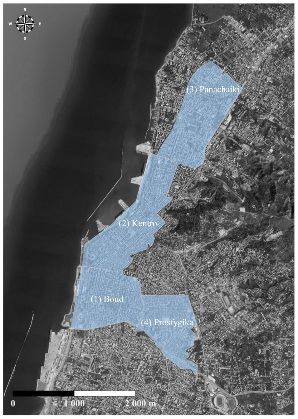
 [Green Version]
Figure 1. Map indicating the locations of the 4 largest PMAs of the City of Patras in western Greece.
Water 14 00098 g001
Figure 2. Water balance components as introduced by the International Water Association (IWA).
Water 14 00098 g002
Figure 3. Illustration of the three distinct regions characterizing the flow measurements in PMA “Kentro” on 6 December 2018, within the time frame from 00:00 a.m. to 06:00 a.m.: (a) 1-minute resolution timeseries, and (b) Their corresponding empirical probability density function (ePDF); see main text for details.
Water 14 00098 g003
Figure 4. Water balance analysis components in PMAs: (a) Boud, (b) Kentro, (c) Panachaiki and (d) Prosfygika, as obtained by applying the IWA top-down approach. PMA locations are illustrated in Figure 1.
Water 14 00098 g004
Table 1. Name, total area, length of the pipeline grid, population and number of authorized active hydrometers of the 4 largest pressure management areas (PMAs) of the city of Patras shown in Figure 1.
PMA Number and NameArea (m2)Pipeline Length (m)PopulationHydrometers
(1) Boud952,56844,95415,36210,586
(2) Kentro1,206,86762,17413,99216,454
(3) Panachaiki1,184,26251,70318,00311,983
(4) Prosfygika801,55743,24610,6575206
Table 2. Components of the water balance (or top-down) approach for the 4 PMAs of the WDN of the city of Patras, for the period from 1 November 2018 to 28 February 2019 (i.e., 119 days): SIV (system input volume), BAC (billed authorized consumption), NRW (non-revenue water), UAC (unbilled authorized consumption), WL (water losses), AL (apparent losses), RL (real losses). PMA locations are illustrated in Figure 1.
PMA Number
and Name
SIV
(m3)
BAC (m3)NRW (m3)UAC (m3)WL (m3)AL
(m3)
RL
(m3)
(1) Boud638,400344,379294,02063,840230,18034,438195,742
(2) Kentro467,134154,056313,07846,713266,36515,406250,959
(3) Panachaiki1,210,274457,614752,660121,027631,63245,761585,871
(4) Prosfygika555,293262,232293,06255,529237,53226,223211,309
Table 3. Statistics of the minimum night flow (MNF) estimates obtained by applying Serafeim et al. [42] approach to the 4 PMAs of Patras WDN. μMNF and σMNF denote the ensemble mean and standard deviation of the individual MNF estimates obtained in different days of the low-consumption period from 1 November 2018 to 28 February 2019. PMA locations are illustrated in Figure 1.
PMA Number and NameμMNF
(L/s)
σMNF
(L/s)
95% Confidence Intervals
(L/s)
Lower LimitUpper Limit
(1) Boud26.680.5526.5826.78
(2) Kentro69.853.9169.1570.55
(3) Panachaiki18.812.2418.4119.21
(4) Prosfygika27.801.2727.5728.03
Table 4. Components of the minimum night flow (or bottom-up) approach for the 4 PMAs of the WDN of the city of Patras, using the 95%-confidence limits in Table 3. UNC, NNF, NDF and RL indicate the users’ night consumption, net night flow, night-day factor and real losses, respectively. The calculated volumes correspond to the period from 1 November 2018 to 28 February 2019 (i.e., 119 days). PMA locations are illustrated in Figure 1.
PMA Number and NameMNF 95% Lower [Upper] Limit (L/s)UNC Lower [Upper] Limit
(L/s)
NNF Lower [Upper] Limit
(L/s)
NDFRL Lower [Upper] Limit
(m3)
(1) Boud26.58 [26.78]4.414 [4.444]22.18 [22.34]24.00227,905 [229,653]
(2) Kentro69.15 [70.55]21.13 [21.55]48.02 [49.00]27.24561,231 [572,685]
(3) Panachaiki18.41 [19.21]0.500 [0.500]17.91 [18.71]24.12185,068 [193,334]
(4) Prosfygika27.57 [28.03]4.432 [4.500]23.14 [23.53]27.52272,817 [277,427]
Table 5. Average (over the whole period of MNF estimation, i.e., from 1 November 2018 to 28 February 2019) pressure set points during day (Ps,d, 06:00 a.m.–00:00 a.m.) and night (Ps,n, 00:00 a.m.–06:00 a.m.) hours. PMA locations are illustrated in Figure 1.
PMA Number and NamePs,d (atm)Ps,n (atm)
(1) Boud2.302.30
(2) Kentro3.063.54
(3) Panachaiki6.876.91
(4) Prosfygika3.393.96
Table 6. Estimates of real losses (RL) obtained using the water balance (WB) and MNF approaches, expressed as fractions of the system input volume (SIV). PMA locations are illustrated in Figure 1.
PMA Number and NameWB RL
(%)
MNF RL Low Limit
(%)
MNF RL Upper Limit
(%)
Absolute Relative Difference
(%)
(1) Boud38.0541.0441.367.28–7.99
(2) Kentro48.4146.3747.322.30–4.39
(3) Panachaiki30.6628.9930.281.25–5.77
(4) Prosfygika53.7258.4059.398.01–9.54
Publisher’s Note: MDPI stays neutral with regard to jurisdictional claims in published maps and institutional affiliations.

