1. Introduction
This paper is devoted to a 3D hydrodynamics and transport of polluted particulate matter resuspended from the bottom sediment in a long and narrow Canal (called Rove) in the frame of an old and complex engineering project of partial reopening of a collapsed tunnel (
Figure 1). The aim of this reopening project is the remediation of the bottom sediment of the Rove Canal. The project itself consists to pump marine water, with a given flow rate (runoff), from the Bay of Marseille, to create a forced convection along this long Canal, down to a Mediterranean lagoon, called the Etang de Berre [
1].
Due to the collapse of the Rove tunnel in 1963, the inflow of marine water was stopped, what created a source of pollution due to an almost permanent water stagnation in the Rove Canal. This stagnation creates a negative environmental impact for nautical activities (rowing, water-skiing, canoeing/kayaking) which are today developed in the Rove Canal.
In the perspective of such a reopening, a detailed analysis of the sediments characteristics has been carefully performed by [
2]. It pointed different alarming ecological and environmental problems due to a severe concentration of contaminants in the sediments of the Rove Canal, and an evident risk of a downstream contamination of the Etang de Berre (EB).
However, the selection of the runoff level is still controversial for different reasons, environmental and financial (see [
3]). Indeed, the effect of the local wind is sufficiently strong in this area to generate resuspension of bottom sediments, even for such narrow and shallow Canal [
4].
The present study was decided in this context. This paper is an extension of the study by [
4] devoted to modelling and numerical simulation of the 3D salinity, current distribution and bottom shear stress (
) in this Rove Canal. It was shown that even though the transverse dimensions of this Canal are not large the local winds create intensive bottom currents that can permit floc erosion and even surface erosion. Here, a sediment transport model is coupled with the model previously applied for the hydrodynamics [
4]. The goal is to study the dynamics of the muddy bed sediments resuspended by the wind, and to understand (i) how the properties of such sediments would be changed due to successive erosion, resuspension, redeposition events, and consolidation; (ii) how the suspended sediments would be transported downstream by the forced circulation of pumped marine water.
A coupled hydrodynamical-sediment transport model is described in
Section 3. In
Section 4, a preliminary validation of such a model is performed by using the detailed data of sediment cores measured by [
2]. Then, in
Section 5, several 24 h-scenarios are devoted to the simulation of sedimentary transport connected to the reopening project by considering two inflow rates (
= 3 and 6 m
/s), for various wind forcings, including two opposite directions (N-NW and S-SE) and different wind speeds in the range 12–20 m/s. Finally, in
Section 6, an evaluation of the cumulative and instant fluxes of suspended particulate matters to Etang de Berre, as a function of
, is realized for the two wind directions, at an intermediate wind speed of 15 m/s, for the 24 h-scenario.
2. Study Site
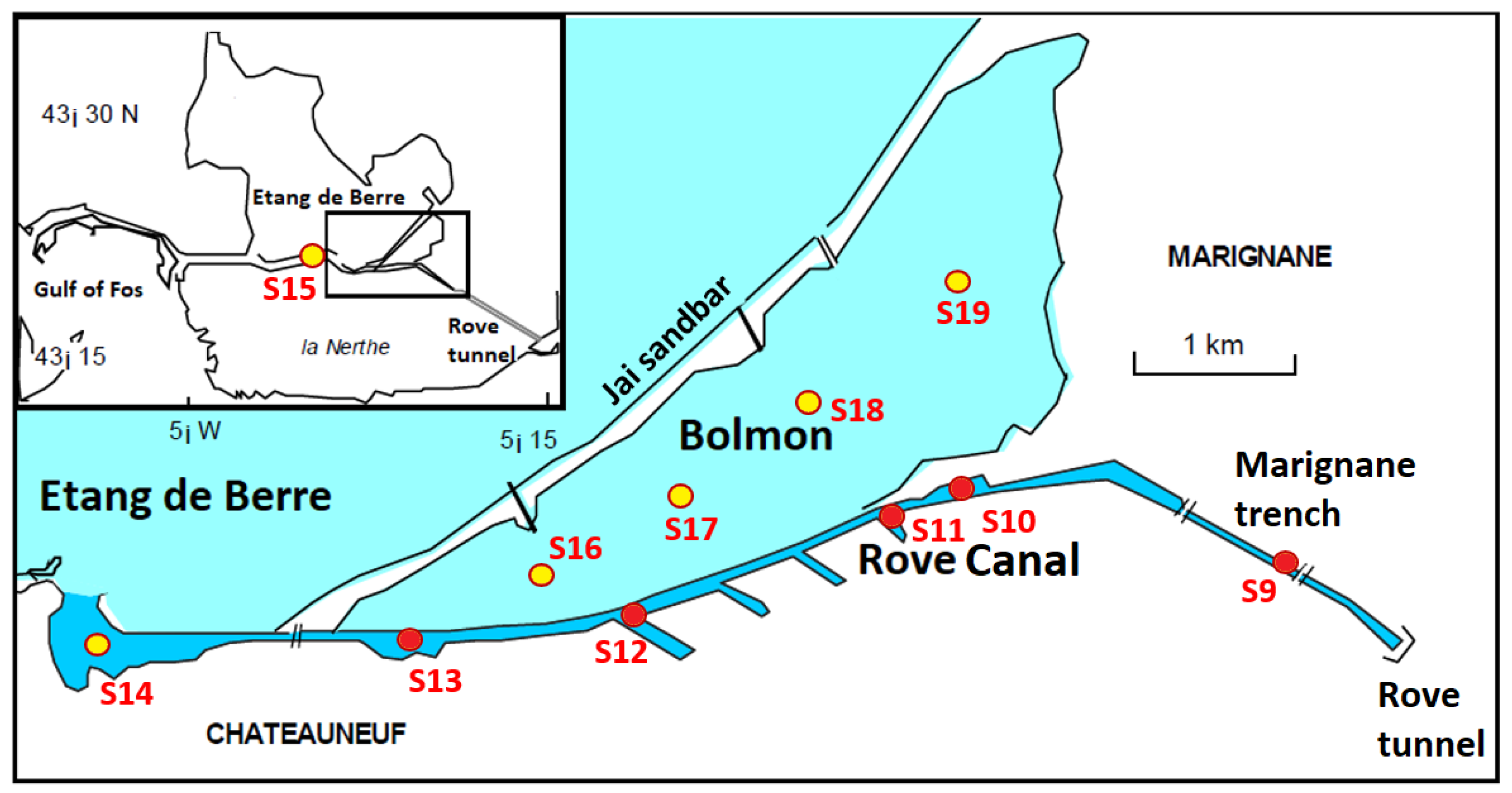
The Rove Canal (in the south of France) was opened in 1927 and was used (via a long sea tunnel) for freight shipments from the harbor of Marseille to Lyon through the wide brackish lagoon the Etang de Bere (EB), the Caronte Canal, Foss Bay and the Rhone River (
Figure 1). The tunnel was closed in 1963 after the section collapsed. This tunnel is 7 km long, 22 m wide, 15 m high and 4m deep. The Rove Canal, from the Rove Tunnel to EB, is 7.2 km long; the width varies (from 21 m to 70 m,
Figure 1). Nominal depth is 4.3 m.
As a result of the collapse of the tunnel, the water in the Rove Canal is practically stagnant, and the bottom sediments are seriously polluted. For this reason, for over 20 years there has always been a project to restore water circulation in the Rove Canal by pumping seawater from the Bay of Marseille through the Rove tunnel. This project is causing controversy regarding the mass flow rate to be pumped (on the order of 1–20 m/s) and the risk of transporting contaminated sediments downstream.
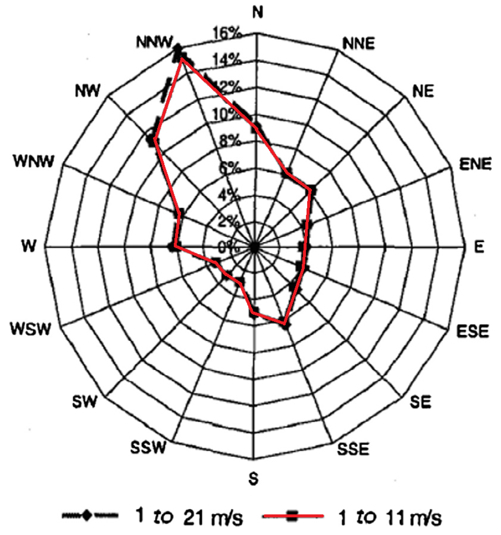
Another important feature of this site, is the occurrence of very frequent winds, in particular in the dominant direction: N-NW (see Figure 2).
The Rove Canal receives fresh water from a waste treatment plant (called the Palun) with a mean mass flow rate = 0.25 m/s.
As previously mentioned, in terms of assessing the environmental risks associated with the reopening project, [
2] conducted a detailed on-site experiment during periods of calm weather. In particular, this concerns the composition of bottom sediments (granulometry and pollutants) at various stations along the Rove Canal (
Figure 1). The composition of the sediments was measured in units of % fraction <2 mm at several stations (see Table 6a of [
2] for them); bottom sediments mainly consist of silt with a grain diameter of
d from 2
m to 63
m. Particular attention was paid to sediment sampling depending on the sampling depth, at which three sedimentary layers (strata) were analyzed: (i) strata1: unconsolidated silt (2 cm), (ii) strata 2: surface silt in compaction way (3 cm), (iii) strata 3: solid silt (under layer 2; several cm). On average, the Rove Canal deposits are mostly cohesive (78% silt and 6% clay); the remaining part being sand.
In addition, after [
2], the Rove Canal features heavily contaminated sediment characteristics. Physicochemical analysis of the concentration of the following pollutants revealed high concentrations of: (i) inorganic: Ca, Cu, Hg, Pb and Zn; and (ii) organic: PAHs (fluoranthene and benzo (a) pyrene), PCBs (CB 153) and TBT. Their Table 6a,b show that Cd, Hg, As, PAH, PCB and TBT contamination has been confirmed in the Rove Tunnel North sector, and this contamination persists in the Rove Channel with Cd, Hg and PCB. The risk associated with these deposits is presented in Table 7a of [
2]. In addition, the ecotoxicity has been shown to be very high in the Rove Tunnel (HCT and Cd) and in the Rove Canal.
The fine sediment fraction (silt and clay) that predominates in the Rove Canal is the one that preferentially captures the pollutants. Thus, an increase in the Rove Canal mass flow rate would increase the risk of downstream transport of suspended solids. Indeed, anthropogenic organic pollutants and metals carried by these particles are considered to be a serious health threat. Thus, it is important to estimate the amount of suspended solids transported to the Etang de Bere (EB) as a function of the forced mass flow (runoff).
3. Materials and Methods
Herein, a sediment transport model is coupled with the hydrodynamical model previously applied by [
4], under two different forcings: strong wind and forced seawater inflow. The main equations and features of the sediment transport model have been detailed by [
5,
6,
7]. All coupled model runs have been performed on the Aix-Marseille Computing Center. Typically, one scenario of 24 h with a time-step of 2 s, consumes 96 min of real time in parallel mode (using 32 nodes).
3.1. Hydrodynamics
We use the 3D model of hydrodynamics MARS3D (Model for Applications at Regional Scales) developed by the French Research Institute IFREMER ([
8,
9]). Detailed information about MARS3D model: governing equations, boundary conditions, and model discretisation can be seen in the previous work by [
4]. MARS3D is based on the incompressible Reynolds Averaged Navier-Stokes (RANS) equations in the classical Boussinesq approximation with the hydrostatic assumption.
For the present numerical simulation, we consider the Canal bathymetry obtained by [
10] by using a reconstruction method from the map given by [
11] from echo-sounding. The computational domain involves the part of Canal between stations S9 and S13. It spreads from 43.410524
N to 43.397576
N in latitude (x-direction, oriented West to East), and 5.210786
E to 5.141542
E in longitude (y-direction, oriented South to North), with a uniform horizontal resolution of 4 m (i.e., 1400 × 360 horizontal grid points; staggered C grid, [
12]). In order to more easily follow the variation of the surface elevation, a transformed vertical coordinate,
, is used in such a way that
at the surface and
at the bottom. In addition, to better take into account the two boundary layers (at the surface, and at the bottom) a refinement of the
grid is used, as in [
13] for the Etang de Berre.
3.2. Boundary and Initial Conditions
The model involves the horizontal components of the shear stress at the surface and the friction at the bottom. We use the following laws [
4]:
for the surface stress components
where
is the wind velocity 10 m above surface,
kg/m
is the air density,
is the surface drag coefficient which depends on the wind speed and the surface roughness [
14].
for the bottom stress components
with
where
is the velocity vector with horizontal components
,
is the bottom drag coefficient,
is the Von Karman constant,
is the reference density,
is the bottom roughness. The bottom boundary condition depends on the bottom roughness
which is connected to the grain size of the bottom sediments and will be further evaluated in the
Section 3.3.1 at the basis of the sediment core samples measured by [
2].
At the confluence of the Rove Canal with EB (at the western end of the Canal), we consider an open boundary condition.
In
Section 4 which corresponds to the present configuration (without reopening), we take into account the contribution of the Palun waste water treatment plant with the runoff
of 0.25 m
/s, and the contribution of a micro-tide which can reach about 5 cm at the junction of the Rove Canal to EB (according to [
1]). This micro-tide is simply expressed as:
where
denotes the initial time of computation,
A is the tidal period (about 44,714 s or 12 h 25 min).
In contrast, for the other model scenarios (after reopening) aimed to estimate the flux of suspended sediment matter to EB in the case of forced convection (
Section 5 and
Section 6), we neglect these micro-tide and Palun contributions. For these short scenarios (24 h), the salinity is assumed to be constant everywhere in the Canal (S = 20 PSU). We also neglect temperature heterogeneity; the numerical simulation is realized for a constant temperature (T = 20
C). The water density
was set to 1013.36 kg/m
(corresponding to T = 20
C and S = 20 PSU).
The wind rose of
(average daily wind speed at 10 m) provided by [
15] for the ten-years period 1992–2001 is used (
Figure 2) as in our previous paper concerning a very close area [
16]. It gives the mean annual frequency of wind speeds of 21 m/s and 11 m/s, in 16 directions. The dominant wind direction is N-NW, where the frequency of a wind speed of 11 m/s reaches 102 days per year. Thus, concerning the wind forcing, we will consider wind speeds
in the range 10–20 m/s in each of the two opposite wind directions (N-NW and S-SE).
3.3. Sediment Transport
For sediment transport, we use the MUSTANG sediment module (MUd and Sand TrAnsport modeliNG, [
5]) coupled with the MARS3D model, as well as provided by IFREMER ([
6,
17]). The MARS3D model manages the advection of particles in the water column in accordance with the three-dimensional structure, while the MUSTANG module controls the sedimentation of particles in the water column, as well as exchange with the layer through the processes of erosion, sedimentation and consolidation. In the MUSTANG module, processes such as sedimentation and erosion are modeled for each horizontal cell
separately (1D) with a variable number of layers, the thickness, porosity and concentration of which change over time due to sedimentation and resuspension events.
The modelling techniques in sediment transport simulations are split into two classes [
6]: (i) for non cohesive sediments (sand or gravel with high sedimentation velocity; which are not considered in this work), (ii) for fine sand and mud, which are mostly transported in suspension, an advection/diffusion equation is solved and the sediment evolution is straightforwardly deduced from both erosion and deposition rates.
Ref. [
6] described in detail a sediment transport modeling strategy that makes it possible to take into account: “simultaneous loading and transport of suspended sediments, mixing of several classes of sediments in the water column as well as in sediments, consolidation of silt and mixed sediment deposits with possible segregation of sand particles by adapting Gibson’s theory, controlling erosion flows depending on the cohesive or non-cohesive nature of surface deposits. Particular attention was paid to the method of renewing the content of sediment layers after deposition in order to simulate the possible filling of pores between coarse particles in the surface sediment before creating a new layer.”
The transport of suspended particles is computed by solving the advection-diffusion (
5) for the concentration of different particle classes assuming that sediment particles have the same velocity as water masses, except the vertical settling component:
where
C—sediment concentration in water,
—particle settling velocity,
—velocity components along coordinates
,
—coefficient of vertical turbulent exchange,
E—erosion flux and
D—deposition flux.
Equation (
5) involves sink and source terms at the bed boundary, which are deposition and erosion fluxes under conditions defined by the hydrodynamical regime and the characteristics of the both suspended and deposited sediments. This means that model requires the formulation of both erosion and deposition laws (described below).
The particle classes are grouped into three types defined by their behaviour [
6]:
“coarse type, generic for non-cohesive particles that are transported as bedload only: it is normally affected to coarse sand, and can be extended to gravels, cobbles and pebbles;
sand type, generic for non cohesive particles that are transported in suspension: it refers to fine sand, but also to medium sand, since the possibility to simulate transport capacities through an advection-diffusion process has been demonstrated [
18];
mud type, generic for cohesive particles; these are naturally transported in suspension, but are also likely to flocculate (inducing a variation of settling velocity) and to undergo consolidation in the bed; the mud type is usually affected to silt and clay, but could also be used for organic matter”.
MUSTANG model involves a pore filling procedure described by [
6]. The procedure starts with the filling of sedimentary layer by the coarser particles, such as gravels and sands, and then by the particles of mud type filling the spaces between the pores of the coarser particles until the critical concentration of the mixed sediment achieved. This pore filling procedure to obtain mixed mud-sand sediment is applied to an initial sediment column (with the respect of the given particle fractions) and then at each time step when sedimentary dynamics calculation is called for in the MARS3D.
As it is mentioned in [
6], the sediment erodibility in fluid-particle mixture depends on the volumetric concentration maximum, which corresponds to the volume of the chosen particle type divided by the total volume of the fluid-particle mixture; it is varying between 0 and 1. For the present study, this volumetric concentration has to be provided in MUSTANG for sorted sand and mud-sand sediments whatever the combination of particle types (see Figure 1 of [
6]).
In this work, the Rove Canal sediment is represented by 10 sediment sublayers.
3.3.1. Sediment Granulometry Data and Main Size Classes
A major difficulty for implementing the sediment transport model is the choice of the particles as a state variables, since natural size-spectra are continuous and the computation cost increases with the number of state variables.
Various measurements of sediments and suspended matter in the Rove Canal, tunnel and adjacent waters are given in a detailed report by [
2]. This report also contains an annexe with a spectral analysis on the sediment granulometry for the stations S9–S13. We assembled this raw data for the stations S9–S13 located within the studied area of the Canal and then performed a statistical analysis in order to identify the main particle size representatives, their fractions and also to carefully parameter MUSTANG module.
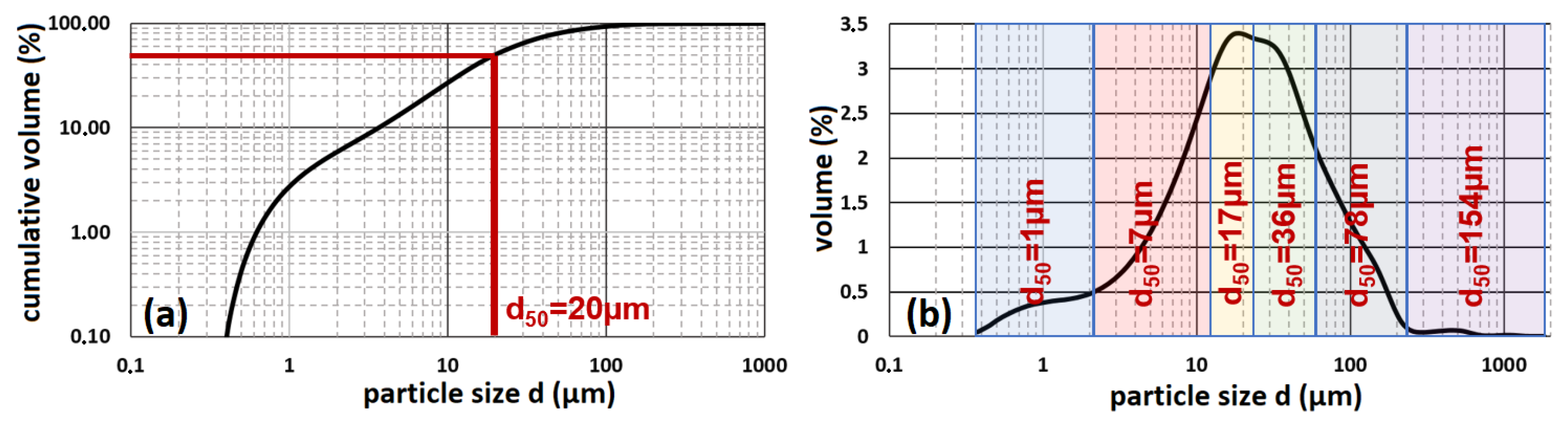
Figure 3a resumes a cumulative volume (%) per particle size for the mean over stations and strates sediment of the Rove Canal measured by [
2]. According to this figure the median diameter
m of all presented size classes corresponds to the medium silt. After Nikuradze formulation:
, such a
corresponds to
m.
We subdivide the mean sediment granulometry over stations and strata onto 6 particle size ranges (
Figure 3b) and then find the representative of each size class and its fraction for the sediment transport modelling (
Table 1).
The sediment characteristics (particle type, size range, particle size and initial fraction) used herein are given in
Table 1. They correspond to measurements performed by [
2]. Using these experiments, 6 particle sizes have been selected for our model (
Table 1) corresponding to 2 particle sizes of sand type, 3 particle sizes of mud type, and 1 particle size of clay type; i.e.,:
. Initial fractions in
Table 1 correspond to means over core samples, at the stations S9–S13.
In addition to the selection of sediment particles and their fractions, our model requires two values of volumetric concentration maximum: for pure sand and for the mixed sediment of the Rove Canal. Concerning the pure sand, a maximum value of 0.58 is used according to [
19] it was also chosen by [
6,
7]. Concerning the mixed sediment, we followed the soil classification triangle suggested by USDA (US department of Agriculture) which is based on the separate sand, separate silt and separate clay fractions [
20]. According to this classification, the mixed sediments in the Rove Canal correspond to the type called “silt loam”, with a maximum of the volumetric concentration of 0.5.
Concerning the sediment density, we take the option of the MUSTANG package in which the density of 2650 kg/m (corresponding to quartz) is used for all particle sizes.
3.3.2. Deposition
MUSTANG model involves a sedimentation process, which the formulation is given by [
6]. The general formulation for the sediment deposition flux follows Krone law:
where
is the deposition flux,
is the settling velocity,
is the concentration and
is the critical bottom shear stress for deposition for the particles of one size class with the grain diameter
.
As input parameters we need to provide settling velocities
of the different suspended sediment particles and their critical shear stresses for deposition
.
was estimated following [
21] formulation. For the four cohesive substances (silts and clay), the settling velocity is considered to be constant (i.e., we do not take into account a flocculation process) and has been estimated using the Stokes law (the maximal limit of settling velocity). For non-cohesive particles (sands), the settling velocity is taken from Soulsby formulation (after [
6,
22]).
Table 2 resumes input parameters needed to MUSTANG to simulate deposition process.
For the deposition process, if all sediment sublayers are filled up, MUSTANG model provides additional upper sublayers to be filled by settled particles.
3.3.3. Erosion
In MUSTANG model the erosion flux is based on the formulation from [
23] with erosion rate
E expressed as a function of the excess-shear stress to a power:
where
—the erosion rate constant,
—the critical bottom shear stress for erosion, and
n—the power law number.
MUSTANG erosion parametrization depends on the fraction of the cohesive sediment (mud). Three different regimes of erosion are considered: (i) the sediment behaves as non-cohesive sediment below a first critical mud fraction (
), so the prescribed erosion regime follows the formulation of pure sand erosion; (ii) above a second critical mud fraction (
, Ref. [
6]), a cohesive erosion behavior is defined; and (iii) for an intermediate content of mud (
) a transitional erosion behaviour of the mud-sand mixture is considered; and in this case an interpolation method of erosion rate is prescribed between non-cohesive and cohesive erosion rates
.
Ref. [
6] describes in detail such an erosion regimes, for which erosion rate constant
and power law number
n for pure sand and pure mud should be determined in accordance with the nature of modelled sediments. An interpolation function for
,
and
n should be chosen (among two specified) within MUSTANG (decreasing exponentially or linearly from value for pure sand to value for pure mud). In the model,
is determined for pure sand following the Shields criteria formulated by [
19]. While for pure mud, it is varying with the consolidation state of the sediment and follows a classical power law depending on mud concentration ([
6,
24]).
For the Rove Canal, typical values for the limits of pure sand and pure mud erosion behaviours have been chosen (
= 0.2 and
= 0.7) the same as in [
6,
25]. Power law number
n for the erosion equation Equation (
5) in the cases of the pure sand and pure mud have been also chosen the same as in [
6,
25] and equal to 1.5 and 1 respectively. Linear interpolation function between values of
,
n and
have been chosen for a transitional erosion behaviour (mixed mud/sand sediment case). Erosion rate
for pure sand was set to an experimental value of 5.94
kg·m
/s for 200
m grain size [
25]. For the pure mud, erosion rate
was set to 2
kg·m
/s—value taken from [
26] for surface erosion of muddy sediments.
3.3.4. Consolidation
The consolidation model follows the modeling strategy presented by [
6] then updated by [
27]. The consolidation model solves the Gibson equation for mixed sediments, taking into account the segregation processes, the permeability and the effective stress regimes of the sedimentation/consolidation phases [
27]. Ref. [
27] carried out the numerical modeling of the consolidation of mud-sand mixtures by considering the data of the experiments on a settling column. This version of the consolidation model has been shown to correctly simulate the sedimentation and consolidation processes for mixed sediments with moderate to high sand content (15 to 50%). Ref. [
27] presented a set of parameters that can produce a reasonable level of predictive accuracy for the consolidation of mixed sediments integrated into a 3D sediment transport model.
In this paper, we use the formulation for modeling the permeability process proposed by [
27]. It consists of a combination (minimum function) of two different formulations to calculate the permeability constitutive relationship. The first is related to the void ratio (e.g., [
6,
28]), and the second is related to the relative volume fraction of fine particles based on the fractal theory presented by [
29]. Among the numerous experimental data used to parameterize the permeability model presented by [
27], the experimental sample MSMB-C2 at Cancale Beach in the Bay of Mont Saint-Michel shows the greatest similarity to the Rove Canal sedimentary mixture, as it has a sand content of about 15%. Thus, we selected a set of individual parameters for MSMB-C2, detailed in Table 3 of [
27], with an estimated high predictive skill (
and
).
3.4. Wind-Driven Flows in a Transverse Section
The main driving mechanism considered in the present paper concerns the wind effect on the erosion of bottom sediment in the Rove Canal, in the most frequent wind direction which is almost perpendicular to the canal. It is interesting, that to permit a better understanding of the results given in
Section 5,
Section 6 and
Section 7, to provide a typical representation of the wind-driven flows (x- and y-components) in a transverse section of the Rove Canal. It is done in
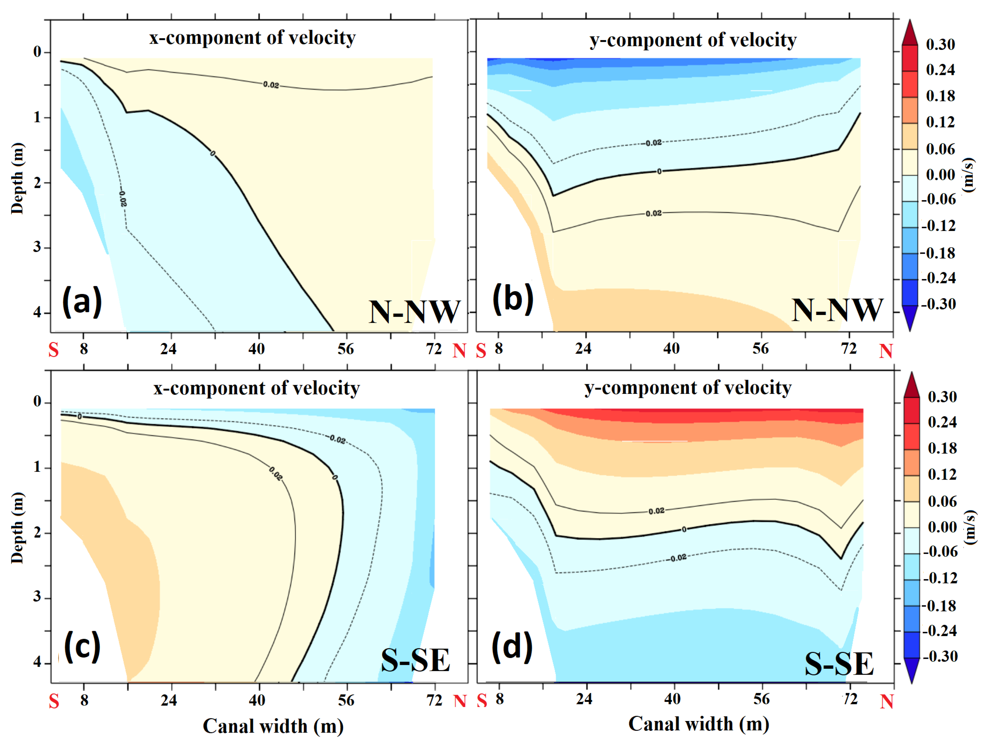
Figure 4 for a wind speed of 15 m/s, during the constant wind period and in absence of forced convection (
= 0).
From the x-component field of velocity, we can see a bidirectional flow in the longitudinal direction; straight lines correspond to the velocity from West to East, and dotted lines from East to West. For the y-component fields of velocity, we have a bidirectional flow in the transverse direction; straight lines correspond to the velocity from South to North, and dotted lines from North to South. The directions of each of both bidirectional flows are opposite for S-SE vs. N-NW direction.
Due to the fact that N-NW and S-SE directions are almost perpendicular to the canal, the transverse velocity is higher than the longitudinal one (one order of magnitude, for the maximum velocity).
4. Results: Validation Scenario
In this Section, we present a validation scenario aimed to control the ability of our model to represent correctly the process of sediment consolidation after a long windy period. It is based on the research work of [
27] which describes the consolidation process as the succession of three regimes. After these Authors, the consolidation process is driven by a pore water release: firstly without solid skeleton formation, named as the “permeability” regime, and secondly with solid skeleton formation named as the “effective stress” regime (e.g., Ref. [
30]). According to [
30] the typical duration of such a “permeability” regime is of about 10 days.
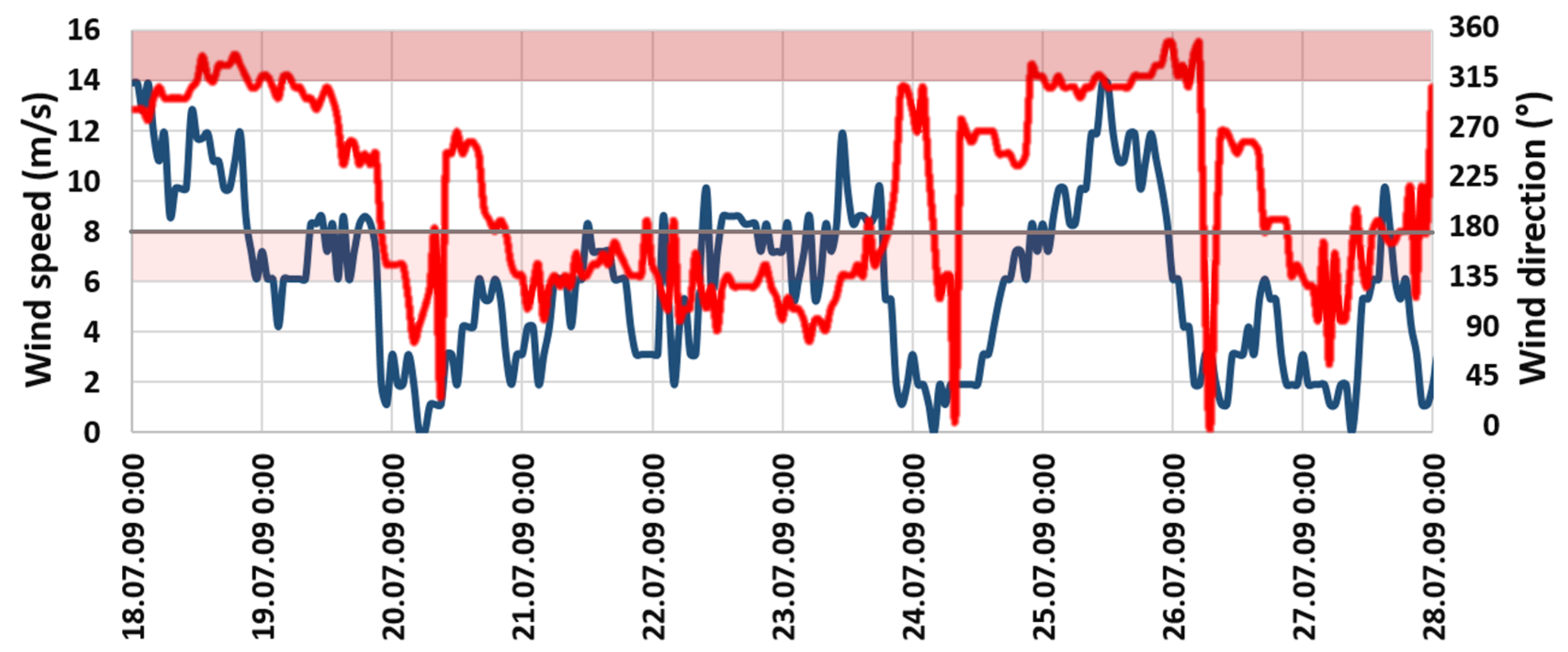
Our validation scenario concerns the simulation of the sedimentary dynamics in the Rove Canal during a period of 10–12 days preceding the date of extraction of sediment cores [
2] on 28 July 2009. For that period, the hourly wind data (intensity and direction), presented in
Figure 5, are provided by the METEOCIEL data base (ref.
https://www.meteociel.fr/ (accessed on 20 October 2021)). The goal is to compare the sediment composition predicted by our model at the end of 10 days of a windy period, with the experimental results obtained by [
2] on 28 July 2009, after this period.
4.1. Idra In Situ Measurements of Sediment Composition
Two types of measurements reported by [
2] are used for the model validation: dry density profile of sediment samples at stations S10–S12 and also dry density of the entire sample core at stations S10 and S12. Among different physical-chemical characteristics of the Rove sediment and water, dry sediment fractions per sediment strata have been measured. The main sediment classes present in the sediment cores: sands (>63
m), silts (2–63
m) and clays (<2
m) are listed in
Table 1. By considering that the gain density of particles of all size classes corresponds to the density of quartz (2650 kg/m
) we can estimate the sediment dry density for each strata and station by multiplying their values in
Table 1 by 26.5. These dry densities will be further compared to the modeled ones.
4.2. Description of the Validation Scenario
For our validation scenario, the wind conditions, for a period of 10 days in July 2009, are obtained from a METEOCIEL meteorological site. Thus, the validation scenario concerns the period of 18–28 July 2009. Two additional forcings are taken into account: a sinusoidal micro-tidal flux of 5 cm amplitude (Equation (
2)) and a Palun wastewater runoff of 0.25 m
/s.
Concerning the sediment, the scenario starts with homogeneous initial conditions similar to those mentioned by [
27] for a site containing 15% of sand (see their Table 1). It corresponds to the following initial conditions: a sediment height of 1m (before pore filling) and an initial concentration of sediment of about 200 kg/m
, respecting sediment fractions obtained from [
2] measurements (see their Table 1). After the starting procedure of pore filling at t = 0, the sediment thickness is reduced to 0.5 m.
Four additional variants have been tested: (a) with two initial sediment concentrations increased by +10% and decreased by −10% and (b) two durations increased by +1 day and reduced by −1 day, in order to check sediment sensibility to these parameters. These additional tests do not show significant influence on the sediment composition at the end of simulation (28 July).
Concerning the experimental data of IDRA to be compared with our numerical results, we have to note that the positions of the Stations S9–S13 are not exactly referenced, but they would be logically correspond to the center of the deepest part of the Canal (4 m). Accordingly, the numerical results are averaged over an area close to such central position of each station. This averaging is realized on a rectangular area with a length of 20 m (4 cells, along the Canal) and a width corresponding to all the deep part of the Canal (where H ≥ 4 m).
To exhibit the consolidation process, we followed IDRA approach by dividing sediment thickness in 3 strata as follows: the upper 2 cm are considered as strata-1, the next 3 cm as strata-2, and the remaining length as strata-3.
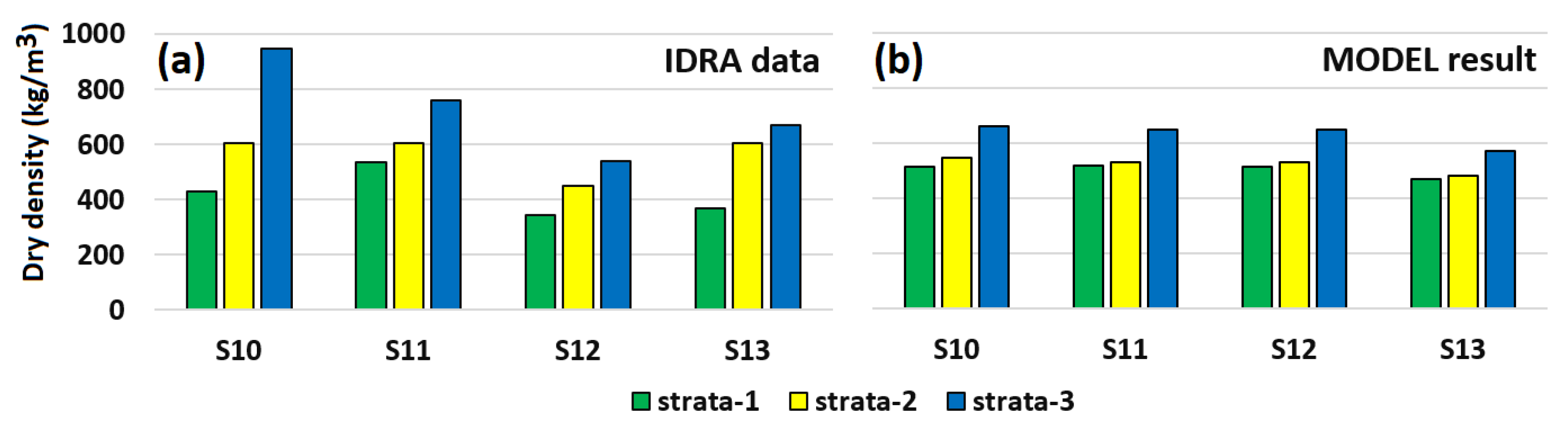
Figure 6 shows dry density distributions reported by IDRA in these 3 strata at S10–S13; the values are simply obtained by multiplying by 26.5 the % fractions listed in
Table 3. This
Figure 6 also compares these experimental results with those obtained at the end of our model scenario, on 28 July 2009.
The model results fairly well reproduce the consolidation of the lower strata. The experimental data reveal substantially higher variation of density from upper to lower layers. The difference between experimental and numerical results can be partly explained by the fact that the model is applied for a relatively short duration of wind stress, and it neglects other forcing processes due to the lack of information. From another side, some information about measurements is missing, such as the exact core sample thicknesses; e.g., a thicker strate-3 in the core could contain more consolidated sediment than in the model.
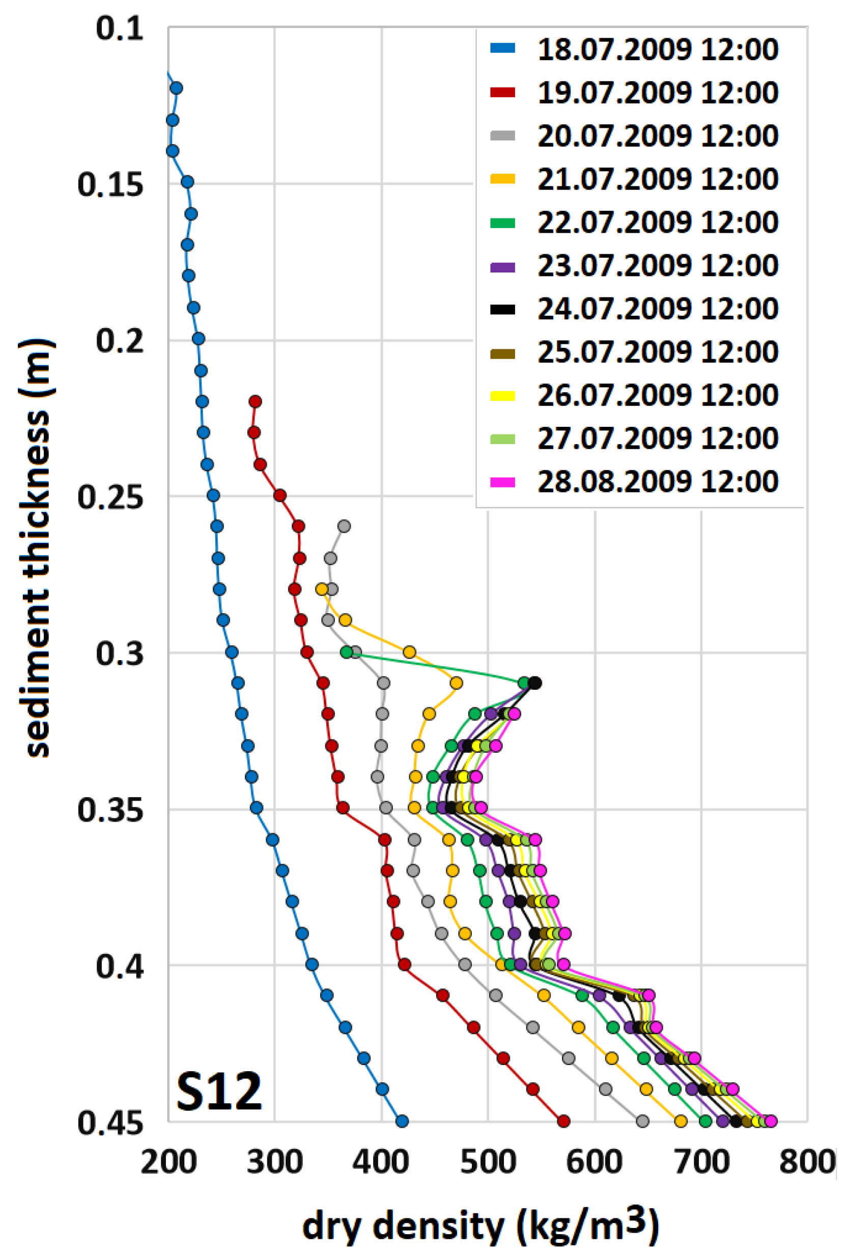
Figure 7 shows an example of sediment density evolution (consolidation) at S12 during the period of 10 days. During the first 5 days from 18 to 23 July, the variations of sediment thickness (reduction) and of density (increase) are fast (
Figure 7). The next days, the consolidation process decelerates (the changes in the entire sediment column became minimal): the level of sediment-water interface stabilizes and density continues to increase but very slightly. This behavior corresponds well to that described by [
27], with the duration of the permeability regime of about 10 days for their MSMB-C2 site (with a similar sediment type and composition).
It was not in our scope to considerably extend the duration of this scenario to reach a more accurate comparison, and the duration of ten days under the real wind sequence preceding the day of measurement permitted to understand that a period of about 10 days is necessary to reach a realistic sediment composition with an increase of consolidation from strata-1 (green column) to strata-3 (blue column).
For the next parts of our paper devoted to the effect of seawater runoff () on the flux of suspended sediment to EB, the sediment composition obtained at the end of this validation scenario will be used as the initial sediment composition all along the Canal.
5. Results: Resuspension, Erosion, Deposition and Consolidation along the Rove Canal under Wind Forcing and Forced Convection
After the model validation, we study the impact of the forced convection (
) and the wind forcing (separately and in combination) on the processes of erosion, resuspension, deposition and consolidation along the Rove Canal by using a set of 18 academic model scenarios of 24 h. These scenarios, called
, concern two main wind directions,
, three values of wind speed,
, and three values of tunnel runoff:
= 0, 3 and 6 m
/s. On the basis of our previous study in which the conditions for the onset of erosion in the Rove Canal were analyzed for the two wind directions, N-NW and S-SE [
4], we selected moderately-large values of the wind speed (around 15 m/s).
Here and in the next Section, we neglect micro-tide, Palun wastewater, salinity and temperature heterogeneity.
For the initial state of 3D velocity field in the Canal, we use the results obtained by the hydrodynamical model alone after 6 h of constant wind.
For the initial state of bottom sediments, we use the final state of the 10-days validation run (at 28 July 2009 12:00). This correspond to the 3D concentration fields of 6 sediment size classes and 2D sediment thickness field.
Each scenario starts with 8 h of a constant wind (with a wind speed large enough to generate resuspension), followed by a transition of two hours when the wind is completely slowing down, and finally a calm period (10–24 h) without wind. Such a sequence, with several hours of strong wind followed by a calm period (i.e., with wind lower than the critical condition for the erosion onset) is often locally observed, over a 10-year period [
15]. It is important to notice that the wind directions (N-NW and S-SE) considered in all scenarios are almost perpendicular to the Canal. As a consequence, for the first 8 h of all scenarios we obtain the strong dominance of the transverse velocity component compared to the longitudinal one (along the Canal, see
Figure 4). We can expect that the transverse component will have a dominant impact on the erosion/resuspension; while the longitudinal component will impact the downstream transport of the suspended sediments.
The aim is to analyze the evolution of 3D particle distributions in the water column and in the sediment, and also average (over Canal volume) matter stocks and fluxes (i.e., fluxes between water and sediment, and fluxes of matter transfer through the open boundary to EB leading to the downstream transport of absorbed contaminants).
The final goal is to obtain quantitative estimations of the transport to EB of suspended sediments, in particular the fines particles which are more attractive for the pollutants (silts and clay). The estimations will be useful for the engineers in charge of the ecological improvement of the Rove Canal ecosystem.
5.1. Evolution of SPM and of Dry Density of Sediment
In this subsection, we analyze the time evolution of suspended particulate matter (SPM, in kg), starting with the heterogeneous composition of bottom sediment obtained in the previous section (after 10-days of wind forcing for the period 18–29 July of 2009).
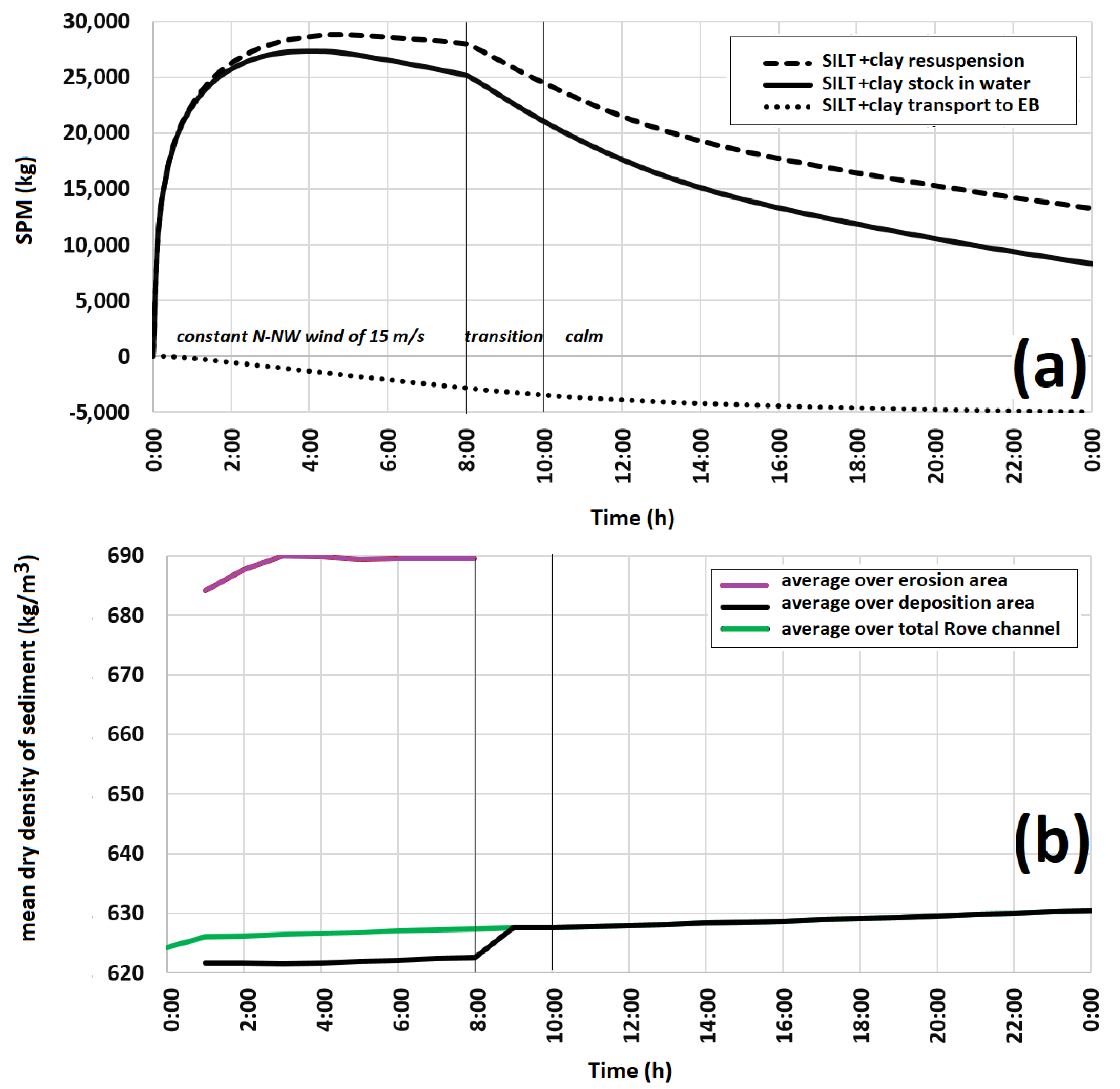
Figure 8a shows the time evolution of cumulative quantity of suspended particulate matter (SPM, in kg) in the water column of the entire Rove Canal. This quantity results from the balance between resuspension and sedimentation fluxes all along the canal. A part of this SPM quantity remains in the canal as a stock, and the complementary part corresponds to the cumulated flux to EB through the exit section of the Canal.
During the period of constant wind, the SPM quantity starts to increase due to resuspension, and then, it decreases slightly due to the sedimentation process (
Figure 8a). During this period, about 10% of the sediment particles resuspended in the entire Rove Canal moved towards EB (3000 kg vs. 27,000 kg). After this period, only the sedimentation process is active; silt particles are continuously settling, while the clay particles remain suspended; this sedimentation mechanism depends on the settling velocity that depends on the particle size (see
values in
Table 2).
Figure 8b contains three curves showing the evolution of a mean dry density of sediment for the reference scenario
(i.e., without forced convection). Two curves are given for erosion areas (when bottom shear stress is higher than the critical shear stress for erosion; i.e., for
) and for deposition areas (where
). An additional curve concerns mean over all the Rove Canal dry density of sediment (green line joining the black line after 9 h). This curve reveals a dominance of a continuous process of consolidation during the simulated period of 24 h (with and without wind). At the end of the simulated period of 24 h, the mean dry density is slightly increased by about 5 kg/m
due to the permanent consolidation process. During the first 8 h, dry density changes due to combination of two processes—erosion and consolidation; however, the impact of erosion on the mean dry density remains much lower compared to the consolidation (the results in
Figure 9, which show the surface of erosion areas compared to the total Rove Canal area, also confirm that).
Average sediment density over areas of erosion and deposition differ by about 60 kg/m
during the first 8 h of wind forcing. The highest density (of about 690 kg/m
) is found in the erosion areas. This high value can be compared, in our
Table 3, to the dry densities for the entire sample core measured by [
2] at S10 and S12: i.e., 446 and 661 kg/m
respectively in summer time, and 744 and 768 kg/m
in winter time where strong winds are more frequent.
5.2. 3D Sediment Fields (Erosion and Deposition Surfaces) for
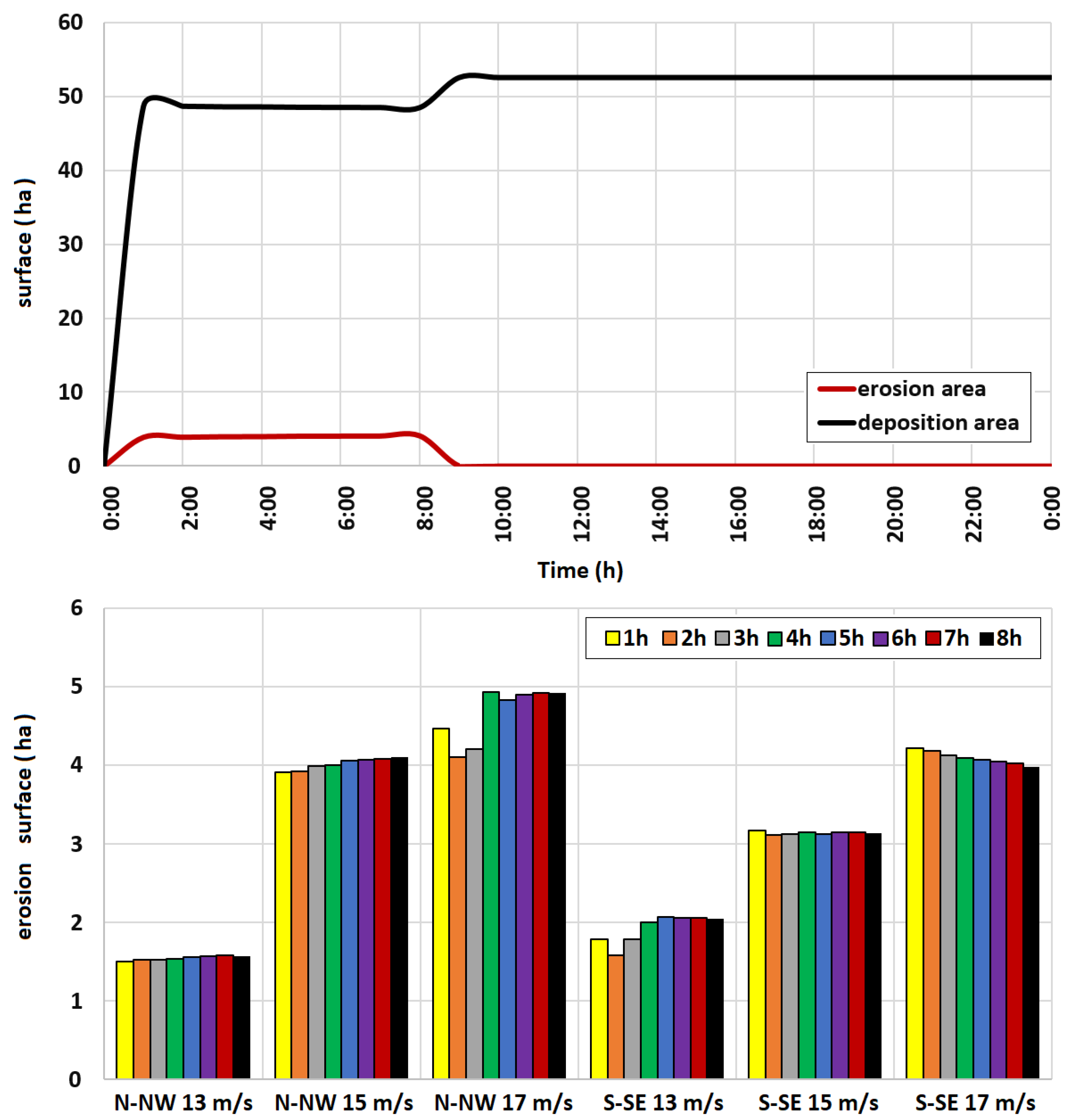
The characteristics of 3D sediment fields have been analyzed. It was found that even for strong wind conditions only a narrow part along the coastal area opposite to the wind direction has been eroded. Therefore, here we resume the wind impact in the form of simplified plots showing the evolution of erosion and deposition surfaces (m).
Figure 9a shows such an evolution for the scenario
; during the initial period of constant wind, erosion area (about 5 ha) is much lower than the deposition area (about 50 ha). Finally, after the wind slowing period, this erosion deposition area occupies entire surface of the modelled Canal (about 52.5 ha).
The increase of eroded area as a function of wind speed is shown in
Figure 9b for the two wind directions. It is more important for the N-NW direction; varying from 1.6 ha (for the wind speed of 13 m/s) to 5 ha (for the wind speed of 17 m/s) which remains a low percentage (3–9.5%) of the entire Rove Canal area. However, even such a low percentage of eroded area corresponds to quite a large resuspension flux of fine particles of silt and clay (up to 30,000 kg for a N-NW wind of 15 m/s,
Figure 8a). About 10% (up to 3000 kg,
Figure 8a at 8 h) of this suspended matter could leave the Rove Canal towards EB during the wind forcing, without any forced convection.
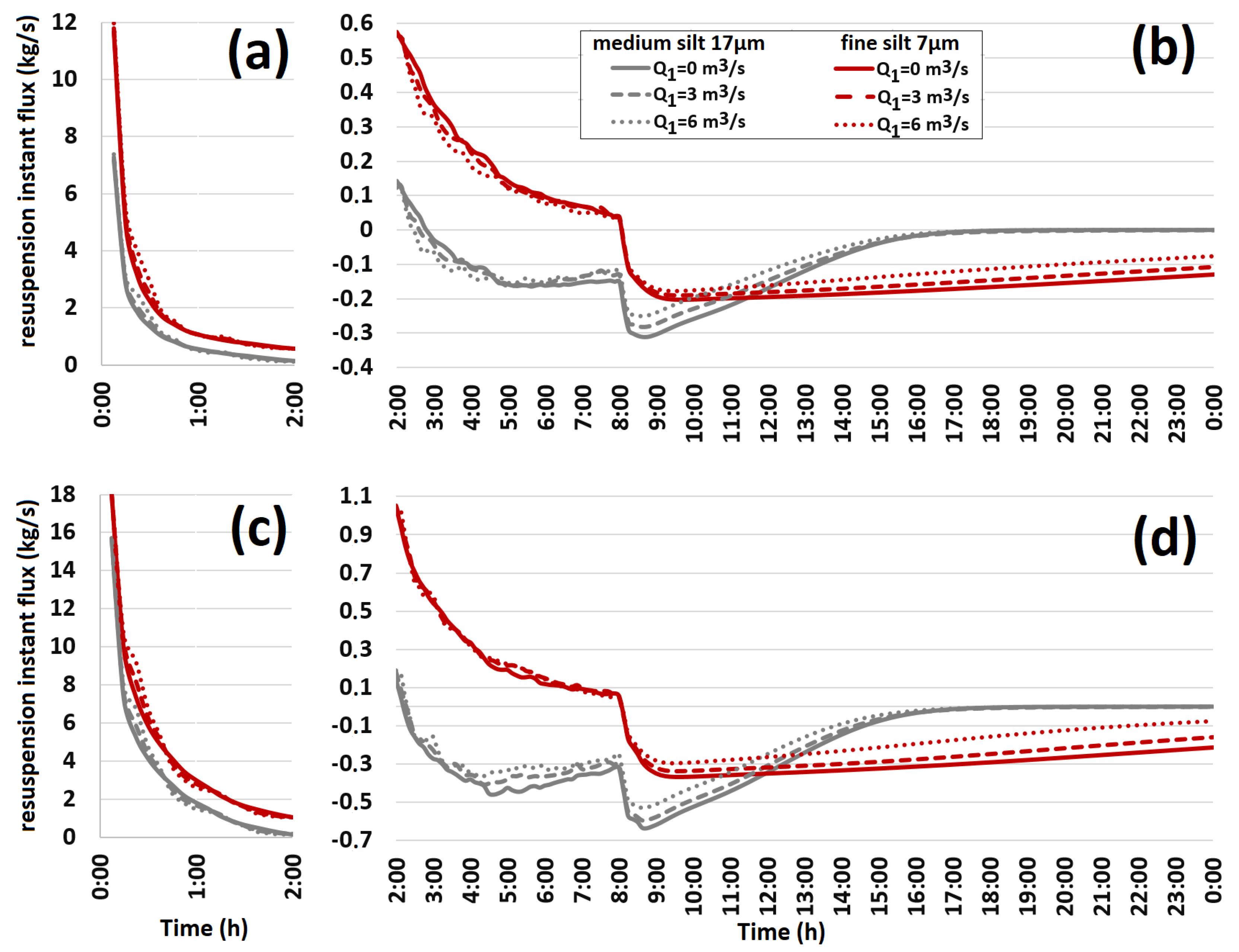
5.3. Instant Resuspension Fluxes of Medium and Fine Silts, as a Function of
The instant resuspension flux is positive and large at the beginning of the constant wind period; indicating that the flux from sediment to water due to erosion/resuspension is dominant (
Figure 10a,c). Then, this flux becomes rapidly negative, even before the end of the constant wind period, corresponding to a flux from water to sediment due to particle settling/deposition.
The effect of on this instant flux appears to be very weak during the period of constant wind (dotted and dashed lines are very close to solid lines).
The resuspension flux is higher for the S-SE wind (
Figure 10c); this is due to the fact that the initial sediment composition is the result of an initialization sequence of 10-days with the strong wind events in the opposite direction (N-NW). The medium silt particles (17
m) begin to settle down before the end of the wind forcing, after the first 2–3 h (
Figure 10b,d). In contrast, fine silt (7
m) is resuspended continuously during the whole period of wind forcing (0–8 h).
This behavior is consistent with those shown in
Figure 9a which shows that the cumulated resuspension flux presents an extremum before the end of the constant wind period.
After t = 8 h, the resuspension flux is always negative as the erosion mechanism stops (
Figure 10b,d). This sedimentation flux appears to be higher for the S-SE wind. For both wind directions, the medium silts (17
m) are fully deposited at about t = 18 h. In contrast, this sedimentation flux of the finer silts (7
m) continues to very slowly decrease. That means that a part of the fine silts and (of course of the clays) are still suspended more than 10 h after the end of the wind forcing, and even at the end of the 24 h-scenario. They will increase the SPM transport towards EB.
Compared to the reference case , an increase of leads to relatively low changes in resuspension flux during the constant wind period. On contrary, the influence of is larger in the period without wind. The instant sedimentation flux is reduced when is increased. So, the SPM stock in water is reduced and, correspondingly, the SPM transport towards EB is increased.
As the Rove Canal sediment is very contaminated, according to [
2], the next section is devoted to studying the effects of wind and forced convection on the SPM transport towards EB.
6. Results: Flux of Suspended Particulate Matter to Etang De Berre as a Function of for a Wind Speed of 15 m/s
This Section is devoted to estimate the SPM flux of the Rove sediment (contaminated) towards the confluencing ecosystem of the Etang de Berre (EB) which is already heavily eutrophied due to other reasons [
16].
In this Section (like in the previous section), we consider a wind scenario of 24 h with three successive periods: 0–8 h of constant wind, 8–10 h where the wind is slowing down, and 10–24 h without wind (called calm period).
This SPM flux will be further called OBC (open boundary condition) flux. It passes through the main open boundary at the western end of the Rove Canal, in connection with the EB. We will analyze two types of OBC fluxes-cumulative and instant. Cumulative OBC fluxes allow to estimate a quantity of matter (in kg) entering to the EB integrating all events of the scenario-wind, transition and calm. The instant OBC flux allows us to better distinguish one event from another; it assesses the quantity of matter per unit time at each instant.
In the next figures, only OBC fluxes of cohesive particles will be shown since they preferentially attract pollutants. In addition, the OBC fluxes for sand-particles are relatively negligible due to their high settling velocity; sand particles settle down to the sediment bed after a few minutes.
First, the reference scenario (with = 0) is considered. Then, two scenarios taking into account a forced convection (corresponding to the reopening project) will be considered with two flow rates ( = 3 and 6 m/s).
6.1. Reference Scenario ( = 0 and a Wind Speed of 15 m/s)
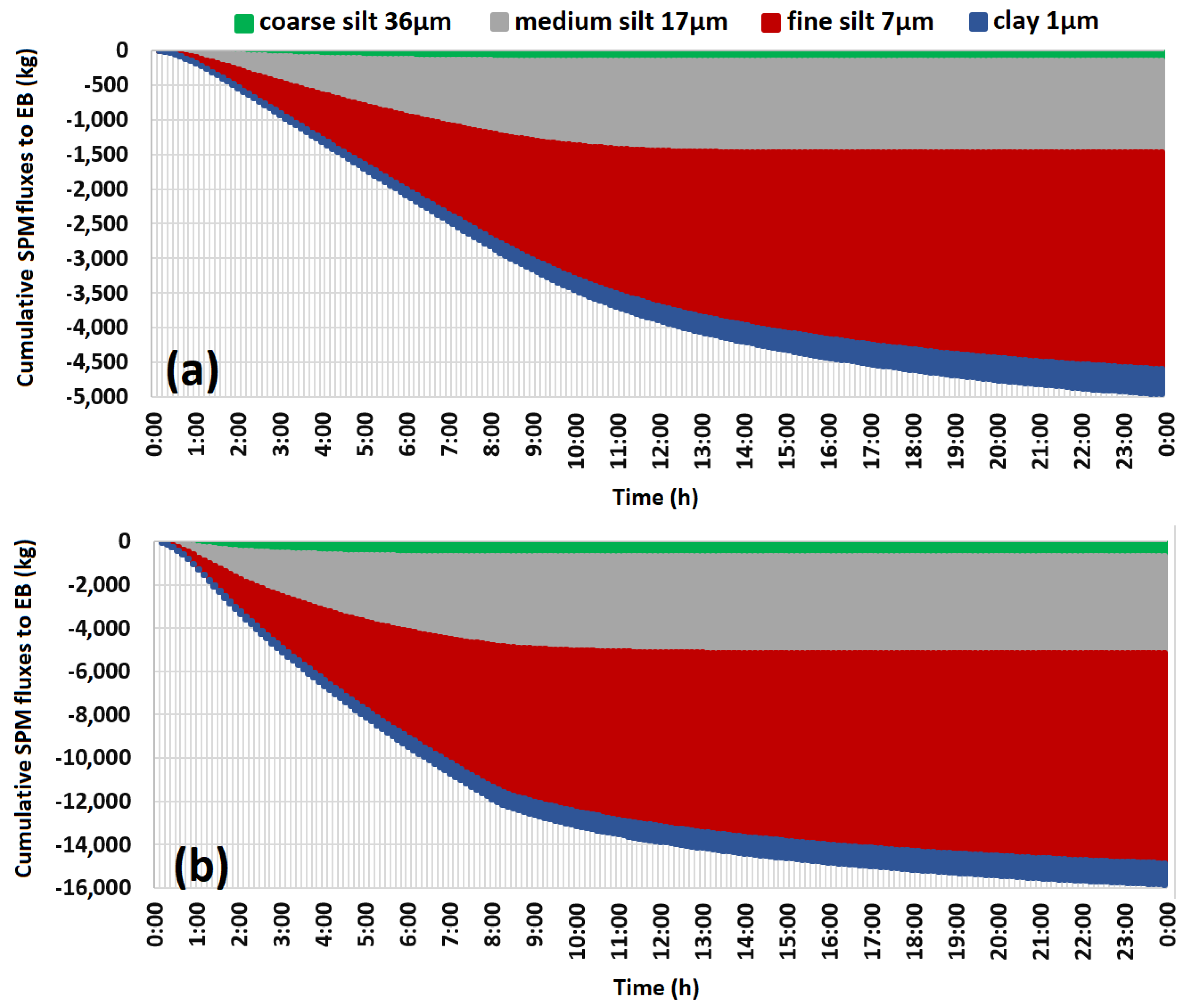
For the reference scenario (i.e., without any forced convection) the time evolution of the cumulated flux of SPM towards EB is presented in
Figure 11, for the four classes of finer sediments (clay and 3 silts). This flux continues to increase substantially after the windy period.
In fact, the open boundary condition at the exit section of the canal allows a bidirectional flow in the x-direction during the windy period. The x-component of the wind (along the canal) induces a current structure with a bidirectional exchange of water masses at this canal exit. For the N-NW direction, the water close to the southern side of the canal is coming towards EB and the water close to the opposite side has an opposite direction. In the case of the S-SE direction, the behavior is opposite; the water close to the northern side of the canal moves to EB, while the water close to the southern side moves from EB. In both cases, the water moving to EB contains suspended sediments (SPM) even without any forced convection = 0. Even when the wind stops, the bilateral motion of the water masses continues by inertia, increasing the SPM transport towards EB. For the S-SE wind, the flow velocity and its influence on the OBC flux are higher than that for the N-NW wind.
Figure 11 shows cumulative fluxes (in kg) per four cohesive particle types. As it was seen in the previous section (
Figure 10 for the resuspension and settling fluxes)—the impact of S-SE wind is higher compared to that of N-NW wind. In contrast with resuspention and settling fluxes (
Figure 10) where such a difference was about by a factor 2, the OBC fluxes difference of SPM to EB is higher (more than a factor 3); i.e.,: 16,000 kg against 5000 kg. The largest quantity of SPM coming to EB corresponds to the fine silt: about 3000 kg for the N-NW wind and 8000 kg for the S-SE wind; medium silt was found to be a little bit less abundant in OBC fluxes. These two particle sizes are initially more abundant in the Rove sediment (
Table 1). For the largest cohesive particles—coarse and medium silt, OBC cumulative fluxes increase only during the windy period (0–10 h), whereas for the finest (fine silt and clay) such fluxes continue to increase even after this period (during calm, 10–24 h). This means that these fine particles, due to their low settling velocity, continue to move (suspended in the water column) towards EB even after the wind stops. So, they could bring absorbed contaminants to EB even during the calm period.
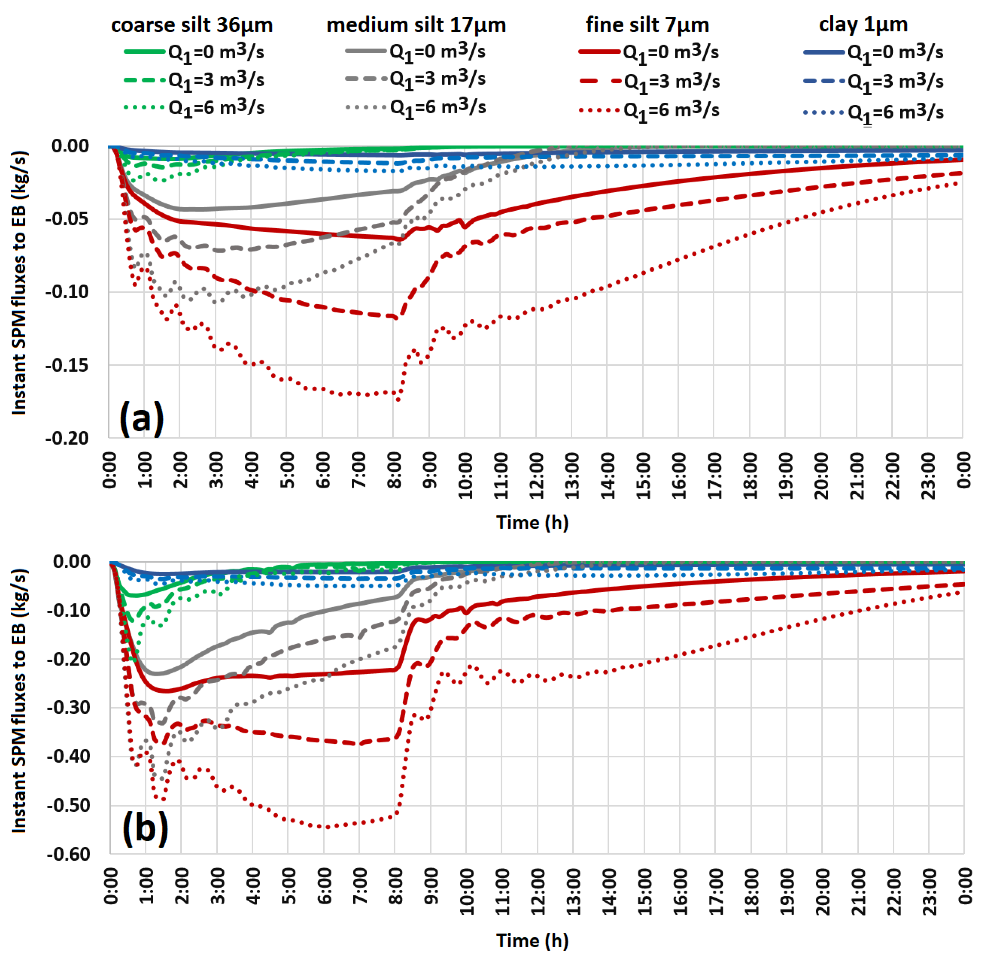
6.2. Instant OBC flux
Figure 12 shows instant OBC fluxes towards EB for four cohesive particles for the wind of 15 m/s in two directions (N-NW—
Figure 12a, and S-SE—
Figure 12b) and for three values of the tunnel runoff (0, 3 and 6 m
/s). Instant fluxes for the N-NW wind are 3–4 times lower that for the S-SE case. An increase of the seawater runoff by 3 m
/s induces an increase of instant fluxes of fine silts up by about 0.05 kg/s for the N-NW wind, and up by about 0.15 kg/s—in the S-SE case. After the windy period, OBC fluxes rapidly reduce to 0 for the medium silt, while they slowly continue to reduce for fine silt. For clay particles, OBC instant fluxes stay constant until the end (24 h). So, it is clear that OBC fluxes of particles of different properties (size, cohesiveness, settlement velocity, etc) will behave very differently during the windy and the calm periods of each scenario. In addition, we can see how OBC fluxes are strongly enhanced by the forced convection
.
6.3. Cumulative Obc Flux during a 24 h Scenario
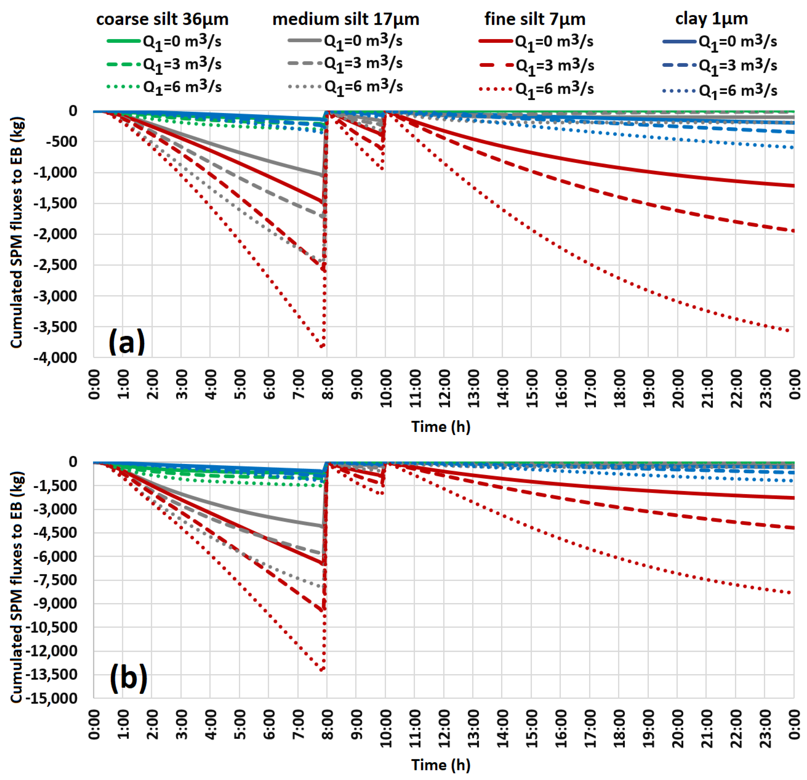
In order to better assess the quantity of matter leaving the Rove Canal towards EB, we calculated the cumulative OBC fluxes for each of the three periods separately (constant wind, wind slowing down, and calm). At the end of each period, the counter of the OBC cumulative fluxes is set to zero.
Figure 13 shows that, during the period of constant wind (of 8 h), the medium and fine silts are resuspended and transported to EB: (i) 1500–3700 kg of fine silt and 1000–2500 kg of medium silt—for the N-NW wind, and (ii) 6200–13,500 kg of fine silt and 4300–7600 kg of medium silt—for the S-SE wind. In contrast, during the calm period (10–24 h), only the finest particles stay resuspended and transported towards EB—in majority the fine silt (and much less the clay): (i) 1300–3500 kg of fine silt and 250–600 kg of clay for N-NW wind (
Figure 13a), and (ii) 2200–8200 kg of fine silt and 150–1250 kg of clay for S-SE wind (
Figure 13b).
The total flux to EB of the six SPM classes, for the windy and calm periods separately, is given in
Table 4, for the three values of
, for the wind speed of 15 m/s.
6.4. Transport of Contaminants to Eb
It is not in the scope of the present paper to model the transport of contaminants to EB. Nevertheless, it is interesting to mention that an evaluation of the contamination level is given by [
2] for 5 main contaminants: Cd, Cu, Me, CB153, PCBs (see their Table 6a,b for the strata of each sediment core at stations S10–S13 in the Rove Canal). By using these data, estimations of minimal, maximal and mean contamination levels (expressed in mg per kg of dry sediment) over three strata, for the stations S10–S13 are given in
Table 5. The highest contamination level appears for Cd and CB153.
The fine fraction of the sediments preferentially fixes the contamination [
2]. Fine particles in cohesive sediments are subjected to forces of attraction and repulsion, the result of which is the more or less marked capacity for aggregation (flocculation). The bond’s strengths are greater the greater the surface area to volume ratio, that is, when the particles are fine (less than 63
m, in particular). Despite some uncertainty, estimations of minimal and maximal contamination level are given in
Table 5 in order to allow the possible risk assessment of the contaminant moved with SPM towards EB.
The quantity of contaminant moved towards EB, can be evaluated from the contaminant level given in
Table 5 and from the total SPM flux shown in
Table 4. For the dominant N-NW wind, the total SPM flux is almost doubled during the wind period compared to the calm period. For the opposite S-SE wind direction, the total SPM flux is 5–6 times higher during the wind period than during the calm period. A similar behavior can be expected for the contaminants absorbed by SPM and moved to EB.
Considering the large amount of sediments suspended by the wind and transported to EB, it is clear that such an evaluation of the amount of contaminants transferred to EB would be needed before any attempt to reopen the Rove tunnel.
7. Discussion
Different scenarios have been investigated to evaluate the wind influence on erosion and transport of contaminated muddy sediments in a narrow and shallow canal. They use and complement a detailed analysis of the bottom sediments experimentally realized by [
2] in the reopening eventuality of a marine tunnel which collapsed 60 years ago.
The present analysis is important to evaluate the downstream contamination of a wide Mediterranean lagoon (EB), since the detailed experiments by [
2] demonstrate that the bottom sediments, which are mainly muddy, are highly contaminated. For that, the wind effect on the time evolution of complex sedimentary mechanisms of erosion/resuspension, deposition and consolidation has been performed, and, then, the downstream transport of suspended particles has been evaluated along the canal. This permitted us to evaluate the flux of such suspensions towards the lagoon through the canal exit, and evaluate how this flux is increased by a forced convection created by pumping devices added at the canal entrance.
Two coupled 3D hydrodynamical and sediment transport models (MARS3D/MUSTANG) have been presented in
Section 3. The sedimentary model is parameterized and calibrated for the Rove canal by using the data concerning sediment samples obtained by [
2]. For that, a distribution (%volume) has been proposed into six granulometric classes (1 clay, 3 silts, 2 sands).
In
Section 4, a validation scenario for a period of 12 days has revealed the importance of the consolidation of the freshly deposited sediment on the first days after deposition (
Figure 7), which is in accordance with other studies performed for the cohesive sediment of a similar composition by [
27].
In
Section 5, eighteen 24 h-scenarios with different wind forcings and forced convection permitted to give a quantitative understanding of the impact of each forcing on erosion and transport of muddy and cohesive sediments; the erosion being due to the wind and the transport being mainly due to the forced convection. Each 24 h-scenario involves a succession of three periods: constant wind (8 h), followed by wind slowing and calm weather. Our study permitted us mainly to analyze the time evolution of the dry density of bottom sediment, and of the suspended sediments during each of the three periods. It permitted to evaluate the dry density evolution in the areas of erosion and deposition. Concerning suspended sediments, the presentation of our results is limited to the finest ones (clay + silts) which would play the main role for the contamination risk: they concern the time evolution of resuspension flux, stock in the water column and flux towards EB through the canal exit. It is shown that the flux of suspensions to EB continue for several hours after the wind stops, even in the case
= 0.
Finally, for a wind speed of 15 m/s,
Section 6 provides the instant and cumulative fluxes towards EB of the suspended particulate matter (OBC flux, through the canal exit) which is directly associated to the risk of downstream contamination. Time evolution of these fluxes is presented for each of the finest sediment classes (clay and 3 silts), for the three values of
and for the two wind directions, during the three successive periods of the 24 h-scenario. The fine silt class (around 7
m) presents fluxes which are dominant. Indeed, this class corresponds to lower settling velocity than the other silts, whereas it is more abundant than the clay class. It is remarkable that during the calm period the instant flux decreases very slowly. The cumulated flux is presented for each of three periods of the 24 h-scenario. The part corresponding to the first 8h of constant wind is dominant, but the part corresponding to the following periods is significant, mainly for the N-NW wind.
As the two wind directions (N-NW and S-SE) are almost perpendicular to the canal, the longitudinal velocity component (along the canal) is much lower than the transverse one (
Figure 4). The transverse velocity component is responsible of the resuspension process while the longitudinal component is responsible of SPM transport towards EB (OBC flux). The increase of the forced convection contribute to the increase of the longitudinal component, reinforcing the SPM transport towards EB.
8. Conclusions
The present study brings new knowledge about the wind stress on erosion, transport, sedimentation and consolidation of muddy bottom sediments in a shallow and narrow canal. This was done for different 24 h-scenarios corresponding to two wind directions almost perpendicular to the canal and for large enough wind speeds; each scenario started with a period of constant wind (8 h), followed a period of calm weather.
At the beginning of each scenario of N-NW wind, a resuspension mechanism dominates all along the southern side of the canal; while a sedimentation is observed along the northern side. The simulation permitted to determine the extent of both erosion and sedimentation areas, as well as the density evolution of bottom sediment.
The SPM flux of erosion (from bed to water) is rapidly balanced by a sedimentation flux (from water to bed); e.g., after about 4 h of a wind speed of 15 m/s, for clay and silts. This is probably due to a consolidation process of bottom sediment, connected to the increase of dry density in the erosion area (e.g.,
Figure 9b).
For the opposite wind direction (S-SE), in contrast, the resuspension mechanism dominates all along the northern side of the canal, while a sedimentation is observed along the southern side.
The main findings, which concern the evaluation of the cumulated flux of clay and silts through the exit section of the canal, can be summarized as follows:
during the wind period, major flux comes from fine and medium silts (the most abundant classes);
after the wind period, major flux comes from clay and fine silt (the finest classes); the cumulated flux during 16h after the wind period is comparable with that during wind stress of 8 h;
a substantial flux exists even for ;
an evaluation of the flux increase in terms of the forced convection
has been provided for clay and silt classes (
Figure 13);
a preliminary evaluation of contaminant transport to EB as a function of
has been provided in
Section 6.4.
So, if the engineering project of reopening the Rove tunnel is maintained, it will be necessary to carefully extend the present study, to evaluate OBC flux for long periods and for real meteorological conditions. Indeed, the resuspension process would also occur for most of the other wind directions not considered in our simplified scenarios, but seen in [
16] and
Figure 2. For each wind direction, a contribution to such an OBC flux is expected as soon as the wind speed will overpass the threshold condition; with a resuspension flux which would increase with the fetch distance. Furthermore, it would be useful to account for salinity and temperature effects, and subsequently for other processes in suspended sediments, like the flocculation. All such improvements would be possible by using MUSTANG software; but at the conditions to get an evaluation of the needed physico-chemical constants for all interactions between suspended particles (including the organic matter and pollutants found in the Rove canal by [
2]).
Concerning the future scope of the present paper, we expect that our work will provide useful guide for scientists in charge of similar narrow and shallow coastal hydrosystems. At least, they should remember about wind influence on resuspension. For that, it will be always useful, according to priorities, to determine the threshold of sediments resuspension as a function of the wind and of the granular characteristics of the bottom sediments.
Author Contributions
E.A. contributed to conceptualization, methodology, investigation, validation, visualisation, paper writing. B.R. contributed to conceptualization, methodology, investigation, supervision, project administration, funding acquisition, and paper writing. K.K. contributed to investigation, software, visualisation, and paper revision and editing. All authors have read and agreed to the published version of the manuscript.
Funding
This research was funded by Agence de l’Eau-RMC—convention N 2010-0042 (in 2010) and the French Ministry of Foreign Affairs (ARCUS-Russia program, 2010) and Ministry of Education and Science of the Russian Federation (Minobrnauka)—075-15-2021-946. Centre de Calcul Intensif d’Aix-Marseille is acknowledged for granting access to its high performance computing resources.
Institutional Review Board Statement
Not applicable.
Informed Consent Statement
Not applicable.
Acknowledgments
We acknowledge financial supports by the French Water Agency (Agence de l’Eau-RMC—convention N 2010-0042 (in 2010), the French Ministry of Foreign Affairs ARCUS-Russia program, in 2010) and Ministry of Education and Science of the Russian Federation (Minobrnauka)—075-15-2021-946. Centre de Calcul Intensif d’Aix-Marseille is acknowledged for granting access to its high performance computing resources.
Conflicts of Interest
The authors declare no conflict of interest.
Abbreviations
The following abbreviations are used in this manuscript:
| EB | Etang de Berre |
| MARS3D | Model for Applications at Regional Scale |
| MUSTANG | MUd and Sand TrAnsport modelliNg |
| OBC | Open Boundary Condition |
References
- Ramade, A. Ouverture du Tunnel du Rove: Incidence sur les Échanges Hydraulique; Report Ramade-GERIM (August 1997); Port Autonome de Marseille: Marseille, France, 1997. [Google Scholar]
- IDRA Environnement. Etude de risque associé aux sédiments dans le cadre de la réouverture expérimentale du tunnel du Rove. Rapp. GPMM 2011, S90301, 318. Available online: https://letangnouveau.files.wordpress.com/2012/04/idra-etuderovevfinale16022011-2.pdf (accessed on 21 November 2021).
- Abrial, B.; Hucher, D. Expertise sur le Projet de Réouverture du Tunnel du Rove à Lcirculation d’eau de mer; Rapport No. 011009-01. Ministère de l’Environnement de l’Energie et de la Mer: Paris, France, 2017. Available online: http://www.ladocumentationfrancaise.fr/var/storage/rapports-publics/174000457.pdf (accessed on 20 October 2021).
- Alekseenko, E.; Roux, B. Risk of wind-driven resuspension and transport of contaminated sedimentsin a narrow marine channel confluencing a wide lagoon. Estuar. Coast. Shelf Sci. 2020, 237, 106649. [Google Scholar]
- Diaz, M.; Grasso, F.; Le Hir, P.; Sottolichio, A.; Caillaud, M.; Thouvenin, B. Modeling mud and sand transfers between a macrotidal estuary and the continental shelf: Influence of the sediment-transport parameterization. J. Geophys. Res. Oceans 2020, 125, e2019JC015643. [Google Scholar] [CrossRef]
- Le Hir, P.; Cayocca, F.; Waeles, B. Dynamics of sand and mud mixtures: A multiprocess-based modelling strategy. Cont. Shelf Res. 2011, 31, S135–S149. [Google Scholar] [CrossRef] [Green Version]
- Mengual, B.; Le Hir, P.; Cayocca, F.; Garlan, T. Modelling fine sediment dynamics: Towards a common erosion law for fine sand, mud and mixtures. Water 2017, 9, 564. [Google Scholar] [CrossRef] [Green Version]
- Lazure, P.; Dumas, F. An external-internal mode coupling for a 3D hydrodynamical model for applications at regional scale (MARS). Adv. Wat. Res. 2008, 31, 233–250. [Google Scholar] [CrossRef]
- Lazure, P.; Garnier, V.; Dumas, F.; Herry, C.; Chifflet, M. Development of a hydrodynamic model of the Bay of Biscay. Validation of hydrology. Cont. Shelf Res. 2009, 29, 985–997. [Google Scholar] [CrossRef] [Green Version]
- Sukhinov, A.I.; Sukhinov, A.A.; Roux, B. Reconstruction of Basin Bottom Surface for High Precision Hydrodynamics Modeling Using Parallel Computations. In International Conference on Parallel Computational Fluid Dynamics (Parallel CFD 2007); Elsevier: New York, NY, USA; Paris, France; Tokyo, Japan, 2008; 8p. [Google Scholar]
- Pont, D.; Barroin, G. Expertise Écologique de L’éTang de Bolmon en vue de sa Réhabilitation; Rapport SIBOJAI; Agence de l’Eau Rhône Méditerranée Corse: Lyon, France, 1993; 93p, Available online: www.documentation.eauetbiodiversite.fr/notice/expertise-ecologique-de-l-etang-de-bolmon-en-vue-de-sa-rehabilitation-rapport-final0 (accessed on 1 February 2020).
- Arakawa, A.; Lamb, V.R. Computational design of the basic dynamical processes of the UCLA general circulation model. Methods Comput. Phys. 1977, 17, 173–265. [Google Scholar]
- Alekseenko, E.; Roux, B.; Sukhinov, A.; Kotarba, R.; Fougere, D. Coastal hydrodynamics in a windy lagoon. Comput. Fluids 2013, 77, 24–35. [Google Scholar] [CrossRef]
- Young, I.R. Wind Generated Ocean Waves; Elsevier: Amsterdam, The Netherlands, 1999; ISBN 978-0-08-043317-2. [Google Scholar]
- SOGREAH. Berre—Etudes de Premiere Phase, Evaluation Comparative des Impacts Maritimes des Solutions B et T; Rapport MAR/PSI-2360023; SOGREAH: Marseille, France, 2003. [Google Scholar]
- Alekseenko, E.; Roux, B. Wind effect on bottom shear stress, erosion and redeposition on Zostera noltei restoration in a coastal lagoon; part 2. Estuar. Coast. Shelf Sci. 2019, 216, 14–26. [Google Scholar] [CrossRef]
- Cayocca, F.; Verney, R.; Petton, S.; Caillard, M.; Dussauze, M.; Dumas, F.; Le Roux, J.-F.; Pineau, L.; Le Hir, P. Development and Validation of a Sediment Dynamics Model within a Coastal Operational Oceanographic System. Mercat. Ocean.-Q. Newsl. 2014, 49, 76–86. [Google Scholar]
- Waeles, B.; Le Hir, P.; Lesueur, P.; Delsinne, N. Modelling sand/mud transport and morphodynamics in the Seine river mouth (France): An attempt using a process-based approach. Hydrobiologia 2007, 588, 69–82. [Google Scholar] [CrossRef] [Green Version]
- Soulsby, R.L. Dynamics of Marine Sands: A Manual for Practical Applications; Thomas Telford: London, UK, 1997; ISBN 0-7277-2584-X. [Google Scholar]
- USDA. US Department of Agriculture: Soil Bulk Density/Moisture/Aeration. 2014. Available online: https://www.nrcs.usda.gov (accessed on 20 October 2021).
- Berenbrock, C.; Tranmer, A.W. Simulation of Flow, Sediment Transport, and Sediment Mobility of the Lower Coeur d’Alene River, Idaho; Scientific Investigations Report; U.S. Environmental Protection Agency: Washington, DC, USA, 2008; pp. 2008–5093.
- Dufois, F.; Le Hir, P. Formulating Fine to Medium Sand Erosion for Suspended Sediment Transport Models. J. Mar. Sci. Eng. 2015, 3, 906–934. [Google Scholar] [CrossRef] [Green Version]
- Partheniades, E. Erosion and deposition of cohesive soils. J. Hydraul. 1965, 91, 105–139. [Google Scholar] [CrossRef]
- Waeles, M.; Riso, R.D.; Maguer, J.-F.; Guillaud, J.-F.; Le Corre, P. On the distribution of dissolved lead in the Loire estuary and the North Biscay continental shelf, France. J. Mar. Syst. 2008, 72, 358–365. [Google Scholar] [CrossRef]
- Mengual, B.; Le Hir, P.; Cayocca, F.; Garlan, T. Bottom trawling contribution to the spatio-temporal variability of sediment fluxes on the continental shelf of the Bay of Biscay (France). Mar. Geol. 2019, 414, 77–91. [Google Scholar] [CrossRef]
- Torfs, H. Erosion of Mud-Sand Mixtures. Ph.D. Thesis, University of Leuven, Leuven, Belgium, 1995. [Google Scholar]
- Grasso, F.; Le Hir, P.; Bassoullet, P. Numerical modelling of mixed-sediment consolidation. Ocean. Dyn. 2015, 65, 607–616. [Google Scholar] [CrossRef]
- Bartholomeeusen, G.; Sills, G.C.; Znidarcic, D.; Van Kesteren, W.; Merckelbach, L.M.; Pyke, R.; Carrier, W.D.; Lin, H.; Penumadu, D.; Winterwerp, H.; et al. Sidere: Numerical prediction of large-strain consolidation. Géotechnique 2002, 52, 639–648. [Google Scholar] [CrossRef]
- Merckelbach, L.; Kranenburg, C. Equations for effective stress and permeability of soft mud-sand mixtures. Géotechnique 2004, 54, 235–243. [Google Scholar] [CrossRef]
- Dankers, P.J.T.; Winterwerp, J.C. Hindered settling of mud flocs: Theory and validation. Cont. Shelf. Res. 2007, 27, 1893–1907. [Google Scholar] [CrossRef]
Figure 1.
Rove Canal map (after [
2]); red points S9–S19 correspond to measurement points of sediment composition.
Figure 1.
Rove Canal map (after [
2]); red points S9–S19 correspond to measurement points of sediment composition.
Figure 2.
Distribution of the average wind over 10 min, station of Port de Bouc—10 m, period 1992–2001, 24,793 observations [
15].
Figure 2.
Distribution of the average wind over 10 min, station of Port de Bouc—10 m, period 1992–2001, 24,793 observations [
15].
Figure 3.
Sediment characteristics in the Rove Canal per particle size, from [
2]: (
a) cumulative volume (%), (
b) volume (%). Colored rectangles represent the six ranges of particle sizes.
Figure 3.
Sediment characteristics in the Rove Canal per particle size, from [
2]: (
a) cumulative volume (%), (
b) volume (%). Colored rectangles represent the six ranges of particle sizes.
Figure 4.
Example of the x- and y-components of velocity fields (u, v) in a transverse section of the Rove Canal, during the wind period (t = 4 h) with the wind speed of 15 m/s, and for ; (a) x-component for N-NW wind; (b) y-component for N-NW wind; (c) x-component for S-SE wind; (d) y component for S-SE wind.
Figure 5.
Wind speed modulus (blue line) and wind direction (red line) for the period from 17 July 2009 to 29 July 2009, from Meteociel.fr data. Red area corresponds to winds around N-NW direction and light red area—to winds around S-SE direction.
Figure 5.
Wind speed modulus (blue line) and wind direction (red line) for the period from 17 July 2009 to 29 July 2009, from Meteociel.fr data. Red area corresponds to winds around N-NW direction and light red area—to winds around S-SE direction.
Figure 6.
Sediment dry densities (kg/m
) at stations S10–S13 of the 3 strata, on 28 July 2009: (
a) [
2] measurements; (
b) model scenario results.
Figure 6.
Sediment dry densities (kg/m
) at stations S10–S13 of the 3 strata, on 28 July 2009: (
a) [
2] measurements; (
b) model scenario results.
Figure 7.
Dry density profile evolution as a function of the sediment depth at S12: model result.
Figure 7.
Dry density profile evolution as a function of the sediment depth at S12: model result.
Figure 8.
(a) Evolution of cumulative fluxes and stocks of suspended particulate matter (kg) and (b) evolution of mean dry density (kg/m) of sediment (over all the Rove Canal); scenario .
Figure 8.
(a) Evolution of cumulative fluxes and stocks of suspended particulate matter (kg) and (b) evolution of mean dry density (kg/m) of sediment (over all the Rove Canal); scenario .
Figure 9.
(a) Time evolution of the erosion and deposition surfaces (ha); scenario ; (b) Time evolution of the erosion surface (ha) during the first 8 h, for six scenarios without forced convection ( = 0).
Figure 9.
(a) Time evolution of the erosion and deposition surfaces (ha); scenario ; (b) Time evolution of the erosion surface (ha) during the first 8 h, for six scenarios without forced convection ( = 0).
Figure 10.
Instant resuspention fluxes (kg/s) of medium and fine silts, for = 0, 3 and 6 m/s, (a,b) for the case of N-NW wind, and (c,d) for the case of S-SE wind. Positive values of resuspension fluxes correspond to erosion, negative values—to sedimentation (settling).
Figure 10.
Instant resuspention fluxes (kg/s) of medium and fine silts, for = 0, 3 and 6 m/s, (a,b) for the case of N-NW wind, and (c,d) for the case of S-SE wind. Positive values of resuspension fluxes correspond to erosion, negative values—to sedimentation (settling).
Figure 11.
Cumulative flux of suspended particulate matter to EB in the present configuration ( = 0) and for a wind speed of 15 m/s; (a) N-NW wind, (b) S-SE wind.
Figure 11.
Cumulative flux of suspended particulate matter to EB in the present configuration ( = 0) and for a wind speed of 15 m/s; (a) N-NW wind, (b) S-SE wind.
Figure 12.
Instant flux of suspended particulate matter to EB (kg/s), for a wind speed of 15 m/s and for equal to 0, 3 and 6 m/s, during the imposed wind regimes: (a) N-NW wind; (b) S-SE wind.
Figure 12.
Instant flux of suspended particulate matter to EB (kg/s), for a wind speed of 15 m/s and for equal to 0, 3 and 6 m/s, during the imposed wind regimes: (a) N-NW wind; (b) S-SE wind.
Figure 13.
Cumulative fluxes to EB (kg) of clay and silt suspended sediments during each 24 h scenarios, for the three values of and the wind speed of 15 m/s; (a) N-NW wind; (b) S-SE wind.
Figure 13.
Cumulative fluxes to EB (kg) of clay and silt suspended sediments during each 24 h scenarios, for the three values of and the wind speed of 15 m/s; (a) N-NW wind; (b) S-SE wind.
Table 1.
Particle types, size ranges, particle sizes
and their fractions for the sediment core samples averaged over stations S9–S13 of the Rove Canal (according to [
2]).
Table 1.
Particle types, size ranges, particle sizes
and their fractions for the sediment core samples averaged over stations S9–S13 of the Rove Canal (according to [
2]).
| Particle Type | Size Range | Particle Size | Fraction |
|---|
| clay | 0–2 m | 1 m | 5.94% |
| fine silt | 2–12 m | 7 m | 26.11% |
| medium silt | 12–24 m | 17 m | 26.38% |
| coarse silt | 24–63 m | 36 m | 25.74% |
| very fine sand | 63–120 m | 78 m | 11.86% |
| fine sand | 120–2000 m | 154 m | 3.97% |
Table 2.
Modelled bottom shear stresses for deposition and settling velocities.
Table 2.
Modelled bottom shear stresses for deposition and settling velocities.
| Sed. Size (m) | 154 | 78 | 36 | 17 | 7 | 1 |
|---|
| (N/m) | 0.155 | 0.120 | 0.084 | 0.066 | 0.035 | 0.005 |
| (m/s) | 0.0164852 | 0.0046655 | 0.0007803 | 0.0001739 | 0.0000295 | 0.0000006 |
Table 3.
Dry sediment properties measured by [
2]; sediment fraction and density per strata at stations S9–S13, and dry density of the entire sample core, in summer and winter.
Table 3.
Dry sediment properties measured by [
2]; sediment fraction and density per strata at stations S9–S13, and dry density of the entire sample core, in summer and winter.
| | Dry Sed. Fraction (%)
28 July 2009 | Dry Density (kg/m)
28 July 2009 | Dry Dens. (kg/m)
28 July 2009 | Dry Dens. (kg/m)
6 January 2010 |
|---|
| Station | Strata-1 | Strata-2 | Strata-3 | Strata-1 | Strata-2 | Strata-3 | Entire Sample | Entire Sample |
| S9 | 10.6 | 16.0 | 27.9 | 281 | 424 | 742 | 482 | |
| S10 | 16.2 | 22.8 | 35.7 | 429 | 604 | 950 | 661 | 744 |
| S11 | 20.2 | 22.9 | 28.6 | 535 | 607 | 761 | 634 | |
| S12 | 13.0 | 17.0 | 20.4 | 345 | 451 | 543 | 446 | 768 |
| S13 | 13.9 | 22.9 | 25.3 | 368 | 607 | 673 | 549 | |
Table 4.
Total SPM flux (kg) to EB for each scenario of 24 h for wind and calm conditions.
Table 4.
Total SPM flux (kg) to EB for each scenario of 24 h for wind and calm conditions.
| (m/s) | 8 h of N-NW Wind | 8 h of S-SE Wind | 14 h of Calm after N-NW | 14 h of Calm after S-SE |
|---|
| 0 | 2790 | 11,800 | 1510 | 2720 |
| 3 | 4710 | 17,200 | 2300 | 4920 |
| 6 | 6940 | 23,900 | 4360 | 9820 |
Table 5.
Contamination level (mg/kg of dry sediment) of 5 main contaminants in the Rove Canal after [
2]: min and max levels, and weighted means over thickness of 3 strates of sediment cores. Yellow and red colored cells correspond to overpass of regulatory thresholds of contamination (high and very high levels) after decrees of the French Ministry of Ecology of 14 June 2000 and 9 August 2006.
| Contamination Level | Cd | Cu | Me | CB153 | PCBs |
|---|
| MIN | 1.59 | 33.25 | 0.11 | 0.06 | 0.26 |
| MEAN | 2.08 | 49.91 | 0.44 | 0.12 | 0.47 |
| MAX | 2.85 | 73.30 | 0.72 | 0.21 | 0.74 |
| Publisher’s Note: MDPI stays neutral with regard to jurisdictional claims in published maps and institutional affiliations. |
© 2021 by the authors. Licensee MDPI, Basel, Switzerland. This article is an open access article distributed under the terms and conditions of the Creative Commons Attribution (CC BY) license (https://creativecommons.org/licenses/by/4.0/).


