Abstract
To further reduce the error rate of rainfall prediction, we used a new machine learning model for rainfall prediction and new feature engineering methods, and combined the satellite system’s method of observing rainfall with the machine learning prediction. Based on multivariate correlations among meteorological information, this study proposes a rainfall forecast model based on the Attentive Interpretable Tabular Learning neural network (TabNet). This study used self-supervised learning to help the TabNet model speed up convergence and maintain stability. We also used feature engineering methods to alleviate the uncertainty caused by seasonal changes in rainfall forecasts. The experiment used 5 years of meteorological data from 26 stations in the Beijing–Tianjin–Hebei region of China to verify the proposed rainfall forecast model. The comparative experiment proved that our proposed method improves the performance of the model, and that the basic model used is also superior to other traditional models. This research provides a high-performance method for rainfall prediction and provides a reference for similar data-mining tasks.
1. Introduction
Rainfall is an important parameter in weather forecasting and flood control. How to obtain rainfall information more quickly and accurately has attracted more and more attention from meteorological researchers [1,2]. Nowadays, meteorological disasters such as droughts and floods frequently occur and cause serious losses. This requires further improvement in the accuracy of weather forecasts [3]. Rainfall is affected by many key factors, such as hydrology, location, and circulation and is a nonlinear system [4]. Therefore, it is of great significance to deploy an accurate generalized rainfall forecast model [5,6].
At present, rain forecasting mainly relies on satellite observation of water vapor in the troposphere; abundant water vapor is the basic condition for the formation of rainfall and strong convective weather processes [7,8]. However, it is extremely difficult to accurately measure this gas [9]. The traditional methods of measuring rainfall are mainly divided into satellite observations and remote sensing observations. Yin, Jiabo et al. [10] integrated three satellite precipitation products (IMERG Final, TMPA 3B42V7, and PERSIANN-CDR). Each scheme uses dynamic weights and this method can better predict the intensity of precipitation. Zhou, Yuanyuan et al. [11] proposed a nonparametric general regression (NGR) framework based on remote sensing; the rainfall prediction of this framework has a small absolute deviation in the rainy season.
The accuracy of satellite observations is closely related to sensor calibration, detection errors, terrain influences, and other factors. This research hopes to reduce this uncertainty through machine learning technology. With years of data accumulation and the development of artificial intelligence, more and more machine learning algorithms are used to predict rainfall. Bhuiyan et al. [12] use a random forest and neural network to train rainfall data, which can improve and promote the use of satellite-based precipitation estimation in water resources applications. Y Derin et al. [13] used a series of satellite precipitation products to observe precipitation, and used quantile regression forest to analyze the prediction errors. Their experiments showed that correction based on machine learning can significantly reduce the average relative error. The above research shows that machine learning algorithms can effectively reduce the uncertainty of satellite observation of rainfall. Kang et al. [11] deployed long short-term memory (LSTM) network models for predicting the rainfall based on meteorological data from 2008 to 2018 in Jingdezhen City. Yang Liu et al. [13] used the back propagation neural network (BP-NN) algorithm and added the PWV feature to establish a high-accuracy short-term rainfall prediction model. Bo Xiang et al. [14] used the rainfall data from 2011 to 2018 in Chongqing, China, and established a rainfall prediction model based on the random forest algorithm, and the model has high accuracy and stability. Ko et al. [15] used Lightgbm to improve the overall correction of rainfall and corrected the heavy rainfall. This rainfall correction technique can provide hydrologically meaningful rainfall information. Zhang et al. [16] used a random forest-based fusion model to combine random forests with neural networks to improve the accuracy of rainfall forecasts. This research also inspired me to use the fusion model of random forest and neural network as these may provide better results.
The above research shows that it is practical and reliable to use a rainfall prediction model based on neural networks and decision trees. Based on previous research experience, this research proposes a rainfall prediction model that combines the advantages of decision trees and neural networks. The above research did not take into account the seasonal variation of rainfall prediction, and it performed poorly in long-term rainfall prediction tasks.
In August 2019, the Attentive Interpretable Tabular Learning neural network (TabNet) was proposed by SercanÖ. Arık et al. [17], based on retaining the end-to-end and representation learning characteristics of DNN, it also has the advantages of tree model interpretability and sparse feature selection. SercanÖ. Arık et al. used the TabNet model to verify real data sets and achieve a high accuracy rate that was better than other traditional machine learning algorithms.
The original contributions of this study were as follows:
- (1)
- We proposed a self-supervised pre-training method for rainfall prediction, which would help the model to accelerate the convergence speed and maintain stability. This method could also provide a reference for self-supervised pre-training of tabular data.
- (2)
- We proposed feature engineering methods and training strategies that could alleviate the adverse effects of seasonal changes on rainfall prediction.
- (3)
- We proposed a new method that combined satellite observation of rainfall with machine learning to predict rainfall.
2. Data
This study selected meteorological data from 26 stations in the Beijing-Tianjin-Hebei Urban Agglomeration of China as the research object. The data came from the Beijing Environmental Planning Center. The data period was from January 2012 to December 2016, collecting once a day. The feature dimension was 30, which consisted of the geographic features: “longitude”; “latitude”; “the height of the station”; “city”; “province”; and ”station” the time features: ”year”; ”month”; ”day”, and the meteorological features: “evaporation”; “surface temperature”; “air pressure”; “humidity”; “wind speed”; “wind direction”; ”temperature”; ”sunshine time”; and “rainfall”. Table 1 describes the experimental data in detail.

Table 1.
Details the data.
Figure 1 is the research area map of this paper, which depicts the distribution of 26 stations in the Beijing–Tianjin–Hebei region.
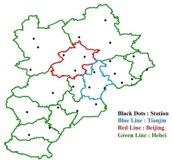
Figure 1.
Study area map.
Because the climate in the Beijing–Tianjin–Hebei region is a warm temperate continental monsoon type, there is little rain in winter and it is rainy in summer. As shown in Figure 2, the distribution of rainfall days in the rainy season (June to September) and the non-rainy season (January to May, October to December) are quite different. If we directly use all the data to build the model, this will cause the model to be unable to better learn the laws of the data, so according to the local seasonal characteristics, we respectively establish the rainfall prediction model based on the rainy-season data (Rainy-Model) and the rainfall prediction model based on the non-rainy-season data (Drier-Model).
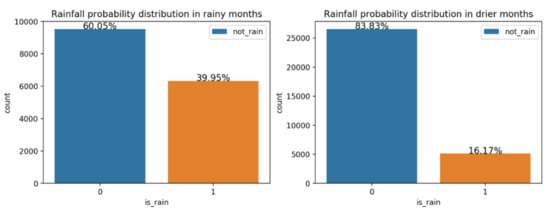
Figure 2.
Rainfall probability distribution.
We predicted the rainfall for each station in the next 30 days. We chose September 2016 as the test set of Rainy-Model, and December 2016 as the test set of Drier-Model. The reason for not using cross-validation to randomly select the test set was to ensure the order of the time-series prediction.
Table 2 and Table 3 describe the division of the data set of the rainy season model and the dry season model, respectively. We selected the data for one consecutive month as the verification set and the test set to ensure that the model could capture the continuity of rainfall.
Table 2.
Rainy-Model’s data set description.
Table 3.
Drier-Model’s data set description.
3. Methodology
3.1. TabNet
The neural network was based on the extension of the perceptron, and deep neural networks (DNNs) can be understood as neural networks with many hidden layers. At present, DNNs have achieved great success in images [18], text [19], and audio [20]. However, for tabular data sets, ensemble tree models are still mainly used. In many data-mining competitions, Xgboost [21] and Lightgbm [22] have been widely used. These rely on the following:
- (1)
- The tree model has a decision manifold [23], which approximates the boundary of the hyperplane. The boundary of the hyperplane can effectively divide the data so that the tree model has an efficient representation of tabular data.
- (2)
- Good interpretability.
- (3)
- Fast training speed.
Secondly, the previously proposed DNN structure is not suitable for tabular data. Traditional DNN based on convolutional layers or multi-layer perceptron (MLP) often have too many parameters for tabular data and lack proper inductive bias, which makes them unable to find the decision manifold for tabular data. The main disadvantage of the decision tree and its variant model is the dependency of feature engineering. A very important reason why deep learning methods can achieve great success in images, natural language, and audio is that deep learning can encode raw data into meaningful representations. End-to-end training based on the backpropagation algorithm can effectively encode tabular data, thereby reducing or even eliminating the need for feature engineering. Not only that, when the data set is larger, the expressive ability of the neural network model may have a better effect.
Figure 3 shows that the TabNet encoder architecture is mainly composed of a feature transformer, an attentive transformer, and feature masking at each decision step. The tabular data includes category data and numeric data. TabNet uses original numerical data and uses trainable embedding [24] to map categorical features to numerical features. Each decision step inputs the same B × D feature matrix; B is the size of the batch size, and D is the dimension of the feature. TabNet’s encoding is based on the processing of multiple decision steps. The characteristics of each decision step are determined by the output of the previous decision step through the Attentive transformer. This outputs the processed feature representation and integrates it into the overall decision-making.
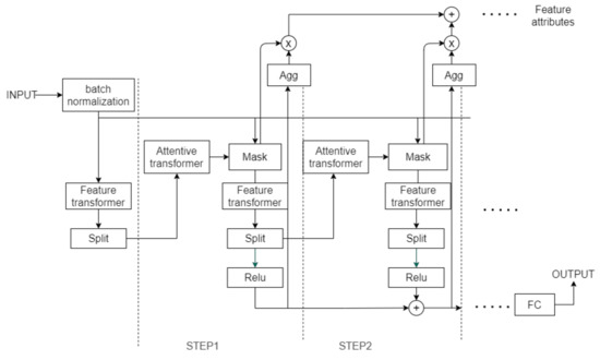
Figure 3.
The encoder of the TabNet architecture.
3.1.1. Feature Selection
Feature selection is realized by the Mask module of each decision step. The Attentive converter of the decision step selects the function to be implemented.
As shown in Figure 4, the Attentive transformer realizes the feature selection of the current decision step by learning a mask. The sequence number in Figure 2 represents the sequence of tensor flow, and the specific meaning is as follows:
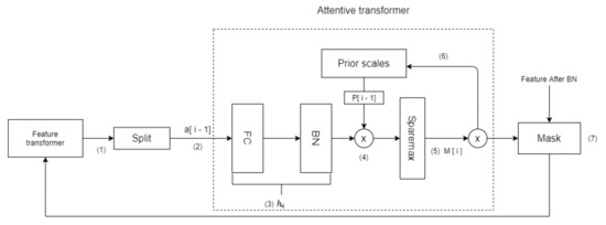
Figure 4.
The topological structure of the Attentive transformer layer.
- (1)
- First, the Feature transformer of the previous decision step outputs the tensor and sends it to the Split module.
- (2)
- The Split module splits the tensor in step 1 and obtains .
- (3)
- passes through the layer, which represents a fully-connected (FC) layer and a BN layer. The role of is to achieve the linear combination of features, thereby extracting higher-dimensional and more abstract features.
- (4)
- The output of the layer is multiplied by the prior scale of the previous decision step. The prior scale represents the use of features in previous decision steps. The more features used in the previous decision step, the smaller the weight in the current decision step.
- (5)
- The is then generated through Sparsemax [25]. Equation (1) represents this process of learning a mask:Sparsemax encourages sparsity by mapping the Euclidean projection onto the probabilistic simplex, make feature selection more sparse. Sparsemax can make , where D represents the dimension of the feature. Sparsemax implements weight distribution for each feature, j, of each sample, b, and makes the sum of the weights of all features of each sample to 1, thus realizing instance-wise [26] feature selection which makes TabNet use the most beneficial features for the model in each decision step. To control the sparsity of the selected features, TabNet uses the sparse regular term:When most of the features of the data set are redundant, the sparsity of feature selection can provide better inductive bias for convergence to a higher accuracy rate.
- (6)
- uses Equation (3) to update :When γ = 1, it means that each feature can only appear in one decision step.
- (7)
- and feature elements are multiplied to realize the feature selection of the current decision step.
- (8)
- The selected features are then inputted into the feature transformer of the current decision step, and a new decision step loop is started.
3.1.2. Feature Processing
The features filtered by Mask are sent to the Feature transformer layer for feature processing. The processed features are divided into two parts by the split module; one part is used for the output of the current decision step, and the other part is used as the input information of the next decision step. The above process is expressed in Equation (4):
The Feature transformer layer is composed of the BN layer, gated linear unit (GLU) layer, and FC layer. The structure is shown in Figure 5.
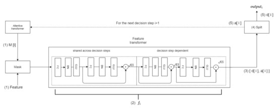
Figure 5.
The topological structure of the Feature transformer layer.
It can be seen that the Feature transformer layer consists of two parts. The parameters of the first half of the layer are shared, which means that they are jointly trained on all steps, while the second half is not shared, and is trained separately on each step. For each step, the input is the same features, so we can use the same layer to do the common part of the feature calculation, and then use different layers to do the feature part of each step. This structure will make the model have robust learning with high capacity. The residual connection is used in the layer, and it is multiplied by to ensure the stability of the network.
3.1.3. TabNet Decoder Architecture
The encoded representation in Figure 6 is the sum vector of the encoder without the FC layer. The encoded representation is used as the input of the decoder. The decoder uses the Feature transformer layer to reconstruct the representation vector into a feature. After the addition of several steps, we output the reconstructed feature.
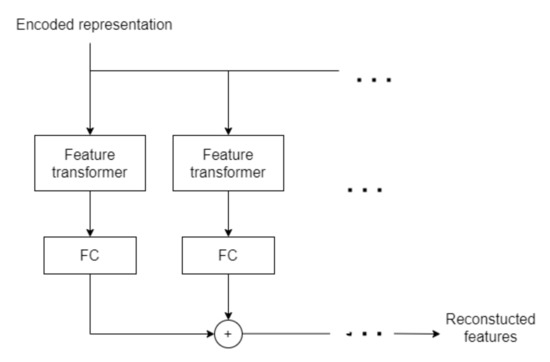
Figure 6.
The topological structure of the decoder.
3.2. Feature Engineering
To make the model better learn the laws of data, we used feature engineering to improve the model. Feature engineering is the process of transforming raw data into features that better represent the underlying problem to the predictive models, resulting in improved model accuracy on hidden data, which usually includes feature selection, feature preprocessing, and feature construction. The feature selection method has been introduced in detail in Section 3.1.1. Section 3.2.1. mainly introduces the feature construction used in this research and Section 3.2.2. mainly introduces the statistical features used in this research.
3.2.1. Feature Construction
To help the model learn the laws of the data better, we used feature construction methods to combine features through different parameters. Feature construction is the manual construction of new features from raw data or new data, it is an important method to increase the model limit.
Precipitable water vapor (PWV) was used to quantify the water vapor content in the troposphere to make the measurement more accurate. PWV refers to the amount of precipitation formed by the condensation of water vapor into rain in the air column of the unit cross-section from the ground to the top of the atmosphere [27]. However, rainfall is affected by complex factors. To improve the accuracy of predicting rainfall, we cannot just use the PWV indicator.
Zenith total delay (ZTD) occurs as the Global Navigation Satellite System (GNSS) signal is affected by the atmospheric refraction when it passes through the troposphere, ZTD includes zenith hydrostatic delay (ZHD) and zenith wet delay (ZWD) [28]. ZHD accounts for approximately 90% of ZTD [29]. ZHD can be calculated by using Equation (5):
where PW is the surface pressure of the station with a unit of °C, ϕ refers to the latitude of the station with a unit of a radian, and H is the geodetic height of the station with a unit of km. Therefore, ZWD can be obtained by extracting ZHD from ZTD, and PWV can be calculated by using Equation (6):
where is the water vapor density, and Π represents the conversion factor:
Π is an empirical parameter, which is approximately 1.48 in the northern hemisphere.
We combined pressure, latitude, and the height of the station features into ZTD features according to Equation (5), and combined data, the height of the station, and ZTD into PWV features according to Equations (6) and (7).
We constructed PWV feature which is a common indicator for satellite observation of rainfall, realized the combination of machine learning and traditional methods, and improved the performance of the model.
3.2.2. Statistical Features
We constructed statistical features to help the model learn the distribution of data. Taking into account that each province and city will have different rainfall due to their geographic factors, we constructed the average and standard deviation of the rainfall for each province and city. Taking into account that in each month, due to its seasonal factors, the rainfall will be different, we constructed the average and standard deviation of the rainfall for each month.
Through the above method, we could obtain the average rainfall of each province and each month, so that the model could capture the change information of regions and months, and then learn the changes of the seasons.
We constructed the relationship between the rainfall and the station. If we directly calculated the average rainfall of each station, which would lead to data leakage, because the model would use future information when training, making the model perform poorly on the test set. To solve this problem, We calculated the average rainfall of each station in the previous 7 days. For example, on the 6th day of the station “Bao_Ding”, we calculated the average rainfall from the 1st to the 5th day of the station “Bao_Ding”.
Through the above methods, we could get the average rainfall of each station in the previous 7 days, so that the model could capture the weekly rainfall information of each station, and then learn the changes in rainfall during the seasons.
3.3. Self-Supervised Pretraining
There are two basic learning paradigms in machine learning—one is supervised learning and the other is unsupervised learning. In a supervised learning model, the algorithm learns based on a labeled data set, and the data set provides answers. The algorithm can use the answers to evaluate their accuracy in training data. In contrast, unsupervised models use unlabeled data, and algorithms need to extract features and laws themselves to understand these data. Self-supervised learning mainly uses a pretext to mine its supervision information from large-scale unsupervised data, and trains the network through this constructed supervision information, so that it can learn valuable representations for downstream tasks.
Self-supervised pretraining can constrain the parameters in an appropriate space, so that the pre-training can be initialized in this space, making the weights non-linear, and the loss function will become more complicated, because it has more topological structure, such as mountains and valleys. The existence of these topologies makes it difficult for parameters to move significant distances. The model with pre-training starts from more favorable regions of feature space.
This study used TabNet for self-supervised pre-training. Different features of the same sample are related, so our self-supervised learning was to first mask some features and then use the encoder-decoder model to predict the masked features. The encoder model trained in this way can effectively characterize the features of the sample, speed up model convergence, and enhance the performance of the model.
4. Model Evaluations
This study used modified Kling–Gupta efficiency (KGE), mean absolute error (MAE), random error (RMSE), and mean absolute percentage error (MAPE) as the evaluation metric.
The KGE was developed by Gupta et al. [30] to provide a diagnostically interesting decomposition of the NSE, which facilitates the analysis of the relative importance of its different components (correlation, bias, and variability) in the context of hydrological modeling [31].
where r is the correlation coefficient between the simulated and observed runoff (dimensionless), β is the bias ratio (dimensionless), γ is the variability ratio (dimensionless), u is the mean runoff in m3/s, and CV is the coefficient of variation (dimensionless). The KGE exhibits its optimum value at unity [30].
The greater the deviation between the predicted value and the true value, the greater the value of MAE, and the worse the performance of the model. RMSE describes the degree of dispersion of data. When the RMSE of model A is smaller than model B, the stability of model A is better. MAPE not only considers the error between the predicted value and the true value, but also considers the ratio between the error and the true value.
5. Results
5.1. Hyperparameter
By setting the parameters of the model, if the MAE of the model does not drop 10 times, the learning rate will be halved to help the model converge and make it easier to obtain the best solution. If the MAE of the model does not drop 30 times, the model will stop early to reduce overfitting.
Table 4 shows the hyperparameter settings of TabNet. N_d, N_a, and N_steps are important parameters that determine the capacity of the model. For most data sets, N_steps ranging from 3 to 10 is a reasonable parameter, and N_d = N_a is a reasonable choice [17]. Reducing N_d, N_a, and N_steps is an effective way to reduce overfitting without significantly reducing the accuracy.
Table 4.
The hyperparameter settings of TabNet.
5.2. The Result of Feature Selection
As shown in Figure 7, the probability of rainfall is determined by many factors, so how to better select features will become an important factor affecting model performance. We use the Instance-wise feature selection method of TabNet to select features.
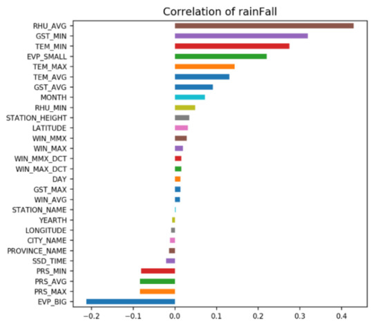
Figure 7.
Correlation of each feature with the probability of rainfall.
Figure 8 shows which features are selected between the first decision step and the third decision step. The brighter color means that at this decision step, the feature is assigned a greater weight. Figure 8 also shows that each decision step will assign a different weight to each feature, which reflects the instance-wise idea.
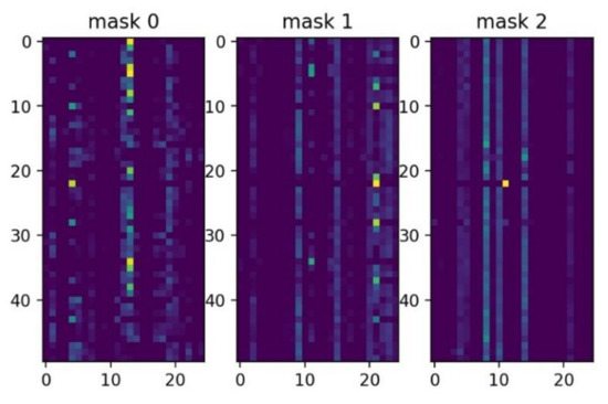
Figure 8.
Feature importance masks M[i] (that indicate which features are selected at ith step).
Figure 9 shows the global importance of each feature. TabNet considers average humidity (RHU_AVG), maximum wind speed (WIN_MAX), average surface temperature (GST_AVG), and daily maximum air pressure (PRS_AVG) to be relatively important. These four features account for 40% of the total feature importance.
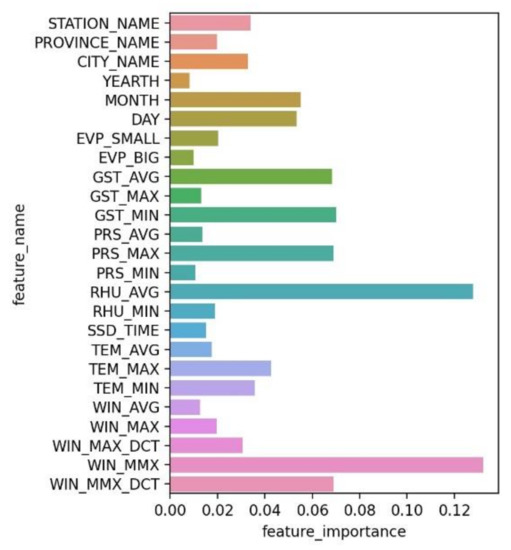
Figure 9.
Global importance of each feature.
5.3. Convergence
The original Rainy-Model converged in 58 epochs and got an MAE of 0.8332 in the test set. Figure 9 shows that the original model had serious oscillation problems in the early stage of training. We used the self-supervised learning of TabNet to help the model speed up convergence and maintain stability. We masked 80% of the features during pretraining.
Figure 10 shows that after the model underwent self-supervised pre-training, the convergence speed became faster. Compared with the original Rainy-Model that completed the convergence at 58 epochs, the new Rainy-Model completed the convergence at 49 epochs. This improvement was more pronounced in larger data sets or more complex tasks. More fast convergence can be highly beneficial particularly in scenarios like continual learning and domain adaptation. The TabNet with Pre-training (TabNet-P) is also more stable and the performance has been improved; the MAE of the test set was 0.7403.
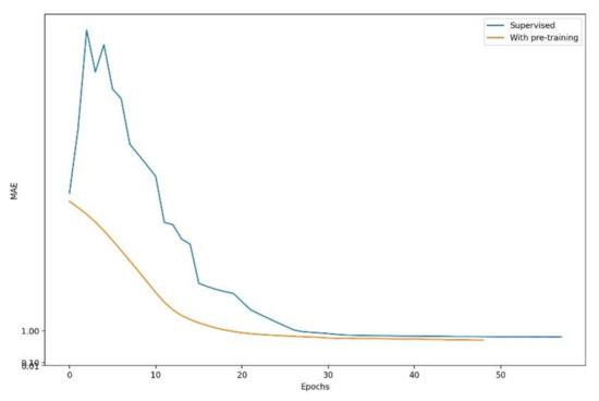
Figure 10.
The model with self-supervised pre-training.
Figure 11 shows the entire experimental process of this study.
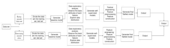
Figure 11.
Experiment process.
6. Discussion
6.1. Extreme Rainfall
When extreme rainfall occurs, the surface temperature and humidity of the day will change drastically. The model learns the changes of these factors to predict the amount of rainfall. The satellite system found that the PWV value will increase sharply before it rains, which proves that the PWV value can well reflect the extreme rainfall. We synthesized the PWV features so that the model can better capture extreme rainfall conditions. Table 5 shows the prediction of extreme rainfall by the model.
Table 5.
Forecast of extreme rainfall. The bolded fields emphasize that extreme rainstorms occurred on that day.
6.2. The Final Model
We used the feature engineering method introduced in Section 3.2.1 and Section 3.2.2 to make TabNet-P better learn data rules to enhance model performance. Table 6 shows part of the output of TabNet with pretraining and feature engineering (TabNet-PF).
Table 6.
Part of the output of TabNet-PF is based on rainy-season data.
Figure 12 shows the learning curve of TabNet-PF generated based on rainy-season data and the learning curve of TabNet-PF generated based on non-rainy-season data. Figure 12 also shows that after pretraining and feature engineering, the performance of TabNet has been significantly improved; the MAE of the test set of TabNet-PF based on rainy-season data is 0.3373, which is better than the MAE of TabNet-P, proving the necessity and rationality of feature engineering.
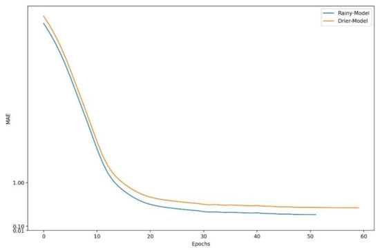
Figure 12.
The learning curve of TabNet-PF.
Table 7 shows the performance differences of the models in different seasons. The performance of the Rainy-Model is better than the Drier-Model, because the data set used by Drier-Model is more imbalanced.
Table 7.
Model performance differences in different seasons.
6.3. Comparative Experiments
This study used BP-NN [32], LSTM [33], Lightgbm as comparative experiments. The BP neural network has good robustness when processing tabular data because its structure is simple; it is only composed of the input layer, hidden layer, and output layer. LSTM solves the vanishing gradient problem caused by the gradual reduction of the gradient backpropagation process, so it is very suitable for handling problems that are highly related to time series. Lightgbm, as an integrated tree model, can fit the hyperplane boundary in tabular data well.
Table 8 shows that TabNet has the best performance when compared with gradient boosted tree and traditional neural network. Table 8 also shows that after pretraining and feature engineering, the difference between the training set MAE and the test set MAE of TabNet was reduced, effectively reducing over-fitting, and proving that the data-mining method we propose has good robustness.
Table 8.
Comparative experiment results.
7. Conclusions
Rainfall is affected by a variety of meteorological factors and is a complex nonlinear system. A rainfall forecast model was proposed based on an improved TabNet neural network by using multiple meteorological parameters. To accelerate model convergence and improve model stability, we optimized the model using self-supervised pre-training. We combined traditional methods with machine learning methods to improve the accuracy of the model and used feature engineering methods to make the model learn the seasonal changes of rainfall. Comparative experiments showed that our proposed model had the best performance. This result proves the reliability of using the model to forecast rainfall. In future research, more data, better parameters, and more reasonable feature engineering methods should be used to increase the robustness of the model.
Author Contributions
methodology, J.Y., T.X., Y.Y., and H.X.; software, T.X.; supervision, J.Y., T.X., Y.Y., and H.X.; writing—original draft, T.X.; writing—review and editing, T.X. All authors have read and agreed to the published version of the manuscript.
Funding
This research was funded by [Water Pollution Control and Treatment Science and Technology Major Project] grant number [2018ZX07111005]. The APC was funded by [Water Pollution Control and Treatment Science and Technology Major Project] and Engineering Research Center of Digital Community of Beijing University of Technology.
Institutional Review Board Statement
Not applicable.
Informed Consent Statement
Not applicable.
Data Availability Statement
The data presented in this study is available on request from the corresponding author.
Acknowledgments
The authors would like to thank the anonymous reviewers for their valuable comments and suggestions, which helped improve this paper greatly.
Conflicts of Interest
The authors declare no conflict of interest.
References
- Jiang, T.; Su, B.; Hartmann, H. Temporal and spatial trends of precipitation and river flow in the Yangtze River Basin, 1961–2000. Geomorphology 2007, 85, 143–154. [Google Scholar] [CrossRef]
- Xingchuang, X.U.; Xuezhen, Z.; Erfu, D.; Wei, S. Research of trend variability of precipitation intensity and their contribution to precipitation in China from 1961 to 2010. Geogr. Res. 2014, 33, 1335–1347. [Google Scholar]
- Pranatha, M.D.A.; Pramaita, N.; Sudarma, M.; Widyantara, I.M.O. Filtering Outlier Data Using Box Whisker Plot Method for Fuzzy Time Series Rainfall Forecasting. In Proceedings of the 2018 4th International Conference on Wireless and Telematics (ICWT), Bali, Indonesia, 12–13 July 2018. [Google Scholar]
- Maheswaran, R.; Khosa, R. A Wavelet-Based Second Order Nonlinear Model for Forecasting Monthly Rainfall. Water Resour. Manag. 2014, 28, 5411–5431. [Google Scholar] [CrossRef]
- Qiu, J.; Shen, Z.; Wei, G.; Wang, G.; Lv, G. A systematic assessment of watershed-scale nonpoint source pollution during rainfall-runoff events in the Miyun Reservoir watershed. Environ. Sci. Eur. 2018, 25, 6514. [Google Scholar] [CrossRef] [PubMed]
- Chau, K.W.; Wu, C.L. A hybrid model coupled with singular spectrum analysis for daily rainfall prediction. J. Hydroinform. 2010, 12, 458–473. [Google Scholar] [CrossRef]
- Zhang, L.; Dai, A.; Hove, T.V.; Baelen, J.V. A near-global, 2-hourly data set of atmospheric precipitable water from ground-based GPS measurements. J. Geophys. Res. Atmos. 2007, 112. [Google Scholar] [CrossRef]
- He, C.; Wu, S.; Wang, X.; Hu, A.; Wang, Q.; Zhang, K. A new voxel-based model for the determination of atmospheric weighted mean temperature in GPS atmospheric sounding. Atmos. Meas. Tech. 2017, 10, 2045–2060. [Google Scholar] [CrossRef]
- Benevides, P.; Catalao, J.; Miranda, P. On the inclusion of GPS precipitable water vapour in the nowcasting of rainfall. Nat. Hazards Earth Syst. Sci. 2015, 3, 3861–3895. [Google Scholar]
- Yin, J.; Guo, S.; Gu, L.; Zeng, Z.; Xu, C.Y. Blending multi-satellite, atmospheric reanalysis and gauge precipitation products to facilitate hydrological modelling. J. Hydrol. 2020, 593, 125878. [Google Scholar] [CrossRef]
- Zhou, Y.; Qin, N.; Tang, Q.; Shi, H.; Gao, L. Assimilation of Multi-Source Precipitation Data over Southeast China Using a Nonparametric Framework. Remote Sens. 2021, 13, 1057. [Google Scholar] [CrossRef]
- Bhuiyan, A.E.; Yang, F.; Biswas, N.K.; Rahat, S.H.; Neelam, T.J. Machine Learning-Based Error Modeling to Improve GPM IMERG Precipitation Product over the Brahmaputra River Basin. Forecasting 2020, 2, 248–266. [Google Scholar] [CrossRef]
- Derin, Y.; Bhuiyan, M.; Anagnostou, E.; Kalogiros, J.; Anagnostou, M.N. Modeling Level 2 Passive Microwave Precipitation Retrieval Error Over Complex Terrain Using a Nonparametric Statistical Technique. IEEE 2020. [Google Scholar] [CrossRef]
- Xiang, B.; Zeng, C.; Dong, X.; Wang, J. The Application of a Decision Tree and Stochastic Forest Model in Summer Precipitation Prediction in Chongqing. Atmosphere 2020, 11, 508. [Google Scholar] [CrossRef]
- Lee, Y.-M.; Ko, C.-M.; Shin, S.-C.; Kim, B.-S. The Development of a Rainfall Correction Technique based on Machine Learning for Hydrological Applications. J. Environ. Sci. Int. 2019, 28, 125–135. [Google Scholar] [CrossRef]
- Zhang, L.; Li, X.; Zheng, D.; Zhang, K.; Ge, Y. Merging multiple satellite-based precipitation products and gauge observations using a novel double machine learning approach. J. Hydrol. 2021, 594, 125969. [Google Scholar] [CrossRef]
- Arik, S.O.; Pfister, T. TabNet: Attentive Interpretable Tabular Learning. arXiv 2019, arXiv:1908.07442. [Google Scholar]
- He, K.; Zhang, X.; Ren, S.; Sun, J. Deep Residual Learning for Image Recognition. arXiv 2015, arXiv:1512.03385. [Google Scholar]
- Conneau, A.; Schwenk, H.; Barrault, L.; Lecun, Y. Very Deep Convolutional Networks for Text Classification. arXiv 2016, arXiv:1606.01781. [Google Scholar]
- Amodei, D.; Anubhai, R.; Battenberg, E.; Case, C.; Casper, J.; Catanzaro, B.; Chen, J.; Chrzanowski, M.; Coates, A.; Diamos, G.; et al. Deep Speech 2: End-to-End Speech Recognition in English and Mandarin. arXiv 2015, arXiv:1512.02595. [Google Scholar]
- Chen, T.Q.; Guestrin, C. XGBoost: A Scalable Tree Boosting System; Association for Computing Machinery: New York, NY, USA, 2016; pp. 785–794. [Google Scholar]
- Ke, G.; Meng, Q.; Finley, T.; Wang, T.; Chen, W.; Ma, W.; Ye, Q.; Liu, T.-Y. LightGBM: A Highly Efficient Gradient Boosting Decision Tree. In Proceedings of the 31st Conference on Neural Information Processing Systems (NIPS 2017), Long Beach, CA, USA, 4–9 December 2018. [Google Scholar]
- Polzlbauer, G.; Lidy, T.; Rauber, A. Decision Manifolds—A Supervised Learning Algorithm Based on Self-Organization. IEEE Trans. Neural Netw. 2008, 19, 1518–1530. [Google Scholar] [CrossRef]
- Grbovic, M.; Cheng, H.B. Real-Time Personalization using Embeddings for Search Ranking at Airbnb; Association for Computing Machinery: New York, NY, USA, 2018; pp. 311–320. [Google Scholar]
- Martins, A.F.T.; Fernandez Astudillo, R. From Softmax to Sparsemax: A Sparse Model of Attention and Multi-Label Classification. arXiv 2016, arXiv:1602.02068. [Google Scholar]
- Yoon, J.; Jordon, J.; van der Schaar, M. INVASE: Instance-Wise Variable Selection using Neural Networks. In Proceedings of the Seventh International Conference on Learning Representations (ICLR), New Orleans, LA, USA, 6–9 May 2019. [Google Scholar]
- Shilpa, M.; Hui, L.Y.; Song, M.Y.; Feng, Y.; Teong, O.J. GPS-Derived PWV for Rainfall Nowcasting in Tropical Region. IEEE Trans. Geosci. Remote Sens. 2018, 56, 4835–4844. [Google Scholar]
- Li, P.; Wang, X.; Chen, Y.; Lai, S. Use of GPS Signal Delay for Real-time Atmospheric Water Vapour Estimation and Rainfall Nowcast in Hong Kong. In Proceedings of the The First International Symposium on Cloud-Prone and Rainy Areas Remote Sensing, Chinese University of Hong Kong, Hong Kong, 6–8 October 2005; pp. 6–8. [Google Scholar]
- Saastamoinen, J.H. Atmospheric Correction for the Troposphere and the Stratosphere in Radio Ranging Satellites. In The Use of Artificial Satellites for Geodesy; American Geophysical Union: Washington, DC, USA, 1972; Volume 15. [Google Scholar]
- Gupta, H.V.; Kling, H.; Yilmaz, K.K.; Martinez, G.F. Decomposition of the mean squared error and NSE performance criteria: Implications for improving hydrological modelling. J. Hydrol. 2009, 377, 80–91. [Google Scholar] [CrossRef]
- Kling, H.; Fuchs, M.; Paulin, M. Runoff conditions in the upper Danube basin under an ensemble of climate change scenarios. J. Hydrol. 2012, 424–425, 264–277. [Google Scholar] [CrossRef]
- Liu, X.S.; Deng, Z.; Wang, T.L. Real estate appraisal system based on GIS and BP neural network. Trans. Nonferrous Met. Soc. China 2011, 21, s626–s630. [Google Scholar] [CrossRef]
- Hochreiter, S.; Schmidhuber, J. Long Short-Term Memory. Neural Comput. 1997, 9, 1735–1780. [Google Scholar] [CrossRef] [PubMed]


Publisher’s Note: MDPI stays neutral with regard to jurisdictional claims in published maps and institutional affiliations. |
© 2021 by the authors. Licensee MDPI, Basel, Switzerland. This article is an open access article distributed under the terms and conditions of the Creative Commons Attribution (CC BY) license (https://creativecommons.org/licenses/by/4.0/).