Analytical Models of Velocity, Reynolds Stress and Turbulence Intensity in Ice-Covered Channels

Abstract

Ice cover in an open channel can influence the flow structure, such as the flow velocity, Reynolds stress and turbulence intensity. This study analyzes the vertical distributions of velocity, Reynolds stress and turbulence intensity in fully and partially ice-covered channels by theoretical methods and laboratory experiments. According to the experimental data, the vertical profile of longitudinal velocities follows an approximately symmetry form. Different from the open channel flow, the maximum value of longitudinal velocity occurs near the middle of the water depth, which is close to the channel bed with a smoother boundary roughness compared to the ice cover. The measured Reynolds stress has a linear distribution along the vertical axis, and the vertical distribution of measured turbulence intensity follows an exponential law. Theoretically, a two-power-law function is presented to obtain the analytical formula of the longitudinal velocity. In addition, the vertical profile of Reynolds stress is obtained by the simplified momentum equation and the vertical profile of turbulence intensity is investigated by an improved exponential model. The predicted data from the analytical models agree well with the experimental ones, thereby confirming that the analytical models are feasible to predict the vertical distribution of velocity, Reynolds stress and turbulence intensity in ice-covered channels. The proposed models can offer an important theoretical reference for future study about the sediment transport and contaminant dispersion in ice-covered channels.

1. Introduction

Most rivers at high altitude in cold northern regions always freeze in the winter and form ice sheets. The ice sheet in some Canadian rivers is at least 0.6 m thick and lasts for at least 4 months [1]. The wetted perimeter of the cross section and flow resistance in ice-covered flows increases with the presence of the ice sheet, which significantly affects the hydraulic characteristics of river and topographical features and greatly change the flow velocity distribution, flow transport capacity and sediment transport rate [2,3,4,5,6,7,8,9,10,11]. Therefore, it is necessary to study the ice-covered flows.

Unlike the open channel flow, flows in the ice-covered channel have asymmetric forms. The presence of the ice sheet makes the maximum streamwise velocity appear at the inner center of the flow, and the location of the maximum velocity is generally considered the division point in the asymmetrically distributed flow [12,13]. The asymmetric distribution mainly depends on the roughness of the ice sheet and the riverbed. The division point of the velocity tends to be away from the rougher surface [14]. Previous studies have shown that the main effects of the ice sheets on alluvial channels can be summarized as: they increase the water level (compared to open channels at the same flow rate), reduce the average flow velocity, increase the channel drag force and reduce the bed sediment transport rate [15].

Previous investigations on the flow characteristics of ice-covered flows are mainly obtained through experiments [16,17,18]. Many laboratory experimental data and field observations show that the vertical distribution of streamwise velocity forms a double-layer, which is characterized by the plane of maximum velocity. Shen and Harden (1978) [19] and Lau and Krishnappan (1981) [20] applied this double-layer theory in the ice-covered flows. They divided the ice-covered flows into two separate layers: upper ice layer and lower channel bed. Parthasarathy and Muste (1994) [13] found that the zero shear stress plane in the ice-covered flows was inconsistent with the maximum velocity plane. Chen et al. (2015) [21] proposed that the horizontal plane of zero shear stress should be determined as the dividing plane of sublayers and modified the double-layer assumption.

Some researchers have studied the vertical profiles of the longitudinal velocity by numerical simulation methods and proposed two-dimensional and three-dimensional models [22,23], which may require sensitive hydraulic parameters. However, these hydraulic parameters do not have explicit expressions to be calculated, and they have uncertainty that cannot be ignored. Except the numerical methods, previous researchers also attempted to obtain the vertical distribution of streamwise velocity by theoretical methods [24,25]. Uzuner (1975) [26] separated the ice-covered flow into two layers based on the position of the maximum velocity and assumed that the velocity distributions in the upper ice layer and lower bed layer were consistent with the logarithmic distribution law, and Manning formula could be independently applied to each layer. In addition, a two-power-law function was adopted to calculate the vertical distribution of the longitudinal velocity. Teal et al. (1994) [27] reported a reasonable fit of streamwise velocity data to the two-power-law function. Compared to the two-power-law function, the logarithmic law appears to overestimate velocities near the location of maximum velocity. The two-power-law function is a reasonable extension of the power-law expression that is used to describe velocity profiles of open channel flow. The advantage for the two-power-law function is that it describes the entire flow with a single continuous curve. Hence, the two-power-law function deserves further study.

The objective of this study is to obtain the vertical profiles of longitudinal velocity, Reynolds stress and turbulence intensity in ice-covered channels. Hence, this study focuses on (1) adopting a two-power-law function to calculate the vertical profile of the longitudinal velocity, (2) simplifying the time-averaged momentum equation to analyze the vertical distributions of Reynolds stress, (3) improving the exponential model to calculate the turbulence intensity and (4) employing experimental data to validate the theoretical models and giving detail discussion on the coefficients in the theoretical models.

2. Material and Methods

Since the free water surface is covered with ice, the open channel flow changes to a closed conduit flow but retains the flow characteristics of the open channel flow. The vertical distribution of longitudinal velocity significantly changes in the open channel flow with ice-cover, which reflects that the plane of maximum longitudinal velocity shifts from the free water surface to the inner water (see Figure 1). Here, we used a Cartesian coordinate system with the $x$ axis in the main flow direction and $z$ axis in the water depth direction. Corresponding to the $x$ and $z$ axes, $u$ and $w$ are the longitudinal and vertical velocities, respectively.

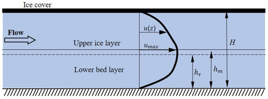
Figure 1. Schematic profile of the longitudinal velocity in an iced-covered open channel.

2.1. Vertical Distribution of Longitudinal Velocity

The presence of the ice cover causes the increase of the wetted perimeter, which increases the composite flow resistance. Owing to the different roughness of ice cover and channel bed, the velocity profile is vertically asymmetric (see Figure 1). In Figure 1, the vertical flow structure can be divided into two independent layers at the plane of maximum velocity, i.e., the upper ice layer and lower bed layer. The flow in the upper ice layer is mainly affected by the ice cover, and the lower flow is primarily affected by the channel bed. The vertical location of the maximum velocity is determined by the roughness of the ice cover and channel bed, i.e., the maximum velocity will not occur at the free water surface but near the middle of the water depth.

Tsai and Ettema (1994) [28] adopted a power-law function to predict the velocity profile in the open channel flow. For the ice-covered flow, a two-power-law function was used to obtain the vertical profile of the longitudinal velocity [27]. The first advantage of the two-power-law function is that it describes the flow just using a single continuous curve. The second is that the analytical solution of velocity is adjustable in accordance with the roughness change of channel bed and ice cover. The two-power-law is shown as

$$u=K_0{\left(\frac{z}{H}\right)}^{1/m_b}{\left(1-\frac{z}{H}\right)}^{1/m_i}$$

(1)

where $z$ is the vertical axis with $z$ = 0 at the channel bed; $H$ is the water depth; $K_0$ is the flow parameter based on a given flow discharge per unit flow width and $m_b$ and $m_i$ are the parameters corresponding to the boundary roughness of the channel bed and ice cover. When parameter $m_i$ approaches infinity, the velocity profile becomes equivalent to a single power law expression, which indicates that the ice cover disappears.

The velocity gradient obtained from Equation (1) is

$$\frac{du}{dz}=\frac{K_0}{H}\left[\frac{1}{m_b}{\left(\frac{z}{H}\right)}^{\frac{1}{m_b}-1}{\left(1-\frac{z}{H}\right)}^{1/m_i}-\frac{1}{m_i}{\left(\frac{z}{H}\right)}^{\frac{1}{m_b}}{\left(1-\frac{z}{H}\right)}^{\frac{1}{m_i}-1}\right]$$

(2)

By setting the velocity gradient $\frac{\partial u}{\partial z}$ to zero, we deduced the position of the maximum velocity as

$${\left(\frac{z}{H}\right)}_{u_{max}}=\frac{h_m}{H}=\frac{m_i}{m_i+m_b}$$

(3)

where $u_{max}$ is the maximum longitudinal velocity and $h_m$ is the height of the maximum velocity from the channel bed.

2.2. Vertical Distribution of Reynolds Stress

To predict the vertical distribution of Reynolds stress in ice-covered channels for a steady uniform flow, the time-averaged momentum equation in the longitudinal direction can be simplified to

$$-\overline{u^{\prime }{w}^{\prime }}+\nu \frac{du}{dz}+\frac{u_{\ast i}^{2}z}{H}=u_{\ast b}^2\left(1-\frac{z}{H}\right)$$

(4)

where $u^{\prime }$ and $w^{\prime }$ are turbulent fluctuations of the longitudinal and vertical velocities, $-\overline{u^{\prime }{w}^{\prime }}$ is Reynolds stress; $\nu$ is the flow kinematic viscosity; $u_{\ast i}$ is the shear velocity at the ice cover and $u_{\ast b}$ is the shear velocity at the channel bed.

Since the viscosity shear stress in the flow is much smaller than the Reynolds stress, the viscosity shear stress can be neglected in Equation (4) [29,30]. Then, there is a linear relationship between the shear stress $\left(\tau \right)$ and the vertical axis $\left(z\right)$. Equation (4) has another form and is shown as

$$\tau \left(z\right)={\tau }_b-\left({\tau }_b-{\tau }_i\right)\frac{z}{H}$$

(5)

where $\tau \left(z\right)$ is the shear stress at distance $z$; ${\tau }_b$ and ${\tau }_i$ are the Reynolds stresses at the channel bed and ice cover; $z$ is the vertical distance from the channel bed and $H$ is the water depth.

Following the method of Rowinski and Kubrak (2002) [31], who combine the eddy viscosity and flow conditions by a mixing length concept, the shear stress can be given as

$$\tau \left(z\right)=\rho l^2\frac{\partial u}{\partial z}\left|\frac{\partial u}{\partial z}\right|$$

(6)

where $\rho$ is the flow density and $l$ is the proposed mixing length. Chen et al. (2015) [21] demonstrate that the mixing length theory can be applied at a certain distance from the fixed boundaries. Two mixing lengths, $l_b$ and $l_i$, are proposed corresponding to the two fixed boundaries. The first one is the mixing length of channel bed and the second one is the mixing length of the ice cover. Hence, the linear relationships of two mixing lengths are approximately written as

$$\{\begin{array}{c}{l}_b=\kappa z, 0\le z\le {\delta }_b\\ l_i=\kappa \left(H-z\right), H-{\delta }_i\le z\le H\end{array}$$

(7)

where ${\delta }_b$ and ${\delta }_i$ are the distances from the channel bed and ice cover, where the mixing length theory is valid. $\kappa$ = 0.41 is the von Karman constant.

By substituting Equation (7) into Equation (6), we updated the expression of shear stress as

$$\{\begin{array}{c}\tau \left(z\right)=\rho {\kappa }^2{z}^2\frac{\partial u}{\partial z}\left|\frac{\partial u}{\partial z}\right|, 0\le z\le {\delta }_b\\ \tau \left(z\right)=\rho {\kappa }^2{\left(H-z\right)}^2\frac{\partial u}{\partial z}\left|\frac{\partial u}{\partial z}\right|, H-{\delta }_i\le z\le H\end{array}$$

(8)

The gradient of shear stress from Equation (8) is

$$\{\begin{array}{c}\frac{\partial \tau }{\partial z}=2\rho {\kappa }^2{z}^2\frac{\partial u}{\partial z}\left(\frac{1}{z}\frac{\partial u}{\partial z}+\frac{{\partial }^{2}u}{\partial z^2}\right), 0\le z\le {\delta }_b\\ \frac{\partial \tau }{\partial z}=2\rho {\kappa }^2{\left(H-z\right)}^2\frac{\partial u}{\partial z}\left(\frac{1}{\left(H-z\right)}\frac{\partial u}{\partial z}-\frac{{\partial }^{2}u}{\partial z^2}\right), H-{\delta }_i\le z\le H\end{array}$$

(9)

By substituting the velocity gradient (Equation (2)) into the Reynolds stress gradient (Equation (9)) and letting $\frac{\partial \tau }{\partial z}=0$, we obtained the two maximum Reynolds stresses, ${\tau }_{bmax}$ and ${\tau }_{imax}$, near the channel bed and ice cover, respectively, which are presented as

$$\{\begin{array}{c}{\tau }_{bmax}=\rho {\kappa }^2{z}_{bmax}{}^2\frac{\partial u}{\partial z_{bmax}}\left|\frac{\partial u}{\partial z_{bmax}}\right|, 0\le z\le {\delta }_b\\ {\tau }_{imax}=\rho {\kappa }^2{\left(H-z_{imax}\right)}^2\frac{\partial u}{\partial z_{imax}}\left|\frac{\partial u}{\partial z_{imax}}\right|, H-{\delta }_i\le z\le H\end{array}$$

(10)

where $z_{bmax}$ and $z_{imax}$ denote the positions where the corresponding maximum shear stresses ${\tau }_{bmax}$ and ${\tau }_{imax}$ occurred, and they can be calculated as

$$\{\begin{array}{c}{z}_{\mathit{bmax}}=\frac{-A_b-\sqrt{A_b^2-4B_b{C}_b}}{2B_b}H\\ z_{\mathit{imax}}=\frac{-A_i-\sqrt{A_i^2-4B_i{C}_i}}{2B_i}H\end{array}$$

(11)

where $A_b$, $B_b$, $C_b$, $A_i$, $B_i$, and $C_i$ are the constants relevant to the roughness of the channel bed and ice cover. Their expressions are

$$\{\begin{array}{c}\{\begin{array}{c}{A}_b=-m_b-2\frac{m_i}{m_b}-2\\ B_b=\left(m_b+m_i\right)\left(\frac{1}{m_b}+\frac{1}{m_i}\right)\\ C_b=\frac{m_i}{m_b}\end{array}\\ \{\begin{array}{c}{A}_i=-m_i+2\frac{m_i}{m_b}+2\\ B_i=-\left(m_b+m_i\right)\left(\frac{1}{m_b}+\frac{1}{m_i}\right)\\ C_i=m_i-\frac{m_i}{m_b}\end{array}\end{array}$$

(12)

The shear stresses at the fixed boundaries, i.e., the channel bed and ice cover, can be considered the maximum shear stresses in the lower bed layer and upper ice layer. Hence, the linear relationship (Equation (5)) between shear stress and vertical position can be rewritten as

$$\tau \left(z\right)={\tau }_{bmax}-\left({\tau }_{bmax}-{\tau }_{imax}\right)\frac{z}{H}$$

(13)

2.3. Vertical Distribution of Turbulence Intensity

The flow turbulence characteristics can be presented by the turbulence intensity, which can be calculated by the root mean square of the fluctuating longitudinal velocity, i.e., $u_{rms}=\sqrt{{\left(u^{\prime }\right)}^2}$. In the open channel flow, the term $u_{rms}$ reaches its maximum value near the channel bed and it has a linear relationship with the vertical distance. Nezu and Rodi (1986) [32] established an exponential model to describe the vertical distribution of the turbulence intensity. However, in the ice-covered channel flow, it first decreases from the channel bed and reaches its minimum value near the middle flow depth, after which it gradually increases towards to the ice cover. For the profile of the turbulence intensity in the ice-covered channel, we adopted the division scheme to investigate the profile of the turbulence intensity. Based on the location of zero shear stress, its profile is separated into two regions. Then, the exponential model can be applied in each region as follows

$$\{\begin{array}{c}\frac{u_{rms}}{u_{\ast b}}=D_b{e}^{-E_{b}z/h_{\tau }},0<z<h_{\tau }\\ \frac{u_{rms}}{u_{\ast i}}=D_i{e}^{-E_{i}z/h_{\tau }},h_{\tau }<z<H\end{array}$$

(14)

where $D_b$, $E_b$, $D_i$ and $E_i$ are constant parameters.

3. Experimental Verification

Experiments were performed in a rectangular glass flume with a total length of 20 m, a width of 1 m and a depth of 0.5 m in the State Key Laboratory of Water Resources and Hydropower Engineering Science in Wuhan University to investigate the longitudinal velocity profile in the ice-covered flow (Figure 2). The flow is circulated by a pump system and adjusted to be steady by a tailgate at the end of the flume. A plastic foam board was used to simulate the ice with the length of 15 m and a width of 1 m [33].

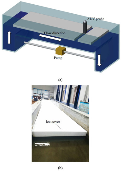
Figure 2. (a) Schematic of the experimental flume, the dark blue denoting the flow in the flume and (b) images of the experimental site.

The rectangular coordinates are as follows: x is the main flow direction with x = 0 at the beginning of the ice cover; y is the lateral direction with y = 0 at the sidewall and z is the vertical direction counting from the channel bed. The velocity was measured at the cross section with x = 9 m, which is sufficiently far from the ice cover entry to form a fully developed flow. In the measured cross section, 14 measured lines are arranged, where the measured points are also arranged with a uniform vertical distance 1 cm. The detail layout is shown in Figure 3.

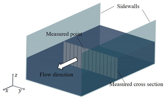
Figure 3. Layout of the measured cross section, lines and points.

A 3D acoustic Doppler velocimeter (ADV) with a precision of ±0.25 cm/s was adopted to measure the instantaneous velocity. The maximum sampling frequency was 50 Hz, and the sampling time for every measured point was 120 s, which resulted in 6000 velocity data for each point. Five experimental conditions were considered here, and the variables among these five cases were the cover conditions and water depth H, which changes from 15 to 20 cm. The details of the experimental parameters are listed in Table 1.

Table 1. Basic details of the characteristic parameters. $B$ is the width of the flume, $H$ is the water depth, $S$ is the bed slope and $Re$ is the Reynolds number.

Cases	Cover Condition	$\mathit{B}$ (m)	$\mathit{H}$ (m)	$\mathit{S}$	$\mathit{R}\mathit{e}$
1	Full ice cover	1	0.15	0.001	25590
2	Full ice cover	1	0.185	0.001	33725
3	Symmetrical shore cover	1	0.16	0.001	32480
4	Symmetrical shore cover	1	0.20	0.001	49160
5	Asymmetrical shore cover	1	0.16	0.001	31888

4. Model Parameters

To predict the profiles of velocity, Reynolds stress and turbulence intensity in the ice-covered flow, the model parameters, i.e., $m_b$ and $m_i$, $n_b$ and $n_i$, $K_0$, etc., should be given first.

4.1. $m_b$ and $m_i$

In the single-power law for the free surface flow, exponent $m$ is affected by Darcy–Weisbach resistance coefficient $f,$ i.e., $m=\kappa {\left(\frac{8}{f}\right)}^{0.5}$ [30]. For the two-power expression, exponents $m_b$ and $m_i$ can also be related to Darcy–Weisbach resistance coefficients of channel bed $f_b$ and ice cover $f_i$. Specifically, the value of one exponent $m$ can be related to the resistance coefficient of one fixed boundary. Hence, exponents $m_b$ and $m_i$ can be expressed as

$$\{\begin{array}{c}{m}_b=\kappa {\left(\frac{8}{f_b}\right)}^{0.5}\\ m_i=\kappa {\left(\frac{8}{f_i}\right)}^{0.5}\end{array}$$

(15)

The resistance coefficients can be calculated as [34]

$$\{\begin{array}{c}{f}_b=\frac{8n_b^{2}g}{R_b^{1/3}}\\ f_i=\frac{8n_i^{2}g}{R_i^{1/3}}\end{array}$$

(16)

where $n$ denotes Manning’s roughness coefficients; $R$ indicates the hydraulic radiuses and the subscript $b$ and $i$ in them represent the channel bed and ice cover. $g$ is the gravity acceleration. Here, the ratio of channel width to water depth was approximately greater than 5, which indicates that the flow could be considered a shallow flow. Hence, the hydraulic radius of each sublayer could be simplified as the corresponding sublayer depth, i.e., $R_b=h_b$ and $R_i=h_i$. The flow depths of the lower bed layer and upper ice layer have been defined from the location of the maximum velocity and are represented by $h_m$ and $H-h_m$. Hence, we easily obtained

$$\{\begin{array}{c}{h}_m=h_b\\ H-h_m=h_i\end{array}$$

(17)

Substituting Equation (16) into Equation (15), we obtained

$$\{\begin{array}{c}{m}_b=\kappa {\left(\frac{R_b^{1/3}}{n_b^{2}g}\right)}^{0.5}\\ m_i=\kappa {\left(\frac{R_i^{1/3}}{n_i^{2}g}\right)}^{0.5}\end{array}$$

(18)

Then, we substituted Equations (17) and (18) into Equation (3) ($\frac{h_m}{H}=\frac{m_i}{m_i+m_b}$) and obtained

$$h_b=\frac{H{n}_b{\left(H-h_b\right)}^{1/6}}{n_b{\left(H-h_b\right)}^{1/6}+n_i{h}_b{}^{1/6}}$$

(19)

Once Manning’s coefficients $n_b$ and $n_i$ are known, the depth of the lower bed layer ($h_b$) is iteratively solved. Then, exponents $m_b$ and $m_i$ were calculated by Equation (18).

4.2. $n_b$ and $n_i$

The basic calculation model of Darcy–Weisbach friction coefficient $f$ is

$$f=\frac{8u_{\ast }^2}{U^2}$$

(20)

where $U\left(=Q/BH\right)$ is the averaged velocity in a cross section. Substituting Equation (16) into Equation (20), we obtained

$$n=\frac{u_{\ast }}{U\sqrt{g}}{R}^{1/6}$$

(21)

For the ice-covered flow, the flow is divided as two layers, and two depth-averaged velocities, $U_b$ and $U_i$, are averaged from the channel bed and ice cover to the position of the maximum velocity. Hence, Manning’s coefficient in each sublayer can be expressed as

$$\{\begin{array}{c}{n}_b=\frac{u_{\ast b}}{U_b\sqrt{g}}{h}_b^{1/6}\\ n_i=\frac{u_{\ast i}}{U_i\sqrt{g}}{h}_i^{1/6}\end{array}$$

(22)

These two Manning’s parameters can be determined by the measured velocity profile.

For the fully developed asymmetric flow, the method of logarithmic law can be adopted to predict the vertical distribution of the longitudinal velocity. However, because the velocity gradient of the maximum velocity is discontinuous, the method of logarithmic law may not be completely feasible for the entire water depth. For the ice-covered flow, the method of logarithmic law can be applied in each sublayer, i.e., the lower bed layer and upper ice layer. Bonakdari et al. (2008) [35] further demonstrate that the turbulent boundary layer consists of the inner region near the sidewall and outer region far from the sidewall and propose that the flow velocity inside the inner region can better satisfy the distribution form of the logarithmic law. In this study, we define that the inner region inside the lower bed layer starts from the channel bed ($z$ = 0) to 0.2$H$, and the inner region inside the upper ice layer is from 0.8$H$ to the ice cover ($H$). Therefore, we used the following logarithmic law to describe the velocity profile in the two inner regions [36]

$$\{\begin{array}{c}\frac{U_b}{u_{\ast b}}=\frac{1}{\kappa }ln\left(30\frac{z}{k_{sb}}\right)\\ \frac{U_i}{u_{\ast i}}=\frac{1}{\kappa }ln\left(30\frac{z}{k_{si}}\right)\end{array}$$

(23)

where $k_{sb}$ and $k_{si}$ are the roughness heights of the turbulence boundary in the lower bed layer and upper ice layer. The logarithmic law can be simplified to

$$\{\begin{array}{c}{U}_b=a_{b}ln\left(z\right)+F_b\\ U_i=a_{i}ln\left(z\right)+F_i\end{array}$$

(24)

where $a_b=u_{\ast b}/\kappa$, $a_i=u_{\ast i}/\kappa$, $F_b=a_b\left(ln\frac{30}{k_{sb}}\right)$ and $F_i=a_i\left(ln\frac{30}{k_{si}}\right)$. These parameters can be obtained by regression analysis based on the measured longitudinal velocity data; then, shear velocities $u_{\ast b}$ and $u_{\ast i}$ and roughness heights $k_{sb}$ and $k_{si}$ can be obtained.

4.3. $K_0$

According to the previous work [28,37], $K_0$ is the flow model parameter for a known flow rate per unit flow width and is

$$K_0=U/K_1$$

(25)

where $K_1$ is the normalized depth-averaged velocities for total flow and is calculated by

$$K_1={{\displaystyle \int }}_0^1{\left(\frac{z}{H}\right)}^{1/m_b}{\left(1-\frac{z}{H}\right)}^{1/m_i}d\left(z/H\right)$$

(26)

5. Results and Discussion

5.1. Model Verification

With the above model parameters, the theoretical model can be applied to the experimental data. Figure 4 compares the predicted velocity from the model with the measured ones. Both profiles followed the assumed one, where the maximum velocity occurs near the middle of the water depth, and the minimum velocity appears near the fixed boundaries. The analytical results were consistent with the experimental velocities, so the proposed model and corresponding parameters are reasonable and reliable to be used to predict the velocity profile in the straight open channel flow covered by the ice cover.

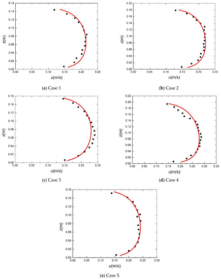
Figure 4. Comparison of the measured and analytical velocities. Black squares denote the measured data and red lines denote the analytical ones.

Figure 5 presents the profiles of measured Reynolds stress and analytical Reynolds stress for all experimental cases. The Reynolds stress in the longitudinal direction demonstrates a linear distribution along the water depth. Zero shear stress occurred at the location of $h_{\tau }$ near the middle of the water depth, after which the absolute value of Reynolds stress gradually increased and reached each peak near the fixed boundaries. The measured and predicted data in Figure 5 were basically consistent and had identical trends, which indicates that our proposed model for Reynolds stresses was feasible.

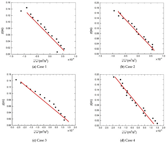
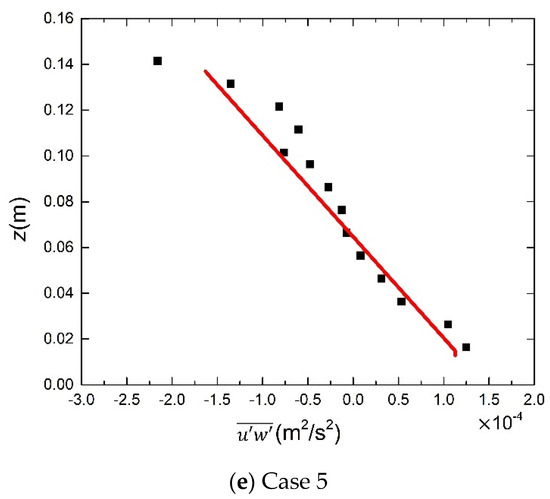
Figure 5. Comparison of the measured and analytical Reynolds stresses. Black squares denote the measured data and red lines denote the analytical ones.

Figure 6 shows the results of the turbulence intensity from the experiments and analytical model. The turbulence intensity reached its minimum near the middle water depth, from which it had an increasing trend towards the channel bed and ice cover. The profiles of turbulence intensity are consistent with the results from Papanicolaou et al. (2007) [38], who demonstrate that the turbulence production near the central region is small, and its diffusion effect is significant, but the turbulence production near the fixed boundaries reaches its maximum value. Overall, the analytical model can catch the general trend of the measured turbulence intensity, although the measured one has some fluctuations, which confirms that the model can be applied to calculate the turbulence intensity.

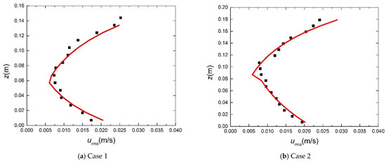
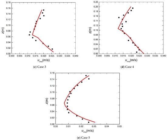
Figure 6. Comparison of the measured and analytical turbulence intensity. Black squares denote the measured data and red lines denote the analytical ones.

To find the difference between analytical and measured data, the error analysis was conducted. An absolute error is defined as the difference between analytical and measured time-averaged velocities. Hence, the average absolute error is calculated as

$$\overline{{\Delta }_a}=\frac{1}{N}{\displaystyle \sum }_1^N\left|{\left(I\right)}_{analytical}-{\left(I\right)}_{measured}\right|$$

(27)

where $N$ is the number of measured points in each measured line for each case, ${\left(I\right)}_{analytical}$ and ${\left(I\right)}_{measured}$ are the analytical and measured values and $I$ represents the variables, i.e., longitudinal velocity, Reynolds stress and turbulence intensity.

The average relative error is defined as

$$\overline{{\Delta }_r}=\frac{1}{N}{\displaystyle \sum }_1^N\left|\frac{{\left(I\right)}_{analytical}-{\left(I\right)}_{measured}}{{\left(I\right)}_{measured}}\right|\times 100\%$$

(28)

As shown in Table 2, the time-averaged longitudinal velocities obtained from the proposed model were reliable within an accuracy of 0.019 m/s in terms of the average absolute error $\overline{{\Delta }_a}$. The average relative error $\overline{{\Delta }_r}$ was 2.86–10.97%. The average absolute error and average relative error of the Reynolds stress were within 0.093 m/s and 13.63%, respectively. The average absolute error and relative error of the turbulence intensity were within 0.0019 m/s and 12.54%, respectively. All values in Table 2 were below 20%, which further confirmed that the proposed analytical model was reliable and feasible to predict the velocity and turbulence structure in the ice-covered flow.

Table 2. Error statistics for the longitudinal velocity, Reynolds stress and turbulence intensity. $\overline{{\Delta }_a}$ is the average absolute error and $\overline{{\Delta }_r}$ is the average relative error.

Cases	Velocity		Reynolds Stress		Turbulence Intensity
	$\overline{{\Delta }_{\mathit{a}}}(\mathbf{m}/\mathbf{s})$	$\overline{{\Delta }_{\mathit{r}}}(\%)$	$\overline{{\Delta }_{\mathit{a}}}(\mathbf{m}/\mathbf{s})$	$\overline{{\Delta }_{\mathit{r}}}(\%)$	$\overline{{\Delta }_{\mathit{a}}}(\mathbf{m}/\mathbf{s})$	$\overline{{\Delta }_{\mathit{r}}}(\%)$
1	0.0065	3.99	0.036	7.01	0.0013	10.52
2	0.0057	3.18	0.038	10.00	0.0011	8.09
3	0.0059	2.86	0.050	9.11	0.0012	8.05
4	0.011	5.25	0.082	8.42	0.0012	6.99
5	0.019	10.97	0.093	13.63	0.0019	12.54

5.2. Discussion

5.2.1. Manning’s Coefficients $n_b$ and $n_i$

Table 3 lists the calculated Manning’s roughness coefficients of the channel bed and ice cover for each case, i.e., $n_b$ and $n_i$. Manning’s roughness coefficient of the channel bed was 0.012–0.015, and its mean value was 0.0138 with the standard deviation of 0.0012, which verified that $n_b$ hardly changed among all studied cases. Manning’s roughness coefficients of the ice cover in all cases were 0.017–0.02, which had small fluctuations and were lightly larger than those of the channel bed. The mean value of $n_i$ was 0.0182 with a standard deviation of 0.0012. For the experimental channel, Manning’s roughness coefficients of the channel bed and ice cover should be considered two specific constants. We took the mean Manning’s roughness coefficient in each layer as the final Manning’s roughness coefficient. Hence, $n_b$ was set to be 0.0138, and $n_i$ was equal to 0.0182.

Table 3. Values of the model parameters to predict the velocity and Reynolds stress.

Cases	${\mathit{n}}_{\mathit{b}}$	${\mathit{n}}_{\mathit{i}}$	${\mathit{m}}_{\mathit{b}}$	${\mathit{m}}_{\mathit{i}}$	${\mathit{h}}_{\mathit{m}}/\mathit{H}$		${\mathit{h}}_{\mathit{\tau }}/\mathit{H}$
					Calculated	Measured	Calculated	Measured
1	0.013	0.018	6.35	4.84	0.43	0.56	0.37	0.35
2	0.012	0.017	7.13	5.31	0.43	0.58	0.43	0.44
3	0.015	0.017	5.41	4.96	0.48	0.42	0.43	0.43
4	0.014	0.02	6.57	4.30	0.40	0.44	0.39	0.44
5	0.015	0.019	5.63	4.59	0.45	0.54	0.39	0.39

5.2.2. Flow Parameters $m_b$ and $m_i$

The values of exponents $m_b$ and $m_i$ in this study are shown in Table 3. All values of $m_b$ were $5.4\le m_b\le 7.1$, and all $m_i$ were $4.3\le m_i\le 5.3$. Teal et al. (1994) [27] estimated $m_b$ and $m_i$ by nonlinear regression for more than measured 2300 vertical velocity profiles, and they found that these two parameters were 1.5–8.5, which includes the theoretical range (see Table 3). For an open channel flow, only exponent $m_b$ is considered and is approximately 6–7, which is unlike the values used here. Hence, both $m_b$ and $m_i$ in the covered flow are affected by the roughness characteristics of both the channel bed and ice cover.

The shape of the vertical profile of the longitudinal velocity is determined by exponents $m_b$ and $m_i$. The ratio of them can be given from Equation (17) as

$$\frac{m_i}{m_b}={\left(\frac{h_i}{h_b}\right)}^{1/6}\frac{n_b}{n_v}$$

(29)

According to Equation (29), the ratio of $m_b$ and $m_i$ is mainly influenced by the roughness coefficients of the channel bed and ice cover. This result is also confirmed by the measured data of Li et al. (2020) [29]. They demonstrate that the vertical distribution of the velocity remains constant with changing water depth and flow rate under the same $m_b$ and $m_i$ or the same ratio of $m_b$ and $m_i$. In the asymmetric flow, the maximum velocity tended to be closer to the smooth boundary with smaller roughness coefficient. In Table 3, the channel bed had a smaller roughness coefficient than the ice cover, which corresponded to the close maximum velocity to the channel bed, which was verified by $h_m<H-h_m$. In general, both open channel flow and symmetry flow can be considered as the special cases of asymmetric flow. For the open channel flow, the exponent $m_i$ tends to infinity. For the symmetry flow, $m_b=m_i$.

5.2.3. Comparison of $h_m$ and $h_{\tau }$

Table 3 presents the locations ($h_m$ and $h_{\tau }$) where the maximum velocity and zero shear stress occur for all cases. These two locations were not consistent and had distinct difference, i.e., calculated $h_m/H>h_{\tau }/H$. The location of zero shear stress is closer to the channel bed than that of maximum velocity [13,29,38]. By contrast, the locations of the maximum velocity and zero shear stress for the symmetry and open channel flows were the same. Specifically, the location of maximum velocity and zero shear stress for the symmetry flows was at the middle water depth, and the location for the open channel flows was at the free water surface.

Considering the locations of the maximum velocity and zero shear stress for cases 1, 3 and 5, when the ratio of $n_i$ to $n_b$ increased, $h_m/H$ decreased, so the location of the maximum velocity approached the channel bed, and the vertical inhomogeneity of the velocity profile was strengthened. Meanwhile, ${\tau }_i/{\tau }_b$ increased with the increase in $n_i/n_b;$ then, $h_{\tau }/H$ decreased, which indicates the location of the zero shear stress gets closer to the channel bed.

5.2.4. Empirical Constants $D_b$, $E_b$, $D_i$ and $E_i$

The empirical constants of turbulence intensity for all cases are listed in Table 4. No remarkable changes of $D_b$ and $D_i$ were observed in any case. The mean $D_b$ was 2.22 with a standard deviation of 0.05, and the mean $D_i$ was 2.16 with a standard deviation of 0.06. Hence, it is reasonable to consider that $D_b=D_i$. The difference between $E_b$ and $E_i$ was not negligible, similar to the results of Li et al. (2020) [29].

Table 4. Parameters to predict the turbulence intensity in each case.

Cases	${\mathit{D}}_{\mathit{b}}$	${\mathit{E}}_{\mathit{b}}$	${\mathit{D}}_{\mathit{i}}$	${\mathit{E}}_{\mathit{i}}$
1	2.22	1.44	2.06	1.82
2	2.21	1.46	2.13	1.87
3	2.22	1.73	2.24	1.50
4	2.15	1.00	2.21	1.83
5	2.31	1.81	2.16	1.51

6. Conclusions

The existence of ice cover dramatically changed the flow velocity and turbulence structure. We here proposed theoretical models to describe the vertical distribution of longitudinal velocity, shear stress and turbulence intensity. By dividing the ice-covered flow into an ice-affected layer and a channel bed-affected layer, a two-power-law function was adopted to predict the vertical profile of velocity. The calculated velocity distribution presents that the maximum velocity occurred near the middle of the water depth close to the channel bed with smooth boundary. Theoretical analysis shows that the shear stress had a linear distribution form in the vertical direction, with the positive values in the lower bed layer and negative values in the upper ice layer. Moreover, the Manning’s roughness coefficient of the ice cover was larger than that of the channel bed. The two exponents $m_b$ and $m_i$ were influenced by the roughness coefficients of the channel bed and ice cover. The location of zero shear stress was not the same as that of maximum velocity and was closer to the smooth fixed boundary than the plane of maximum velocity, namely, $h_m>h_{\tau }$. A comparison of the analytical and experimental velocities, the Reynolds stress and turbulence intensity displays that the theoretical models can provide satisfied predictions of the vertical distribution of these flow characteristics. This study expands our understanding of the effects of ice cover on the hydraulic characteristics in the open channels. However, we still need to do more research to explore the application of the proposed models in other conditions, like compound channels or confluence channels and we will involve comprehensive experiments to reveal detailed flow characteristics, such as vortex structure.

References

- Davar, K.S.; Elhadi, N.A. Management of ice-covered rivers: Problems and perspectives. J. Hydrol. 1981, 51, 245–253. [Google Scholar] [CrossRef]
- Chen, Y.; Wang, Z.; Zhu, D.; Liu, Z. Longitudinal dispersion coefficient in ice-covered rivers. J. Hydraul. Res. 2016, 54, 558–566. [Google Scholar] [CrossRef]
- Chen, G.; Gu, S.; Li, B.; Zhou, M.; Huai, W. Physically based coefficient for streamflow estimation in ice-covered channels. J. Hydrol. 2018, 563, 470–479. [Google Scholar] [CrossRef]
- Knack, I.; Shen, H.-T. Sediment transport in ice-covered channels. Int. J. Sediment Res. 2015, 30, 63–67. [Google Scholar] [CrossRef]
- Lee, M.; Moser, R.D. Direct numerical simulation of turbulent channel flow up to Reτ ≈ 5200. J. Fluid Mech. 2015, 774, 395–415. [Google Scholar] [CrossRef]
- Lotsari, E.; Tarsa, T.; Mri, M.K.; Alho, P.; Kasvi, E. Spatial variation of flow characteristics in a subarctic meandering river in ice-covered and open-channel conditions: A 2d hydrodynamic modelling approach. Earth Surf. Process. Landf. 2019, 44, 1509–1529. [Google Scholar] [CrossRef]
- Turcotte, B.; Morse, B.; Bergeron, N.E.; Roy, A.G. Sediment transport in ice-affected rivers. J. Hydrol. 2011, 409, 561–577. [Google Scholar] [CrossRef]
- Wang, F.; Huai, W.; Liu, M.; Fu, X. Modeling depth-averaged streamwise velocity in straight trapezoidal compound channels with ice cover. J. Hydrol. 2020, 585, 124336. [Google Scholar] [CrossRef]
- Smith, B.T.; Ettema, R. Flow Resistance in Ice-Covered Alluvial Channels. J. Hydraul. Eng. 1997, 123, 592–599. [Google Scholar] [CrossRef]
- Wang, J.; Wu, Y.; Sui, J.; Karney, B. Formation and movement of ice accumulation waves under ice cover—An experimental study. J. Hydrol. Hydromech. 2019, 67, 171–178. [Google Scholar] [CrossRef]
- Namaee, M.R.; Sui, J. Velocity profiles and turbulence intensities around side-by-side bridge piers under ice-covered flow condition. J. Hydrol. Hydromech. 2020, 68, 70–82. [Google Scholar] [CrossRef]
- Hanjalić, K.; Launder, B.E. Fully developed asymmetric flow in a plane channel. J. Fluid Mech. 1972, 51, 301–335. [Google Scholar] [CrossRef]
- Parthasarathy, R.N.; Muste, M. Velocity Measurements in Asymmetric Turbulent Channel Flows. J. Hydraul. Eng. 1994, 120, 1000–1020. [Google Scholar] [CrossRef]
- Tatinclaux, J.; Gogus, M. Asymmetric Plane Flow with Application to Ice Jams. J. Hydraul. Eng. 1983, 109, 1540–1554. [Google Scholar] [CrossRef]
- Lau, Y.L.; Krishnappan, B.G. Sediment Transport Under Ice Cover. J. Hydraul. Eng. 1985, 111, 934–950. [Google Scholar] [CrossRef]
- Muste, M.; Braileanu, F.; Ettema, R. Flow and sediment transport measurements in a simulated ice-covered channel. Water Resour. Res. 2000, 36, 2711–2720. [Google Scholar] [CrossRef]
- Robert, A.; Tran, T. Mean and turbulent flow fields in a simulated ice-covered channel with a gravel bed: Some laboratory observations. Earth Surf. Process. Landforms 2012, 37, 951–956. [Google Scholar] [CrossRef]
- Tao, L. Experimental Study on vertical velocity distribution of water flow under ice sheet. Eng. Constr. 2015, 29, 370–371. [Google Scholar]
- Shen, H.T.; Harden, T.O. The effect of ice cover on vertical transfer in stream channels. J. Am. Water Resour. Assoc. 1978, 14, 1429–1439. [Google Scholar] [CrossRef]
- Lau, Y.L.; Krishnappan, B.G. Ice Cover Effects on Stream Flows and Mixing. J. Hydraul. Div. 1981, 107, 1225–1242. [Google Scholar] [CrossRef]
- Chen, G.; Gu, S.; Huai, W.; Zhang, Y. Boundary Shear Stress in Rectangular Ice-Covered Channels. J. Hydraul. Eng. 2015, 141, 06015005. [Google Scholar] [CrossRef]
- Attar, S.; Li, S. Data-fitted velocity profiles for ice-covered rivers. Can. J. Civ. Eng. 2012, 39, 334–338. [Google Scholar] [CrossRef]
- Sui, J.; Wang, J.; Yun, H.E.; Krol, F. Velocity profiles and incipient motion of frazil particles under ice cover. Int. J. Sediment Res. 2010, 25, 39–51. [Google Scholar] [CrossRef]
- Larsen, P.A. Head losses caused by an ice cover on open channels. J. Boston Soc. Civ. Eng. 1969, 56, 45–67. [Google Scholar]
- Sayre, W.W.; Song, G.B. Effects of Ice Covers on Alluvial Channel Flow and Sediment Transport Processes. IIHR Report No. 218, University of Lowa. Available online: https://apps.dtic.mil/dtic/tr/fulltext/u2/a066991.pdf (accessed on 16 April 2021).
- Uzuner, M.S. The composite roughness of ice covered streams. J. Hydraul. Res. 1975, 13, 79–102. [Google Scholar] [CrossRef]
- Teal, M.J.; Ettema, R.; Walker, J.F. Estimation of Mean Flow Velocity in Ice-Covered Channels. J. Hydraul. Eng. 1994, 120, 1385–1400. [Google Scholar] [CrossRef]
- Tsai, W.; Ettema, R. Modified Eddy Viscosity Model in Fully Developed Asymmetric Channel Flows. J. Eng. Mech. 1994, 120, 720–732. [Google Scholar] [CrossRef]
- Li, Q.; Zeng, Y.-H.; Bai, Y. Mean flow and turbulence structure of open channel flow with suspended vegetation. J. Hydrodyn. 2020, 32, 314–325. [Google Scholar] [CrossRef]
- Zhang, J.; Lei, J.; Huai, W.; Nepf, H. Turbulence and Particle Deposition Under Steady Flow Along a Submerged Seagrass Meadow. J. Geophys. Res. Oceans 2020, 125, 2019–015985. [Google Scholar] [CrossRef]
- Rowiński, P.M.; Kubrak, J. A mixing-length model for predicting vertical velocity distribution in flows through emergent vegetation. Hydrol. Sci. J. 2002, 47, 893–904. [Google Scholar] [CrossRef]
- Nezu, I.; Rodi, W. Open-channel Flow Measurements with a Laser Doppler Anemometer. J. Hydraul. Eng. 1986, 112, 335–355. [Google Scholar] [CrossRef]
- Zhong, Y.; Huai, W.; Chen, G. Analytical Model for Lateral Depth-Averaged Velocity Distributions in Rectangular Ice-Covered Channels. J. Hydraul. Eng. 2019, 145, 04018080. [Google Scholar] [CrossRef]
- Huai, W.-X.; Xu, Z.-G.; Yang, Z.-H.; Zeng, Y.-H. Two dimensional analytical solution for a partially vegetated compound channel flow. Appl. Math. Mech. 2008, 29, 1077–1084. [Google Scholar] [CrossRef]
- Bonakdari, H.; Larrarte, F.; Lassabatere, L.; Joannis, C. Turbulent velocity profile in fully-developed open channel flows. Environ. Fluid Mech. 2008, 8, 1–17. [Google Scholar] [CrossRef]
- Zare, S.G.A.; Moore, S.A.; Rennie, C.D.; Seidou, O.; Ahmari, H.; Malenchak, J. Estimation of composite hydraulic resistance in ice-covered alluvial streams. Water Resour. Res. 2016, 52, 1306–1327. [Google Scholar] [CrossRef]
- Han, L.; Zeng, Y.; Chen, L.; Li, M. Modeling streamwise velocity and boundary shear stress of vegetation-covered flow. Ecol. Indic. 2018, 92, 379–387. [Google Scholar] [CrossRef]
- Papanicolaou, A.N.; Elhakeem, M.; Hilldale, R. Secondary current effects on cohesive river bank erosion. Water Resour. Res. 2007, 43, 497–507. [Google Scholar] [CrossRef]
Publisher’s Note: MDPI stays neutral with regard to jurisdictional claims in published maps and institutional affiliations. |
© 2021 by the authors. Licensee MDPI, Basel, Switzerland. This article is an open access article distributed under the terms and conditions of the Creative Commons Attribution (CC BY) license (https://creativecommons.org/licenses/by/4.0/).